A Surface Family with a Mutual Geodesic Curve in Galilean 3-Space ${\mathbb{G}}_3$

Abstract

This article gives an approach for establishing a surface family with a mutual geodesic curve in Galilean 3-space ${\mathbb{G}}_3$. Given a smooth space curve, we derive the sufficient and necessary condition for the given curve to be geodesic on it. Furthermore, we resolve the conditions when the surface is a ruled surface. Consequently, its ability to develop with the mutual geodesic of the elements of the surface family is researched. Meanwhile, we explain this approach by submitting considerable examples.

1. Introduction

A geodesic curve is one of the most significant considerable curves on a surface. Through a geodesic curve, the normal vector to the geodesic is identical with the surface normal vector. In other words, the normal vector of a curve is meantime parallel to the normal of the surface [1,2]. The geodesic also plays a role in the relativistic characterization of gravity. Einstein’s idea of equalness says that the geodesic appears in the trajectory of a freely falling particle in a given space (freely landing in this status means only movable down the effect of gravity, with no other forces implicated). The geodesic idea states that the free trajectory is the geodesics of space. It plays a fully significant role in a geometric-relativity theory, since it means that the basic equation of dynamics is fully specified by the geometry of space, and subsequently does not need to be set as an independent equation. Furthermore, in such a theory, the behavior is identified (up to a constant) by the essential length invariant, so that the stable behavior principal and the geodesic principle become identical [3,4]. The notion of the geodesic also find its position in distinct industrial implementations, such as cutting and painting track, tent manufacturing, and textile manufacturing [5,6,7,8,9,10,11,12]. The major objective of these studies is determining how these surfaces can be built with this curve as a geodesic curve.

Galilean space is the limit case of a semi-Euclidean space for which the isotropic cone degenerates to a plane. It is explained as a Cayley–Klein geometry of the product space which acts as a significant part in physics. The major dissimilarity of Galilean geometry is its special simplicity, as it authorizes the scholar to research it in detail without losing a large package of time and intellectual energy. Set differently, the clarity of Galilean geometry constructs its comprehensive evolution as an easy issue, and the comprehensive expansion of a novel geometric regulation is a prerequisite for efficiently comparing it with Euclidean geometry. Furthermore, comprehensive evolution can possibly give the scholar the psychological emphasis of the coherence of the inspected structure [3]. In the $3\mathbb{D}$ (three-dimensional) Galilean space ${\mathbb{G}}_3$, the applicable action on surfaces with a geodesic curve is scarce. It is a serious and fascinating trouble in functional implementations. In [13], Abdel-Aziz, and Khalifa considered the location vector of a random curve in the Galilean 3-space ${\mathbb{G}}_3$. Furthermore, they gave several conditions on the curvatures of this random curve to investigate the specific curves and their Smarandache curves. Yuzbas and Bektas investigated the parametrization for a set of surfaces over a given geodesic curve. They derived necessary and sufficient conditions for this curve to be an iso-geodesic curve on the parametric surfaces [14]. The problem of constructing a hypersurface family with a mutual geodesic curve in the 4D Galilean space ${\mathbb{G}}_4$ has been addressed in [15,16,17]. Therefore, designing a surface from a given curve in Galilean 3-space ${\mathbb{G}}_3$ is attractive.

In this paper, we adopt a different means of designing surfaces—all share a given geodesic curve as an iso-parametric curve. Given a smooth space curve, we first answer the question regarding the sufficient and necessary condition for the given curve to be geodesic. In the procedure of inference, the sufficient and necessary conditions when the resulting surface is a ruled surface are also analyzed. Meanwhile, various representative curves are chosen to confirm this approach. The paramount point to note here is the method we utilized (compared with [14]).

2. Basic Concepts

The Galilean 3-space ${\mathbb{G}}_3$ is a Cayley–Klein geometry furnished with the projective metric of signature $(0,0,+,+)$ [18,19]. The absolute figure of the Galilean space depending on the organized triple {$\omega$, f, I}, where $\omega$ is the (absolute) plane in the real 3-dimensional projective space ${\mathbb{P}}^3$($\mathbb{R}$), f is the line (absolute line) in $\omega$, and I the stationary elliptic involution of points of f. The homogeneous coordinates in ${\mathbb{G}}_3$ are presented in such a manner that the absolute plane $\omega$ is given by $x_0=0$, the absolute line f by $x_0=x_1=0$, and the elliptic involution is given by $(0:0:x_2:x_3)\to (0:0:x_3:-x_2)$. A plane is named Euclidean if it includes f, otherwise it is named isotropic, that is, the planes x=const are Euclidean, and so is the plane $\omega$. Other planes are isotropic. In other words, an isotropic plane does not involve any isotropic orientation.

For any $\alpha =\left({\alpha }_1,{\alpha }_2,{\alpha }_3\right)$, and $\beta$$=\left({\beta }_1,{\beta }_2,{\beta }_3\right)\in {\mathbb{G}}_3$, their scalar product is

$$<\mathit{\alpha },\mathit{\beta }>=\left\{\begin{array}{c}{\alpha }_1{\beta }_1,\mathrm{if}{\alpha }_1\ne 0\vee {\beta }_1\ne 0\hfill \\ {\alpha }_2{\beta }_2+{\alpha }_3{\beta }_3,\mathrm{if}{\alpha }_1=0\wedge {\beta }_1=0,\hfill \end{array}\right.$$

(1)

and their vector product is

$$\mathit{\alpha }\times \mathit{\beta }=\left\{\begin{array}{c}\left|\begin{array}{ccc}\mathbf{0}\hfill & {\mathit{e}}_2\hfill & {\mathit{e}}_3\hfill \\ {\alpha }_1\hfill & {\alpha }_2\hfill & {\alpha }_3\hfill \\ {\beta }_1\hfill & {\beta }_2\hfill & {\beta }_3\hfill \end{array}\right|,\mathrm{if}{\alpha }_1\ne 0\vee {\beta }_1\ne 0,\\ \left|\begin{array}{ccc}{\mathit{e}}_1\hfill & {\mathit{e}}_2\hfill & {\mathit{e}}_3\hfill \\ 0\hfill & {\alpha }_2\hfill & {\alpha }_3\hfill \\ 0\hfill & {\beta }_2\hfill & {\beta }_3\hfill \end{array}\right|,\mathrm{if}{\alpha }_1=0\wedge {\beta }_1=0.\end{array}\right.$$

(2)

where ${\mathit{e}}_1=(1,0,0)$, ${\mathit{e}}_2=(0,1,0)$ and ${\mathit{e}}_3=(0,0,1)$ are the standard basis vectors in ${\mathbb{G}}_3$.

A curve $\mathit{\phi }\left(u\right)=\left({\phi }_1\left(u\right),{\phi }_2\left(u\right),{\phi }_3\left(u\right)\right);u\in I\subseteq \mathbb{R}$ is called an allowable curve if it has no inflection points, that is, $\stackrel{.}{\mathit{\phi }}\times \stackrel{..}{\mathit{\phi }}\ne \mathbf{0}$ and no isotropic tangents $\stackrel{.}{{\phi }_1}\ne 0$. An allowable curve is a similar to a smooth curve in Euclidean space. For an allowable curve $\mathit{\phi }$: $I\subseteq \mathbb{R}\to {\mathbb{G}}_3$ represented by the Galilean invariant arc-length s, we have:

$$\mathit{\phi }\left(s\right)=\left(s,{\phi }_2\left(s\right),{\phi }_3\left(s\right)\right).$$

The curvature $\kappa \left(s\right)$ and torsion $\tau \left(s\right)$ of the curve $\phi$$\left(s\right)$ are

$$\begin{array}{ccc}\hfill \kappa \left(s\right)& =& ∥{\mathit{\phi }}^{{}^{″}}\left(s\right)∥=\sqrt{{\left({\phi }_2^{{}^{″}}\left(s\right)\right)}^2+{\left({\phi }_3^{{}^{″}}\left(s\right)\right)}^2},\hfill \\ \hfill \tau \left(s\right)& =& \frac{1}{{\kappa }^2\left(s\right)}det\left({\mathit{\phi }}^{{}^{\prime }},{\mathit{\phi }}^{{}^{{}^{″}}},{\mathit{\phi }}^{{}^{{}^{{}^{‴}}}}\right).\hfill \end{array}$$

(3)

Note that an allowable curve has $\kappa \left(s\right)\ne 0$. The related Serret–Frenet vectors are [18,19]:

$$\begin{array}{ccc}\hfill {\mathit{\upsilon }}_1\left(s\right)& =& {\mathit{\phi }}^{{}^{\prime }}\left(s\right)=\left(1,{\phi }_2^{{}^{\prime }}\left(s\right),{\phi }_3^{{}^{\prime }}\left(s\right)\right),\hfill \\ \hfill {\mathit{\upsilon }}_2\left(s\right)& =& \frac{1}{\kappa \left(s\right)}{\mathit{\phi }}^{{}^{\prime }}\left(s\right)=\frac{1}{\kappa \left(s\right)}\left(0,{\phi }_2^{{}^{″}}\left(s\right),{\phi }_3^{{}^{″}}\left(s\right)\right),\hfill \\ \hfill {\mathit{\upsilon }}_3\left(s\right)& =& \frac{1}{\tau \left(s\right)}\left(0,{\left(\frac{1}{\kappa \left(s\right)}{\phi }_2^{{}^{″}}\left(s\right)\right)}^{{}^{\prime }},{\left(\frac{1}{\kappa \left(s\right)}{\phi }_3^{{}^{″}}\left(s\right)\right)}^{{}^{\prime }}\right),\hfill \end{array}$$

(4)

where ${\mathit{\upsilon }}_1\left(s\right)$, ${\mathit{\upsilon }}_2\left(s\right)$, and ${\mathit{\upsilon }}_3\left(s\right)$, respectively, are the tangent, principal normal, and binormal vectors. For every point of $\mathit{\phi }\left(s\right)$, the Serret–Frenet formula reads:

$$\left(\begin{array}{c}{\mathit{\upsilon }}_1^{{}^{\prime }}\hfill \\ {\mathit{\upsilon }}_2^{{}^{\prime }}\hfill \\ {\mathit{\upsilon }}_3^{{}^{\prime }}\hfill \end{array}\right)=\left(\begin{array}{ccc}0\hfill & \kappa \left(s\right)\hfill & 0\hfill \\ 0\hfill & 0\hfill & \tau \left(s\right)\hfill \\ 0\hfill & -\tau \left(s\right)\hfill & 0\hfill \end{array}\right)\left(\begin{array}{c}{\mathit{\upsilon }}_1\hfill \\ {\mathit{\upsilon }}_2\hfill \\ {\mathit{\upsilon }}_3\hfill \end{array}\right).$$

(5)

The planes which match to the subspaces Sp{${\mathit{\upsilon }}_1,$${\mathit{\upsilon }}_2$}, Sp{${\mathit{\upsilon }}_2$, ${\mathit{\upsilon }}_3$}, and Sp{${\mathit{\upsilon }}_3$, ${\mathit{\upsilon }}_1$}, respectively, are named the osculating plane, normal plane, and rectifying plane. We indicate a surface M in ${\mathbb{G}}_3$ by

$$M:\mathit{y}(s,t)=\left(y_1\left(s,t\right),y_2\left(s,t\right),y_3\left(s,t\right)\right),(s,t)\in D\subseteq {\mathbb{R}}^2.$$

(6)

If ${\mathit{y}}_j(s,t)=\frac{\partial \mathit{y}}{\partial j}$, the isotropic surface normal is

$$\mathit{\xi }(s,t)={\mathit{y}}_s\wedge {\mathit{y}}_t,$$

(7)

which is orthogonal to each of the vectors ${\mathit{y}}_s$, and ${\mathit{y}}_t$.

Definition 1

([1,2]). A curve on a surface is a geodesic if and only if the normal vector of the curve is everywhere parallel to surface normal.

A curve $\mathit{\alpha }\left(s\right)$ on a surface $\mathit{y}(s,t)$ is an isoparametric curve if it has a constant s or t-parameter value. In other words, there exists a parameter $t_0$ such that $\mathit{\alpha }\left(s\right)=\mathit{y}(s,t_0)$ or $\mathit{\alpha }\left(t\right)=\mathit{y}(s_0,t)$. Given a parametric curve $\mathit{\alpha }\left(s\right)$, we call it an iso-geodesic of the surface $\mathit{y}(s,t)$ if it is both a geodesic and a parameter curve on $\mathit{y}(s,t)$.

3. Surfaces with a Mutual Geodesic Curve in ${\mathbb{G}}_3$

This section prepares a new approach for constructing a surface family from a given geodesic curve in ${\mathbb{G}}_3$. To do this, we take into account $\mathit{\beta }\left(s\right)$, $0\le s\le L$, such that the rectifying plane $Sp\{{\mathit{\upsilon }}_1$, ${\mathit{\upsilon }}_3$} is congruous with surface family tangent plane. Then,

$$M:\mathit{y}(s,t)=\mathit{\phi }\left(s\right)+u(s,t){\mathit{\upsilon }}_1\left(s\right)+v(s,t){\mathit{\upsilon }}_3\left(s\right);0\le t\le T,$$

(8)

where $u(s,t),$ and $v(s,t)$ are all $C^1$ functions. If the variable t is seen as the time, then $u(s,t),$ and $v(s,t)$ can be viewed as the oriented marching distances of a point unit in time t in the orientation ${\mathit{\upsilon }}_1$ and ${\mathit{\upsilon }}_3$, respectively; and $\mathit{\phi }\left(s\right)$ is seen as the initial location of this point.

Then, we can have

$$\left.\begin{array}{c}{\mathit{y}}_s(s,t)=(1+u_s){\mathit{\upsilon }}_1+(u\kappa -\tau v){\mathit{\upsilon }}_2+\tau v_s{\mathit{\upsilon }}_3,\hfill \\ {\mathit{y}}_t(s,t)=u_t\mathit{t}+v_t{\mathit{\upsilon }}_3,\hfill \end{array}\right\}$$

(9)

and

$$\mathit{\xi }(s,t):={\mathit{y}}_s\times {\mathit{y}}_t=\left[-(1+u_s)v_t+v_s{u}_t\right]{\mathit{\upsilon }}_2-\left(u\kappa -\tau v\right)u_t{\mathit{\upsilon }}_3.$$

(10)

Since $\mathit{\phi }\left(s\right)$ is an iso-parametric on the surface, there exists a value $t=t_0\in [0,T]$ such that $\mathit{y}(s,t_0)=\mathit{\phi }\left(s\right)$; that is,

$$u(s,t_0)=v(s,t_0)=0,u_s(s,t_0)=v_s(s,t_0)=0.$$

(11)

Thus, when $t=t_0$—i.e., over $\mathit{\phi }\left(s\right)$, we have

$$\mathit{\xi }(s,t_0)=-v_t(s,t_0){\mathit{\upsilon }}_2\left(s\right).$$

(12)

Congruous of the principal normal ${\mathit{\upsilon }}_2\left(s\right)$ with the surface, the normal $\mathit{\xi }$ recognizes $\mathit{\phi }\left(s\right)$ as a geodesic curve. Hence, from Equations (11) and (12), we have:

Theorem 1.

The curve $\mathit{\phi }:I\subset \mathbb{R}\to {\mathbb{G}}_3$ is an iso-geodesic (geodesic for short) on the surface M if and only if the following conditions are satisfied

$$\left.\begin{array}{c}u(s,t_0)=v(s,t_0)=u_s(s,t_0)=v_s(s,t_0)=0,\hfill \\ \\ v_t(s,t_0)\ne 0,0\le t_0\le T,0\le s\le L.\hfill \end{array}\right\}$$

(13)

For the above conditions in Theorem 1, $u(s,t),$ and $v(s,t)$ can be written as:

$$\begin{array}{c}u(s,t)=l\left(s\right)U\left(t\right),\\ v(s,t)=m\left(s\right)V\left(t\right).\end{array}$$

(14)

Here, the $l\left(s\right)$, $m\left(s\right),U\left(t\right)$, and $v\left(t\right)$ are $C^1$ functions do not identically vanish. Hence, from Theorem 1, we gain:

Corollary 1.

If $u(s,t)$ and $v(s,t)$ are the same as they are in Equation (14), then the sufficient and necessary condition for $\mathit{\phi }\left(s\right)$ to be a geodesic on M is

$$\left.\begin{array}{c}U\left(t_0\right)=V\left(t_0\right)=0,l\left(s\right)=const.,m\left(s\right)=const.\ne 0,\hfill \\ \frac{dV\left(t_0\right)}{dt}=const.\ne 0,0\le t_0\le T,0\le s\le L.\hfill \end{array}\right\}$$

(15)

It is worth noting that, to gain a surface family, with a mutual geodesic curve, we can first have Equations (15), and then employ them to Equation (8) to have the family. For suitability in the performance, $u(s,t)$ and $v(s,t)$ can be chosen in two special forms:

(1) If

$$\left\{\begin{array}{c}u(s,t)=\underset{k=1}{\stackrel{p}{\mathrm{\Sigma }}}{x}_{1k}l{\left(s\right)}^{k}U{\left(t\right)}^k,\\ v(s,t)=\underset{k=1}{\stackrel{p}{\mathrm{\Sigma }}}{x}_{2k}m{\left(s\right)}^{k}V{\left(t\right)}^k,\end{array}\right.$$

(16)

then, we can completely express the sufficient condition for which the curve $\mathit{\phi }\left(s\right)$ is a geodesic curve on the surface $\mathit{y}(s,t)$ as:

$$\left\{\begin{array}{c}U\left(t_0\right)=V\left(t_0\right)=0,\\ a_{21}\ne 0,m\left(s\right)\ne 0,\mathrm{and}\frac{dV\left(t_0\right)}{dt}\ne 0,\end{array}\right.$$

(17)

where $l\left(s\right),$ $m\left(s\right),$ $U\left(t\right),$ and $V\left(t\right)$ are $C^1$ functions, $a_{ij}\in \mathbb{R}$$(i=1,2;j=1,2,...,p)$ and $l\left(s\right)$, and $m\left(s\right)$ do not identically vanish.

(2) If we choose

$$\left\{\begin{array}{c}u(s,t)=\underset{k=1}{\stackrel{p}{f(\mathrm{\Sigma }}}{x}_{1k}{l}^k\left(s\right)U^k\left(t\right)),\\ v(s,t)=g\left(\underset{k=1}{\stackrel{p}{\mathrm{\Sigma }}}{x}_{2k}{m}^k\left(s\right)V^k\left(t\right)\right),\end{array}\right.$$

(18)

then we can rewrite Equation (15), for which the curve $\mathit{\phi }\left(s\right)$ is a geodesic curve on the surface $\mathit{y}(s,t),$ as:

$$\left\{\begin{array}{c}U\left(t_0\right)=V\left(t_0\right)=v\left(t_0\right)=f\left(0\right)=g\left(0\right)=0,\\ x_{21}\ne 0,\frac{dV\left(t_0\right)}{dt}=const\ne 0,m\left(s\right)\ne 0,g^{{}^{\prime }}\left(0\right)\ne 0,\end{array}\right.$$

(19)

where $l\left(s\right),$ $m\left(s\right),$ $U\left(t\right),$ $V\left(t\right)$, f, and g are $C^1$ functions. Since there is no restriction attached to the given curve in Equations (15), (17), or (19), the surface family with $\mathit{\beta }\left(s\right)$ as the mutual geodesic, can constantly be established by choosing suitable marching-scale functions. Clearly, Equations (13), (15), (17) and (19) are more convenient and elegant for implementations than those reported [14].

3.1. Examples

The last discussions are explained by the following examples.

Example 1.

Let

$$\mathit{\phi }\left(s\right)=(s,sins,coss),0\le s\le 2\pi .$$

Then,

$$\begin{array}{ccc}\hfill {\mathit{\phi }}^{{}^{\prime }}\left(s\right)& =& (1,coss,-sins),\hfill \\ \hfill {\mathit{\phi }}^{{}^{″}}\left(s\right)& =& (0,-sins,-coss),\hfill \\ \hfill {\mathit{\phi }}^{{}^{{}^{‴}}}\left(s\right)& =& (0,-coss,sins),\hfill \end{array}$$

Using Equations (3) and (4) to gain $\kappa \left(s\right)=1,\tau \left(s\right)=1$, and

$$\begin{array}{ccc}\hfill {\mathit{\upsilon }}_1\left(s\right)& =& (1,coss,-sins),\hfill \\ \hfill {\mathit{\upsilon }}_2\left(s\right)& =& (0,-sins,-coss),\hfill \\ \hfill {\mathit{\upsilon }}_3\left(s\right)& =& (0,coss,-sins).\hfill \end{array}$$

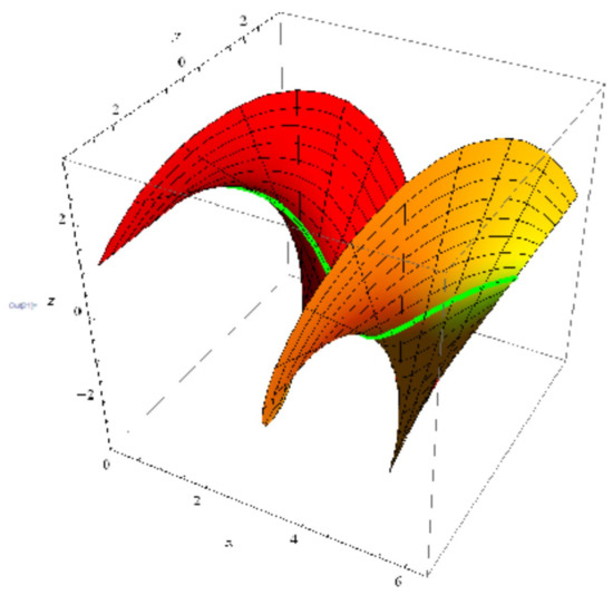
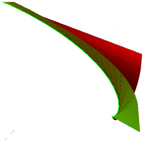
(1) If $u(s,t)=0$, $v(s,t)=-t$, where $t_0=0$, and $-1\le t\le 1$, then Equation (15) is satisfied. Thus, we have a surface with a mutual geodesic curve $\mathit{\phi }\left(s\right)$ as (Figure 1):

$$M:\mathit{y}(s,t)=\left(s,sins-tcoss,coss+tsins\right).$$

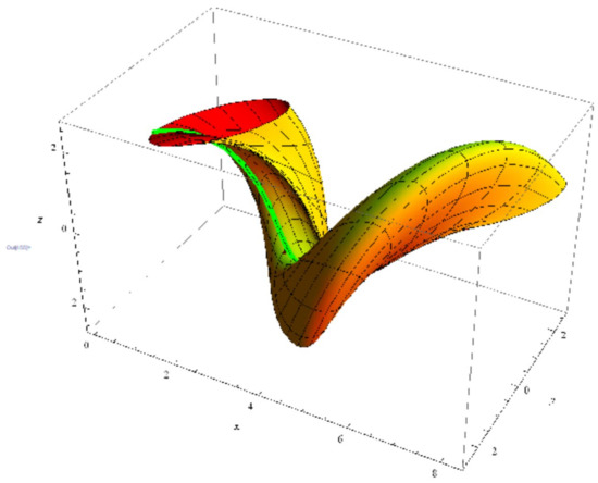
(2) By taking $u(s,t)=1-cott$, $v(s,t)=sint$, $t_0=0$, and $-0.5\le t\le 0.5$, then Equation (19) is satisfied. Then, a member of this family is acquired by (Figure 2):

$$M:\mathit{y}(s,t)=\left(\begin{array}{c}s+1-cott\\ sins+\left(sint+1-cott\right)coss\\ coss-\left(sint+1-cot\left(t\right)\right)sins\end{array}\right).$$

Figure 1. A surface with $\mathit{\phi }$ as a geodesic curve.

Figure 2. A surface with $\mathit{\phi }$ as a geodesic curve.

Example 2.

Let

$$\mathit{\phi }\left(s\right)=(s,1+sins,sins),0\le s\le 2\pi .$$

Similarly, we apply$\phi$${}^{{}^{\prime }}$,$\phi$${}^{{}^{″}}$,$\phi$${}^{{}^{{}^{‴}}}$ to have $\kappa \left(s\right)=\sqrt{2}sins,$$\tau \left(s\right)=0$, and

$$\begin{array}{ccc}\hfill {\mathit{\upsilon }}_1\left(s\right)& =& (1,coss,coss),\hfill \\ \hfill {\mathit{\upsilon }}_2\left(s\right)& =& (0,-\frac{1}{\sqrt{2}},-\frac{1}{\sqrt{2}}),\hfill \\ \hfill {\mathit{\upsilon }}_3\left(s\right)& =& (0,\frac{1}{\sqrt{2}},-\frac{1}{\sqrt{2}}).\hfill \end{array}$$

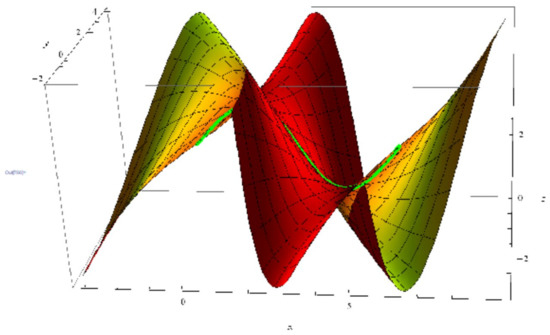
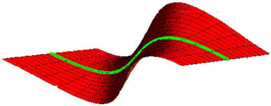
(1) By taking $u(s,t)=t$, $v(s,t)=sint$, $t_0=0$, and $-\pi \le t\le \pi$, then Equation (17) is satisfied. Then, a member of this family is gained by (Figure 3):

$$M:\mathit{y}(s,t)=\left(s+t,1+sins+tcoss+\frac{1}{\sqrt{2}}sint,sins+tcoss-\frac{1}{\sqrt{2}}sint\right).$$

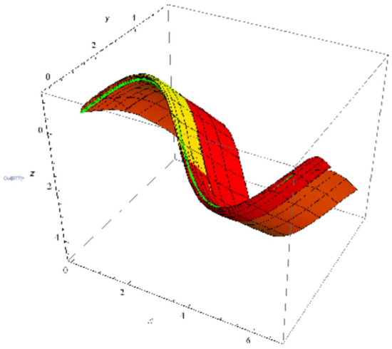
(2) If

$$\left.\begin{array}{c}u(s,t)=\underset{i=1}{\stackrel{2}{\mathrm{\Sigma }}}{cos}^i\left(s\right)\left(1-{cos}^i\left(t\right)\right),\hfill \\ v(s,t)=\underset{i=1}{\stackrel{2}{\mathrm{\Sigma }}}{cosh}^i\left(s\right){sinh}^i\left(t\right),\hfill \end{array}\right\}$$

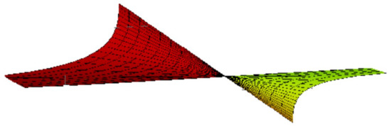
at $t_0=0$ such that Equations (17) are satisfied. Hence, a member of this family is (Figure 4):

$$\mathit{y}(s,t)=\left(\begin{array}{c}s+\underset{i=1}{\stackrel{2}{\mathrm{\Sigma }}}{cos}^i\left(s\right)\left(1-{cos}^i\left(t\right)\right)\\ 1+sins+coss\underset{i=1}{\stackrel{2}{\mathrm{\Sigma }}}{cos}^i\left(s\right)\left(1-{cos}^i\left(t\right)\right)+\frac{1}{\sqrt{2}}\underset{i=1}{\stackrel{2}{\mathrm{\Sigma }}}{cosh}^i\left(s\right){sinh}^i\left(t\right)\\ coss+coss\underset{i=1}{\stackrel{2}{\mathrm{\Sigma }}}{cos}^i\left(s\right)\left(1-{cos}^i\left(t\right)\right)-\frac{1}{\sqrt{2}}\underset{i=1}{\stackrel{2}{\mathrm{\Sigma }}}{cosh}^i\left(s\right){sinh}^i\left(t\right)\end{array}\right),$$

where $0\le s\le 2\pi$ and $-0.003\le t\le 0.003$.

Figure 3. A surface with $\mathit{\phi }$ as a geodesic curve.

Figure 4. A surface with $\mathit{\beta }$ as a geodesic curve.

Noticeably, we could carry on with this series of surfaces, by taking other combinations of special curve obtained to date, or with a greater number of curves to interpolate.

3.2. Ruled Surfaces with a Mutual Geodesic Curve

A ruled surface is realized by one-parameter set of straight lines movable on a curve. The curve is named base (directrix) and the straight line is named ruling. In this subsection, we will examine the structure of the ruled surface with a base curve as a geodesic.

Let $\mathit{y}(s,t)$ be a ruled surface with the base curve $\phi$$\left(s\right)$, and $\phi$$\left(s\right)$ is also an iso-parametric curve of $\mathit{y}(s,t)$, then there exists $t_0$ such that $\mathit{y}(s,t_0)=$$\phi$$\left(s\right)$. Thus, the surface can be acquired as

$$M:\mathit{y}(s,t)-\mathit{y}(s,t_0)=(t-t_0)\mathit{g}\left(s\right),0\le s\le L,\mathrm{with}t,t_0\in [0,T],$$

where $\mathit{y}(s,t_0)=$$\phi$$\left(s\right)$, and $\mathit{g}\left(s\right)$ defines the orientation of the rulings. Considering Equation (8), we obtain

$$(t-t_0)\mathit{g}\left(s\right)=u(s,t){\mathit{\upsilon }}_1\left(s\right)+v(s,t){\mathit{\upsilon }}_3\left(s\right),0\le s\le L,\mathrm{with}t,t_0\in [0,T],$$

(20)

which is a system of two equations with two unknown functions $u(s,t)$, and $v(s,t)$. To resolve $u(s,t)$ and $v(s,t)$, we have

$$\begin{array}{c}u(s,t)=(t-t_0)<\mathit{g}\left(s\right),{\mathit{\upsilon }}_1\left(s\right)>=det(\mathit{g}\left(s\right),{\mathit{\upsilon }}_2\left(s\right),{\mathit{\upsilon }}_3\left(s\right))\\ v(s,t)=(t-t_0)<\mathit{g}\left(s\right),{\mathit{\upsilon }}_3\left(s\right)>=det(\mathit{g}\left(s\right),{\mathit{\upsilon }}_1\left(s\right),{\mathit{\upsilon }}_2\left(s\right)),\end{array}$$

(21)

which are totally the sufficient and necessary conditions for $\mathit{y}(s,t)$ to be a ruled surface with a base curve $\mathit{\phi }\left(s\right)$.

Next, we aimed to examine whether $\mathit{\phi }\left(s\right)$ is also geodesic on $\mathit{y}(s,t)$ by employing the conditions given in Theorem 1. It is obvious that, in this case, we have

$$\begin{array}{c}det(\mathit{g}\left(s\right),{\mathit{\upsilon }}_2\left(s\right),{\mathit{\upsilon }}_3\left(s\right))=0,\\ det(\mathit{g}\left(s\right),{\mathit{\upsilon }}_1\left(s\right),{\mathit{\upsilon }}_2\left(s\right))\ne 0.\end{array}$$

(22)

Thus, at all points on $\mathit{\phi }\left(s\right)$, the ruling $\mathit{g}\left(s\right)\in Sp\{{\mathit{\upsilon }}_1\left(s\right)$,${\mathit{\upsilon }}_3\left(s\right)\}$. Furthermore, the ruling $\mathit{g}\left(s\right)$ and the vector $\mathit{t}\left(s\right)$ should not be parallel. Thus,

$$\mathit{g}\left(s\right)=\alpha \left(s\right){\mathit{\upsilon }}_1\left(s\right)+\gamma \left(s\right){\mathit{\upsilon }}_3\left(s\right),0\le s\le L,$$

(23)

for functions $\alpha \left(s\right)$ and $\gamma \left(s\right)\ne 0$. By replacing it into the Equations (21),we obtain

$$\alpha \left(s\right)t=u(s,t),\gamma \left(s\right)t=v(s,t),0\le s\le L.$$

(24)

Hence, the ruled surface family with the mutual geodesic base $\phi$$\left(s\right)$ can be acquired as

$$M:\mathit{y}(s,t)=\mathit{\phi }\left(s\right)+t(\alpha \left(s\right){\mathit{\upsilon }}_1\left(s\right)+\gamma \left(s\right){\mathit{\upsilon }}_3\left(s\right)),0\le s\le L,0\le t\le T.$$

(25)

$\alpha \left(s\right)$, and $\gamma \left(s\right)\ne 0$ can control the form of the surface family. It is clear that

$$\mathit{\xi }(s,t)=t\gamma \left(\gamma \tau -\kappa {\alpha }^{{}^{\prime }}\right){\mathit{\upsilon }}_1+\left[\alpha {\gamma }^{{}^{\prime }}-(1+t{\alpha }^{{}^{\prime }})\gamma \right]{\mathit{\upsilon }}_2+\left(\gamma \tau -\alpha \kappa \right){\mathit{\upsilon }}_3.$$

(26)

and thus, when $t=0$, that is, along $\phi$$\left(s\right)$, the surface normal is

$$\mathit{\xi }(s,0)=-\gamma \left(s\right){\mathit{\upsilon }}_2.$$

(27)

Theorem 2.

The sufficient and necessary condition for M to be a ruled surface with$\phi$$\left(s\right)$ as a geodesic is that there exists a parameter $t=t_0\in [0,T]$, as well as the functions $\alpha \left(s\right)$ and $\gamma \left(s\right)\ne 0$, so that M can be determined by Equation (25).

Notice that, in this family, there exist two geodesic curves crossing during each point on $\phi$$\left(s\right)$: one is $\phi$$\left(s\right)$ itself and the other is a straight line in the orientation $\mathit{g}\left(s\right)$ as in Equation (23). All the elements of the iso-geodesic ruled surfaces is specified by two functions $\alpha \left(s\right)$, and $\gamma \left(s\right)\ne 0$, that is, by the orientation vector function $\mathit{g}\left(s\right)$. In Example 1 for $\alpha \left(s\right)=\gamma \left(s\right)=s$, the ruled surface is shown in Figure 5. Figure 6 shows the surface with $\alpha \left(s\right)=0$ and $\gamma \left(s\right)=1$.

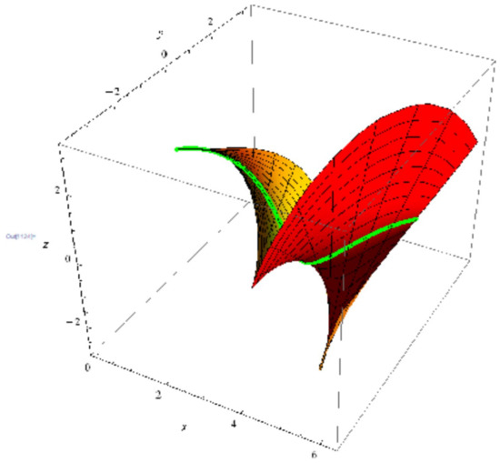
Figure 5. Ruled surface with $\alpha \left(s\right)=\gamma \left(s\right)=s$.

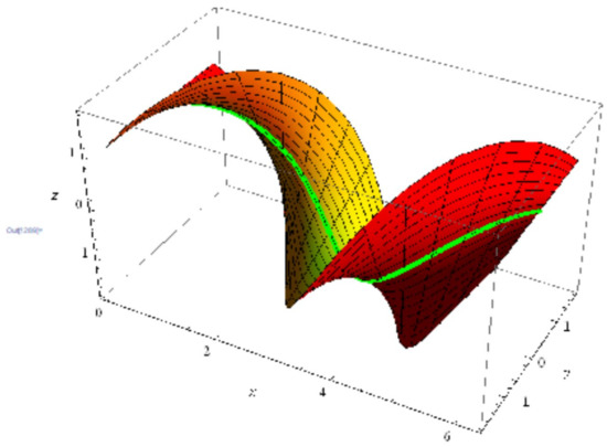
Figure 6. Ruled surface with $\alpha \left(s\right)=0$ and $\gamma \left(s\right)=1$.

Developable Surfaces

Developable surfaces are simple and mutual surfaces in surface modeling. There are three types of developable surfaces, the given curve can be classified into three types correspondingly. In what follows, we will research the connection among the given curve $\phi$$\left(s\right)$ and its isoparametric developable surface. Via Equation (25), M is developable if and only if

$$det({\mathit{\phi }}^{{}^{\prime }},\mathit{g},{\mathit{g}}^{{}^{\prime }})=<{\mathit{\phi }}^{{}^{\prime }},\mathit{g}\times {\mathit{g}}^{{}^{\prime }}>=0.$$

(28)

By direct calculation, we have

$$\alpha \left(s\right)\kappa \left(s\right)-\gamma \left(s\right)\tau \left(s\right)=0.$$

(29)

Hence, to have a developable surface, we have to solve Equation (29). We can first assign $\gamma \left(s\right)$, and then find $\alpha \left(s\right)$ from

$$\alpha \left(s\right)=\left(\frac{\gamma \tau }{\kappa }\right)\left(s\right).$$

(30)

Then,

$$\left.\begin{array}{c}M:\mathit{y}(s,t)=\mathit{\phi }\left(s\right)+t\gamma \left(s\right)\mathit{g}\left(s\right),\hfill \\ \mathit{g}\left(s\right)=\frac{\tau }{\kappa }{\mathit{\upsilon }}_1\left(s\right)+{\mathit{\upsilon }}_3\left(s\right);\kappa \ne 0,0\le s\le L,0\le t\le T.\hfill \end{array}\right\}$$

(31)

Notice that $\mathit{g}\left(s\right)$ is the modified Darboux vector, which describes the ruling vector for developable surfaces [20]. Moreover, making use of Equation (31), all the main results in [20] can be obtained. According to $\kappa \left(s\right)$, and $\tau \left(s\right)$, we can give the following classifications:

Case (1). M is a cylindrical surface if and only if $\mathit{g}\times {\mathit{g}}^{{}^{\prime }}=0$, from which it follows that

$$\mathit{g}\times {\mathit{g}}^{{}^{\prime }}=\mathbf{0}\iff {\left(\frac{\tau }{\kappa }\right)}^{{}^{\prime }}=0\iff \left(\frac{\tau }{\kappa }\right)\left(s\right)=c,$$

(32)

where c is a real constant. When the curve $\phi$$\left(s\right)$ is a planar one, the modified Darboux vector g oriented along an instantaneous axis of rotation has a stationary orientation: it is orientated toward the binormal b orthogonal to the plane of the curve, considering the fact that $\tau \left(s\right)=0$. Then, in the set of regular developable surfaces, a geodesic curve is encountered as a planar curve only when it is an orthogonal trajectory of the set of rulings of a cylinder.

Corollary 2.

In Galilean 3-space, the generalized helices and planar curves are iso-geodesics to cylindrical surfaces.

Case (2). In the case of

$$\mathit{g}\times {\mathit{g}}^{{}^{\prime }}\ne \mathbf{0}.$$

This means that M is a non-cylindrical surface. Then, the first derivative $\phi$${}^{{}^{\prime }}\left(s\right)$ of the directrix is:

$${\mathit{\phi }}^{{}^{\prime }}\left(s\right)={\mathit{c}}^{{}^{\prime }}\left(s\right)+f\left(s\right){\mathit{g}}^{{}^{\prime }}\left(s\right)+f^{{}^{\prime }}\left(s\right)\mathit{g}\left(s\right),$$

(33)

where ${\mathit{c}}^{{}^{\prime }}\left(s\right)$ is the first derivative of the striction curve and $f\left(s\right)$ is a differentiable function ([1,2]). Using Equation (33) into Equation (28) gives

$$det({\mathit{c}}^{{}^{\prime }},\mathit{g},{\mathit{g}}^{{}^{\prime }})=<{\mathit{c}}^{{}^{\prime }},\mathit{g}\times {\mathit{g}}^{{}^{\prime }}>=0.$$

(34)

likewise, there are two conceivable cases which satisfy Equation (21), and offered as follows: the first case is when ${\mathit{c}}^{{}^{\prime }}=\mathbf{0}$, that is, the striction curve reduces to a stationary point, and the developable ruled surface becomes a conical surface; the striction point of a conical surface is usually referred to as the vertex. Therefore, the surface parametrized in Equation (31) is a conical surface if and only if there exists a stationary point c and a function $f\left(s\right)$ such that:

$${\mathit{c}}^{{}^{\prime }}\left(s\right)=\left(1-f^{{}^{\prime }}\left(\frac{\tau }{\kappa }\right)-f{\left(\frac{\tau }{\kappa }\right)}^{{}^{\prime }}\right){\mathit{\upsilon }}_1-f^{{}^{\prime }}{\mathit{\upsilon }}_3,$$

(35)

from which

$${\mathit{c}}^{{}^{\prime }}\left(s\right)=\mathbf{0}\iff 1-f^{{}^{\prime }}\left(\frac{\tau }{\kappa }\right)-f{\left(\frac{\tau }{\kappa }\right)}^{{}^{\prime }}=0,\mathrm{and}{f}^{{}^{\prime }}=0$$

Then, we obtain

$$\frac{\tau }{\kappa }\left(s\right)=\frac{s}{a}+\frac{\tau }{\kappa }\left(0\right).$$

(36)

where a is a non-zero constant.

Corollary 3.

In Galilean 3-space, the developable ruled surface M is a conical surface if and only if $\phi$$\left(s\right)$ is a generalized helix satisfying Equation (36).

The second case is if $\frac{\tau }{\kappa }\left(s\right)=\frac{s}{a}+\frac{\tau }{\kappa }\left(0\right)\ne 0$, we have ${\mathit{c}}^{{}^{\prime }}\left(s\right)\ne \mathbf{0}$. Since $<{\mathit{c}}^{{}^{\prime }},\mathit{g}\times {\mathit{g}}^{{}^{\prime }}>=0$, $<{\mathit{c}}^{{}^{\prime }},\mathit{g}>=0$, and $<\mathit{g},{\mathit{g}}^{{}^{\prime }}>=0$, we have ${\mathit{c}}^{{}^{\prime }} \Vert \mathit{g}$. This means that the developable ruled surface is generated by the tangents of $\phi$$\left(s\right)$. Hence, the developable ruled surface in Equation (36) is a tangential surface if and only if there exists a curve $\phi$$\left(s\right)$ so that $\mathit{y}(s,t)=$$\phi$$\left(s\right)+t\mathit{t}\left(s\right)$.

Example 3.

In view of Example 1, and with Corollary 2, the cylinder surface family is:

$$M:\mathit{y}(s,t)=(s,sins,coss)+t\gamma \left(s\right)(1,2coss,-2sins).$$

The graph of the cylinder surface is shown in Figure 7; $\gamma \left(s\right)=1$, $0\le s\le 2\pi$, and $-1\le t\le 1$.

Figure 7. Cylinder surface with $\gamma \left(s\right)=1$.

Example 4.

Let

$$\mathit{\phi }(s)=(s,\int \kappa (\int cos\int [\tau ds])ds)ds,\int (\int \kappa sin\int [\tau ds])ds)ds).$$

Similarly, we apply $\phi$${}^{{}^{\prime }}$,$\phi$${}^{{}^{\prime \prime }}$,$\phi$${}^{{}^{{}^{‴}}}$ to have

$$\kappa \left(s\right)=\frac{1}{s\sqrt{1-s^2}},\tau \left(s\right)=\frac{1}{s\sqrt{1-s^2}},$$

After some computations, we have

$$\mathit{g}\left(s\right):=\frac{\tau }{\kappa }{\mathit{\upsilon }}_1\left(s\right)+{\mathit{\upsilon }}_3\left(s\right)=(s,-s+slns,s{sin}^{-1}s+\sqrt{1-s^2}).$$

Hence, along with Corollary 3.3, the conical surface is shown in Figure 8; $\gamma \left(s\right)=1$, $\left|s\right|<1$, and $-3\le t\le 3$.

Figure 8. Conical surface with $\gamma \left(s\right)=1$.

Example 5.

In Example 4: for $\gamma \left(s\right)=1$, $\left|s\right|<1$, and $-3\le t\le 3$, the tangential ruled surface is shown in Figure 9.

Figure 9. Tangential surface with $\gamma \left(s\right)=1$.

4. Conclusions

We considered a new mathematical framework for constructing a surface family whose members all share a given geodesic curve as an isoparametric curve in three-dimensional Galilean space. The surface family is controlled by two marching-scale functions. We answer the question on the sufficient and necessary condition for a smooth space curve to be isoparametric and a geodesic. Also, the expansion to the ruled and developable surfaces is also summarized in that it is significant in real applications. Meanwhile, some curves are selected to organize the matching ruled surfaces which have these curves as geodesic curves. Hopefully, this work will be helpful to physicists and those dealing with the general relativity theory.

References

- O’Neil, B. Elementary Differential Geometry; Academic Press Inc.: New York, NY, USA, 1966. [Google Scholar]
- Do Carmo, M.P. Differential Geometry of Curves and Surfaces; Prentice Hall: Englewood Cliffs, NJ, USA, 1976. [Google Scholar]
- Yaglom, I.M. A Simple Non-Euclidean Geometry and Its Physical Basis; Springer: New York, NY, USA, 1979. [Google Scholar]
- O’Neil, B. Semi-Riemannian Geometry Geometry, with Applications to Relativity; Academic Press: New York, NY, USA, 1983. [Google Scholar]
- Wang, G.J.; Tang, K.; Tai, C.L. Parametric representation of a surface pencil with a common spatial geodesic. Comput. Aided Des. 2004, 36, 447–459. [Google Scholar] [CrossRef]
- Kasap, E.; Akyildiz, F.T. Surfaces with a common geodesic in Minkowski 3-space. Appl. Math. Comput. 2006, 177, 260–270. [Google Scholar] [CrossRef]
- Kasap, E.; Akyildiz, F.T.; Orbay, K. A generalization of surfaces family with common spatial geodesic. Appl. Math. Comput. 2008, 201, 781–789. [Google Scholar] [CrossRef]
- Saffak, G.; Kasap, E. Family of surface with a common null geodesic. Int. J. Phys. Sci. 2009, 4, 428–433. [Google Scholar]
- Al-Ghefari, R.A.; Rashad, A.B. An approach for designing a developable surface with a common geodesic curve. Int. J. Contemp. Math. Sci. 2013, 8, 875–891. [Google Scholar] [CrossRef]
- Bayram, E.; Kasap, E. Parametric representation of a hypersurface family with a common spatial geodesic. arXiv 2013, arXiv:1305.0411v1. [Google Scholar]
- Atalay, G.S.; Guler, F.; Bayram, E.; Kasap, E. An approach for designing a surface pencil through a given geodesic curve. arXiv 2014, arXiv:1406.0618. [Google Scholar]
- Abdel-Baky, R.A.; Alluhaibi, N. Surfaces family with a common geodesic curve in Euclidean 3-space E3. Inter. J. Math. Anal. 2019, 13, 433–447. [Google Scholar] [CrossRef]
- Abdel-Aziz, H.S.; Khalifa, M.S. Smarandache curves of somr special curves in the Galilean 3-space G3. Honam Math. J. 2015, 37, 253–264. [Google Scholar] [CrossRef]
- Yuzbas, Z.K.; Bektas, M. On the construction of a surface family with common geodesic in Galilean space G3. Open Phys. 2016, 14, 360–363. [Google Scholar] [CrossRef]
- Yoon, D.W.; Yuzbası, Z.K. An approach for hypersurface family with common geodesic curve in the 4D Galilean space G4. Pure Appl. Math. 2018, 25, 229–241. [Google Scholar]
- Altin, M.; Kazan, A.; Karadag, H.B. Hypersurface family with smarandache curves in Galilean 4-space. Commun. Fac. Sci. Univ. Ank. Ser. A1 Math. Stat. 2021, 7, 744–761. [Google Scholar] [CrossRef]
- Makki, R. Hypersurfaces with a common asymptotic curve in the 4D Galilean space G4. Asian-Eur. J. Math. 2022, 15, 2250199. [Google Scholar] [CrossRef]
- Roschel, O. Die Geometrie des Galileischen Raumes. Ph.D Thesis, University of Leoben, Habilitationsschrift, Leoben, 1984. [Google Scholar]
- Divjak, B. Geometrija Pseudogalilejevih Prostora. Ph.D. Thesis, University of Zagreb, Zagreb, Croatia, 1997. [Google Scholar]
- Cetin, E.D.; Gokb, I.; Yayli, Y. A new aspect of rectifying curves and ruled surfaces in Galilean 3-space. Filomat 2018, 32, 2953–2962. [Google Scholar] [CrossRef]
Disclaimer/Publisher’s Note: The statements, opinions and data contained in all publications are solely those of the individual author(s) and contributor(s) and not of MDPI and/or the editor(s). MDPI and/or the editor(s) disclaim responsibility for any injury to people or property resulting from any ideas, methods, instructions or products referred to in the content. |
© 2023 by the authors. Licensee MDPI, Basel, Switzerland. This article is an open access article distributed under the terms and conditions of the Creative Commons Attribution (CC BY) license (https://creativecommons.org/licenses/by/4.0/).