
Neuroadaptive Asymptotic Tracking Control of Nonlinear Systems with Multiple Uncertainties

School of Mechanical and Power Engineering, Nanjing Tech University, Nanjing 211816, China
Mathematics 2023, 11(13), 2978; https://doi.org/10.3390/math11132978
Submission received: 10 June 2023
/
Revised: 30 June 2023
/
Accepted: 1 July 2023
/
Published: 4 July 2023
Abstract
:In this work, several innovative robust neuroadaptive control algorithms are integrated via the command filtered backstepping approach for a class of mismatched uncertain nonlinear systems. They utilize neural network adaptive control to achieve an enhanced model compensation effect. In addition, different robust terms with a positive time-varying integral expression are synthesized for each of the algorithms to address external disturbances. Each of the synthesized control algorithms has a continuous control input and cannot only remove the adverse effects of the “explosion of complexity” inherent in the traditional backstepping technology but also produce an asymptotic tracking result for the closed-loop system via strict theoretical analysis. Comparative simulation verifications are implemented to check the feasibility and practicability of the presented controllers.
Keywords:
modeling uncertainty; motion control; asymptotic tracking; adaptive control; robust control; neural networksMSC:
68T07; 93B52; 93C10; 93C40; 93C73; 93D20; 93D211. Introduction
Modeling uncertainties caused by hard-to-model factors, for example system parameters varying with working conditions, unexpected external disturbances and so on, which widely exist in various practical applications [1,2]. The existence of these uncertainties becomes a major obstacle to developing high-performance closed-loop controllers. Over the past few years, the control of plants with modeling uncertainties has received considerable appeal, and many advanced control schemes such as adaptive robust control [3], robust adaptive control (RAC) [4,5], disturbance-observer-based adaptive control [6,7,8,9,10,11], fuzzy control [12] and so on, have been integrated. However, in general, the abovementioned control strategies can only guarantee that the final tracking error converges to residual bounded sets with the magnitude of the disturbance [13]. How to acquire an asymptotic tracking result [14] that is of considerable theoretical as well as practical significance has attracted more and more interest from scholars.
Recently, several novel algorithms have been constructed to address the asymptotic tracking issue for the control of systems with modeling uncertainties. In [15], the authors proposed a systematic adaptive sliding mode scheme for systems with external disturbance and parametric uncertainties. Notably, a discontinuous term appears in the constructed control input, which may give rise to high-frequency oscillation and even instability. To overcome these drawbacks, some control schemes with continuous control inputs that combine sliding mode control (SMC) and adaptive control (AC) have been proposed [16,17,18]. In addition, by merging AC with the integral robust control [19], P. M. Patre et al. have achieved asymptotic tracking control for systems with unstructured uncertainties and structured uncertainties [20]. It should be pointed out that the bounds of the first-order and second-order time derivatives of the disturbance are required to be known a priori in [20], which makes it quite conservative since it is almost impossible to actually obtain these bounds. Without knowing any bound of disturbance in advance, Zhengqiang Zhang et al. [21,22] and Yong-Hua Liu et al. [23,24] have, respectively, constructed different RAC control schemes with integrable time-varying functions for uncertain nonlinear systems and, meanwhile, yielded asymptotic tracking results. Furthermore, other remarkable control approaches can be found in [25,26,27,28]. However, the abovementioned control techniques cannot effectively handle mismatched model uncertainties and maintain asymptotic tracking performance at the same time.
Based on above detailed analyses, we try to develop the exact tracking control for nonlinear systems to handle matched and mismatched modeling uncertainties simultaneously. However, depending on the design framework within the traditional backstepping technique makes it complex and difficult, since repetitive derivatives of virtual control functions involving robust terms need to be calculated and the adverse influence of the “explosion of complexity” will be inevitably caused [29]. Fortunately, with the development of dynamic surface control (DSC) [30] and command filtered backstepping (CFB) technology [31,32], the adverse effects of traditional backstepping technology can be avoided. More importantly, compared with DSC, the CFB technology introduces a nonlinear command filter (CF) to estimate the virtual control law and introduces a compensation signal to remove the estimation error at each step. Therefore, we intend to employ the CFB technology to design the control strategy. However, it is difficult and changeling to achieve asymptotic tracking performance because the introduced compensation signal itself will be affected by the filtering error. Therefore, by combing with neural networks (NNs), we will develop several novel RAC control schemes that introduce nonlinear robust terms into the dynamics of the compensation signal and the virtual control function at each step to handle the filtering error as well as the external disturbance, respectively. It should be pointed out that the main difference between these strategies lies in the nonlinear robust term.
The main innovations and contributions of this paper are presented as:
- (1)
- Without requiring definite bounds of exogenous disturbances, several novel control schemes that can reject matched uncertainties and, meanwhile, mismatched uncertainties are put forward;
- (2)
- By constructing a set of asymptotic filters, the asymptotic stability can be acquired without an “explosion of complexity”;
- (3)
- The synthesized controllers with simple control schemes can be easily applied to extensive plants without much complexity.
Notation: n is the system order; i = 1, …, n; l = 2, …, n − 1; j = 1, …, n − 1; is the estimate of ; is the estimation error with regard to ; pj(t) > 0, qi(t) > 0 and satisfy , , ≥ 0 with the constants > 0 [21]; in addition, tanh is a hyperbolic tangent function of .
2. General Control Issue Formulation
We consider the uncertain nonlinear system as
where x = [x1, …, xn]T ∈ Rn is the system state vector and = [x1, …, xi]T ∈ Ri can be measurable; are unknown smooth functions with respect to ; the function h(x) ∈ R+ is known; u ∈ R is the actual control input added to (1); y ∈ R is the system output; and Di(t) are unexpected time-varying disturbances.
Given the smooth desired trajectory yr = x1d(t) ∈ C1, we expect to integrate a continuously bounded u such that x1 can follow x1d (t) asymptotically.
Assumption 1.
There exists a positive constant di so that:
where ς = 0.2785.
Remark 1.
Notably, the considered system model (1) here takes matched and mismatched uncertainties into account, which is universal for practical plants.
Remark 2.
Only the first derivative of the instruction is needed, which makes the assumption more relaxed compared with that of the time derivatives of yr up to the nth order that are required by most controller designs.
3. Command Filtered Robust Adaptive Controller Design
3.1. NN Adaptation
Based on [34], can be expressed as
where Wi and are NN weights and radial basis functions, respectively, and are residual errors.
Moreover, can be approximated by
Remark 3.
There exists a positive constant αi such that:
3.2. Control Schemes Design
In this section, we intend to propose several different control schemes.
A set of tracking errors ei and error compensations zi is given as follows [31]:
where βj,c denote the outputs of the CFs with the virtual control functions βj being the inputs and ηi being the compensating signal to be presented later.
A set of compensating signals for the filtering errors is introduced as [31]
where γj are adjustable positive gains and εj = βj − βj,c indicate the filtering errors.
Control scheme I:
Inspired by [35], a set of filters with exact filtering performance can be designed as
where ωcj are adjustable parameters for the filters. Then, Δj = supt≥0|| and can be updated as
where κj are positive adaptation gains. It should be pointed out that ηjs denotes a robust term to suppress the disturbance caused by the deviation between βs−1,c and βs−1.
Moreover, the error dynamics of the CFs are
Step 1:
Based on (1), (7) and (8), can be produced as
Hence, β1 can be constructed as
where β1s denotes a nonlinear robust control law exploited to reject the lumped disturbance; is updated by
where k1 is a positive adaptation gain.
After substituting (13) into (12), one yields
Step l:
With (1), (7) and (8), one has
Along with (16), βl can be devised as
where βls are nonlinear robust control laws utilized to handle the external disturbances Dl(t); can be updated by
where kl are positive adaptation gains.
According to (16) and (17), can be arranged as
Step n:
Depending on (1), (7) and (8), we can achieve as
In viewing (20), we can construct the actual control function u as:
where us denotes a nonlinear robust term to handle Dn(t); can be estimated by
where kn > 0 is an adjustable adaptation gain.
Based on (20) and (21), we have
Control scheme II:
Furthermore, an alternative control scheme that is different from control scheme I will be proposed.
Comparing (24) with (9), it is easy to find that this scheme is different.
Moreover, the novel robust terms βjs and us in virtual and actual control schemes can be integrated by [21,36,37,38,39]
Control scheme III:
In addition, an alternative control scheme that is different from the above control schemes will be proposed.
Comparing (26) with (9) and (24), it is easy to find that this is different.
3.3. Main Results
Theorem 1.
With the NN weight adaptation function synthesized as
and by adjusting design parameters felicitously, then the integrated control schemes can guarantee that all states within the considered system are bounded. In particular, asymptotic tracking can be eventually obtained.
Proof.
See Appendix A. □
Remark 4.
As performed in [40], in order to avoid parameter overestimation, the continuous projection mapping function can be utilized to constraint and .
4. Verification Case
A numerical example is employed as:
where = −(25/6)x1 − (1125/12)x2, D2(t) = (625/3)sin(2πt), h(x) = 39,775/16, = −(925/4)x1 − (23,125/16)x2 − (600/13)x3 and D3(t) = (4625/2)sin(2πt).
To check the effectiveness of the synthesized strategies, the following controllers will be compared by tracking the desired trajectory x1d = 2sin(2πt)[1 − exp(−0.01t3)].
- (1)
- CRAC: This is the presented command filtered robust neuroadaptive controller with control scheme I. The control gains are adjusted as: γ1 = 100, γ2 = 100 and γ3 = 100. The adaptation gains are chosen as: κ1 = 5, κ2 = 1 and k2 = 10, k3 = 1. The design parameters of CFs are tuned as: wc1 = wc2 = 1.0 × 10⁻³. In addition, p1(t) = p2(t) = q2(t) = q3(t) = 100/(t2 + 0.1). The NN adaptation rate matrices are selected as Γ2 = 5.0 × 10⁻²I11×11 and 2.0 × 10³I11×11. For , the center vector is evenly spaced in [−1, 1] × [−2, 2] and the widths for x1 and x2 are both 1. For , the center vector is evenly spaced in [−1, 1] × [−2, 2] × [−600, 600] and the widths for x1, x2 and x3 are 500, 500 and 1000, respectively.
- (2)
- CRC: This is the control scheme that is the same as CRAC but without NN compensation.
- (3)
- CFC: This is the control scheme that is same as CRAC but without NN compensation and the robust terms φ1s, φ2s, β2s and us.
For fair comparison, all parameters for CRC and FC are chosen as same as those of CRAC.
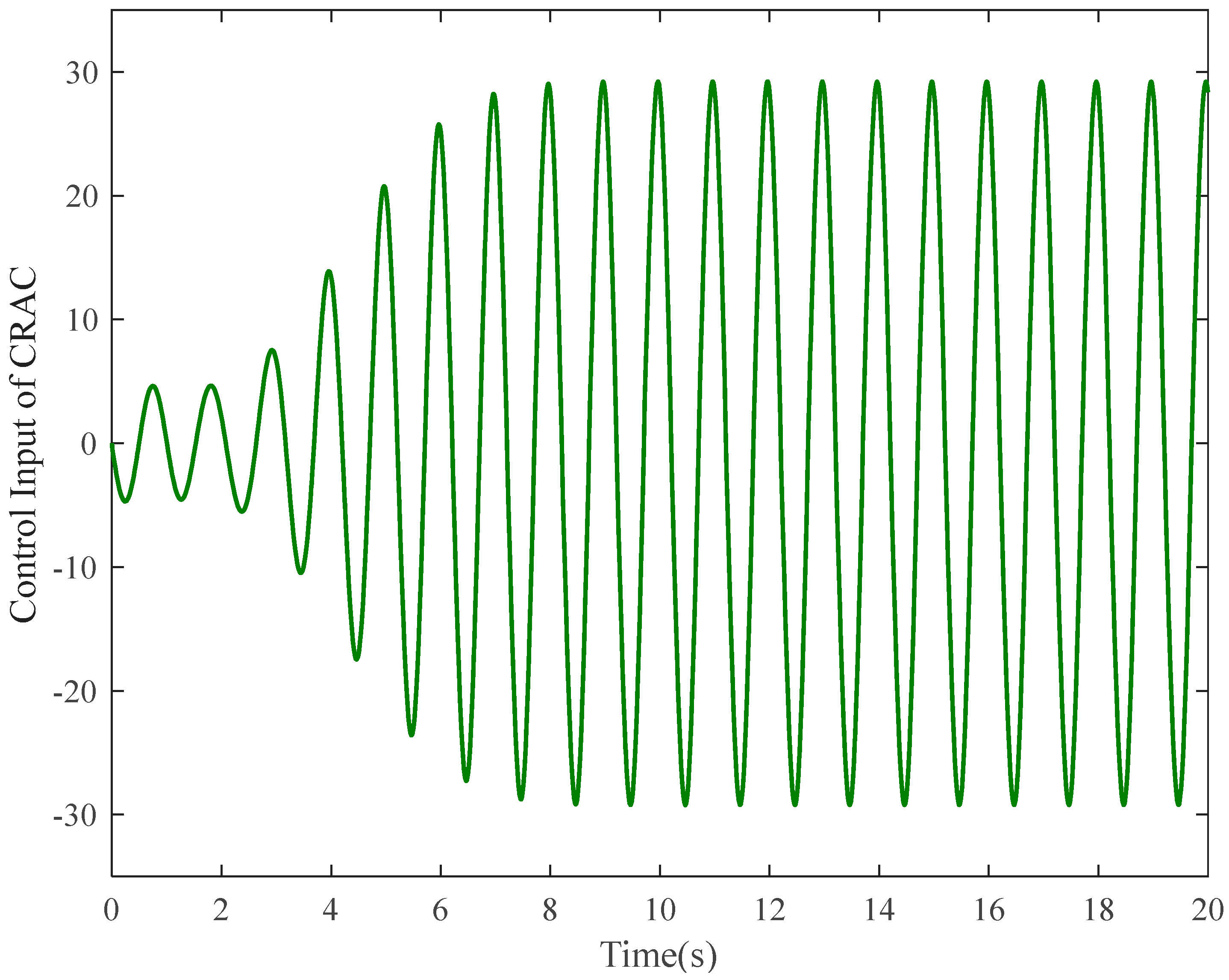
The tracking result of CRAC is given in Figure 1, which indicates that the x1 can track x1d closely. Additionally, the contrastive tracking errors of the employed three algorithms are exhibited on Figure 2. It is seen from them that the developed algorithm exhibits a better performance than others in aspects of transient as well as steady errors. It is worth noting that the proposed scheme performs the asymptotic tracking phenomenon since the tracking error gradually converges to zero. By comparing the performances of CRAC and CRC, the superiority of the NN compensations is indicated. Moreover, the robust performance of CRAC can be verified by observing the tracking results of CRC and CFC. In addition, the estimated performance of unknown functions with the CRAC algorithm can be seen from Figure 3, which shows that they are regular with bounded values. Moreover, the control input of CRAC is presented in Figure 4, which is smooth and bounded.
5. Conclusions
In this paper, several different robust neuroadaptive controllers that incorporate neuroadaptive control and nonlinear robust terms with a positive time-varying integral term have been integrated for the high-performance tracking of uncertain systems. Furthermore, the “explosion of complexity” caused by the traditional backstepping technology has been removed by utilizing the CFB design procedure. Specially, for each of the proposed controllers, an asymptotic tracking result for mismatched uncertain systems has been achieved. Comparative simulation verifications are achieved for an uncertain nonlinear system. The numerical results indicate the high-performance features of the presented controllers.
Funding
This research was funded by National Natural Science Foundation of China, grant number 52005249.
Data Availability Statement
No new data were created or analyzed in this study. Data sharing is not applicable to this article.
Conflicts of Interest
The author declares no conflict of interest.
Appendix A
Proof of Theorem 1 with Control Scheme I. Choose a positive function VL as the Lyapunov function candidate as
Taking the time derivative of VL, one yields
Substituting (8), (11), (15), (19) and (23) into (A2), one has
Moreover, we can rearrange (A3) as
Furthermore, one has
Based on (9), (10), (13), (14), (17), (18), (21) and (22), one obtains
Furthermore, we have
Applying Young’s inequality, one has
where
By adjusting γi and ωcj felicitously to keep the expressions in (A9) always positive, we have
where ρmin = min{kzi, kηi, kεj}.
By integrating both sides of (A10) for any time t > 0, one has
Along (A11), it shows that zi, ηi, , , and ∈L∞. With zi in (7) and the boundness of W, and , we can conclude ei, and ∈L∞. In addition, all system states are bounded because of the boundness of yr.
Depending on Lemma 1 and (9), one obtains
Therefore, φjs can be proven to be bounded due to the boundness of . Similar to (A12), we can achieve |βjs| ≤ and |us| ≤ . Thus, βi and u ∈ L∞.
Moreover, it can be concluded from (8), (11), (15), (19) and (23) that , and ∈ L∞. Hence ∈ L∞ can be gained. Finally, ei → 0 as t → ∞ can be derived according to Barbalat’s lemma, which ultimately confirms the Theorem 1.
Notably, proof of Theorem 1 with control scheme II or control scheme III can also be easily acquired according to the above steps. Here, we omit the relevant proof process.
References
- Yang, G.; Yao, J.; Ullah, N. Neuroadaptive control of saturated nonlinear systems with disturbance compensation. ISA Trans. 2022, 122, 49–62. [Google Scholar] [CrossRef] [PubMed]
- Yang, G.; Zhu, T.; Yang, F.; Cui, L.; Wang, H. Output feedback adaptive RISE control for uncertain nonlinear systems. Asian J. Control 2023, 25, 433–442. [Google Scholar] [CrossRef]
- Yao, B.; Tomizuka, M. Adaptive robust control of SISO nonlinear systems in a semi-strict feedback form. Automatica 1997, 33, 893–900. [Google Scholar] [CrossRef]
- Wang, X.S.; Su, C.Y.; Hong, H. Robust adaptive control of a class of nonlinear systems with unknown dead-zone. Automatica 2004, 40, 407–413. [Google Scholar] [CrossRef]
- Bechlioulis, C.P.; Rovithakis, G.A. Robust adaptive control of feedback linearizable MIMO nonlinear systems with prescribed performance. IEEE Trans. Autom. Control 2008, 53, 2090–2099. [Google Scholar] [CrossRef]
- Guo, L.; Cao, S. Anti-disturbance control theory for systems with multiple disturbances: A survey. ISA Trans. 2014, 53, 846–849. [Google Scholar] [CrossRef]
- Xu, Z.; Sun, C.; Hu, X.; Liu, Q.; Yao, J. Barrier Lyapunov function-based adaptive output feedback prescribed performance controller for hydraulic systems with uncertainties compensation. IEEE Trans. Ind. Electron. 2023; early access. [Google Scholar] [CrossRef]
- Chen, M.; Ge, S.S. Adaptive neural output feedback control of uncertain nonlinear systems with unknown hysteresis using disturbance observer. IEEE Trans. Ind. Electron. 2015, 62, 7706–7716. [Google Scholar] [CrossRef]
- Jiang, T.; Huang, C.; Guo, L. Control of uncertain nonlinear systems based on observers and estimators. Automatica 2015, 59, 35–47. [Google Scholar] [CrossRef]
- Chen, W.H.; Yang, J.; Guo, L.; Li, S. Disturbance-observer-based control and related methods—An overview. IEEE Trans. Ind. Electron. 2016, 63, 1083–1095. [Google Scholar] [CrossRef] [Green Version]
- Yang, G.; Yao, J. Nonlinear adaptive output feedback robust control of hydraulic actuators with largely unknown modeling uncertainties. Appl. Math. Model. 2020, 79, 824–842. [Google Scholar] [CrossRef]
- Tong, S.; Li, Y.; Sui, S. Adaptive fuzzy tracking control design for SISO uncertain nonstrict feedback nonlinear systems. IEEE Trans. Fuzzy Syst. 2016, 24, 1441–1454. [Google Scholar] [CrossRef]
- Zhang, Z.; Ju, H.P.; Shao, H.; Qi, Z. Exact tracking control of uncertain non-linear systems with additive disturbance. IET Control Theory Appl. 2015, 9, 736–744. [Google Scholar] [CrossRef]
- Zou, X.; Yang, G.; Hong, R.; Dai, Y. Chattering-free terminal sliding-mode tracking control for uncertain nonlinear systems with disturbance compensation. J. Vib. Control, 2023; early access. [Google Scholar] [CrossRef]
- Ying-Jeh, H.; Tzu-Chun, K.; Shin-Hung, C. Adaptive sliding-mode control for nonlinear systems with uncertain parameters. IEEE Trans. Syst. Man Cybern. Part B Cybern. 2008, 38, 534–539. [Google Scholar]
- Utkin, V.I.; Poznyak, A.S. Adaptive sliding mode control with application to super-twist algorithm: Equivalent control method. Automatica 2013, 49, 39–47. [Google Scholar] [CrossRef]
- Edwards, C.; Shtessel, Y.B. Adaptive continuous higher order sliding mode control. Automatica 2016, 65, 183–190. [Google Scholar] [CrossRef] [Green Version]
- Lee, J.; Chang, P.H.; Jin, M. Adaptive integral sliding mode control with time-delay estimation for robot manipulators. IEEE Trans. Ind. Electron. 2017, 64, 6796–6804. [Google Scholar] [CrossRef]
- Xian, B.; Dawson, D.M.; Queiroz, M.S.; Chen, J. A continuous asymptotic tracking control strategy for uncertain nonlinear systems. IEEE Trans. Autom. Control 2004, 49, 1206–1211. [Google Scholar] [CrossRef]
- Patre, P.M.; Mackunis, W.; Makkar, C.; Dixon, W.E. Asymptotic tracking for systems with structured and unstructured uncertainties. IEEE Trans. Control Syst. Technol. 2008, 16, 373–379. [Google Scholar] [CrossRef]
- Zhang, Z.; Xu, S.; Zhang, B. Asymptotic tracking control of uncertain nonlinear systems with unknown actuator nonlinearity. IEEE Trans. Autom. Control 2014, 59, 1336–1341. [Google Scholar] [CrossRef]
- Zhang, Z.; Xie, X.J. Asymptotic tracking control of uncertain nonlinear systems with unknown actuator nonlinearity and unknown gain signs. Int. J. Control 2014, 87, 2294–2311. [Google Scholar] [CrossRef]
- Liu, Y.H.; Li, H. Adaptive asymptotic tracking using barrier functions. Automatica 2018, 98, 239–246. [Google Scholar] [CrossRef]
- Liu, Y.H. Dynamic surface asymptotic tracking of a class of uncertain nonlinear hysteretic systems using adaptive filters. J. Frankl. Inst. 2018, 355, 123–140. [Google Scholar] [CrossRef]
- Cai, Z.; de Queiroz, M.S.; Dawson, D.M. Robust adaptive asymptotic tracking of nonlinear systems with additive disturbance. IEEE Trans. Autom. Control 2006, 51, 524–529. [Google Scholar] [CrossRef]
- Zheng, Y.; Wen, C.; Li, Z. Robust adaptive asymptotic tracking control of uncertain nonlinear systems subject to nonsmooth actuator nonlinearities. Int. J. Adapt. Control Signal Process. 2013, 27, 108–121. [Google Scholar] [CrossRef]
- Li, Y.X.; Yang, G.H. Adaptive asymptotic tracking control of uncertain nonlinear systems with input quantization and actuator faults. Automatica 2016, 72, 177–185. [Google Scholar] [CrossRef]
- Yang, G.; Yao, J.; Le, G.; Ma, D. High precise tracking control for a chain of integrator systems with modelling uncertainties. Trans. Inst. Meas. Control 2016, 39, 1710–1720. [Google Scholar] [CrossRef]
- Xu, B.; Sun, F. Composite intelligent learning control of strict-feedback systems with disturbance. IEEE Trans. Cybern. 2017, 48, 730–741. [Google Scholar] [CrossRef] [PubMed]
- Swaroop, D.; Hedrick, J.K.; Yip, P.P.; Gerdes, J.C. Dynamic surface control for a class of nonlinear systems. IEEE Trans. Autom. Control 2000, 45, 1893–1899. [Google Scholar] [CrossRef] [Green Version]
- Farrell, J.A.; Polycarpou, M.; Sharma, M.; Dong, W. Command fltered backstepping. IEEE Trans. Autom. Control 2009, 54, 1391–1395. [Google Scholar] [CrossRef]
- Yang, G.; Wang, H.; Chen, J.; Zhang, H. Command filtered robust control of nonlinear systems with full-state time-varying constraints and disturbances rejection. Nonlinear Dyn. 2020, 101, 2325–2342. [Google Scholar] [CrossRef]
- Liu, Y.H. Adaptive dynamic surface asymptotic tracking for a class of uncertain nonlinear systems. Int. J. Robust Nonlinear Control 2018, 28, 1233–1245. [Google Scholar] [CrossRef]
- Yang, G.; Yao, J.; Dong, Z. Neuroadaptive learning algorithm for constrained nonlinear systems with disturbance rejection. Int. J. Robust Nonlinear Control 2022, 32, 6127–6147. [Google Scholar] [CrossRef]
- Yang, G.; Wang, H.; Chen, J. Disturbance compensation based asymptotic tracking control for nonlinear systems with mismatched modeling uncertainties. Int. J. Robust Nonlinear Control 2021, 31, 2993–3010. [Google Scholar] [CrossRef]
- Wang, L.; Sun, W.; Su, S.F.; Wu, Y. Adaptive prescribed performance asymptotic tracking control for nonlinear systems with time-varying parameters. Int. J. Robust Nonlinear Control 2022, 32, 4535–4552. [Google Scholar] [CrossRef]
- Yan, B.; Niu, B.; Zhao, X.; Wang, H.; Chen, W.; Liu, X. Neural-network-based adaptive event-triggered asymptotically consensus tracking control for nonlinear nonstrict-feedback MASs: An improved dynamic surface approach. IEEE Trans. Neural Netw. Learn. Syst. 2022; early access. [Google Scholar] [CrossRef]
- Liu, Y.H.; Chen, L.L.; Zhou, Q.; Su, C.Y. Asymptotic output tracking control with prescribed transient performance of nonlinear systems in the presence of unknown dynamics. Int. J. Robust Nonlinear Control 2022, 32, 9363–9379. [Google Scholar] [CrossRef]
- Song, S.; Zhang, B.; Song, X.; Zhang, Z. Neuro-fuzzy-based adaptive dynamic surface control for fractional-order nonlinear strict-feedback systems with input constraint. IEEE Trans. Syst. Man Cybern. Syst. 2019, 51, 3575–3586. [Google Scholar] [CrossRef]
- Yang, G. Asymptotic tracking with novel integral robust schemes for mismatched uncertain nonlinear systems. Int. J. Robust Nonlinear Control 2023, 33, 1988–2002. [Google Scholar] [CrossRef]
Figure 1.
Tracking performance of CRAC.

Figure 2.
Tracking errors of CRAC, CRC and CFC.
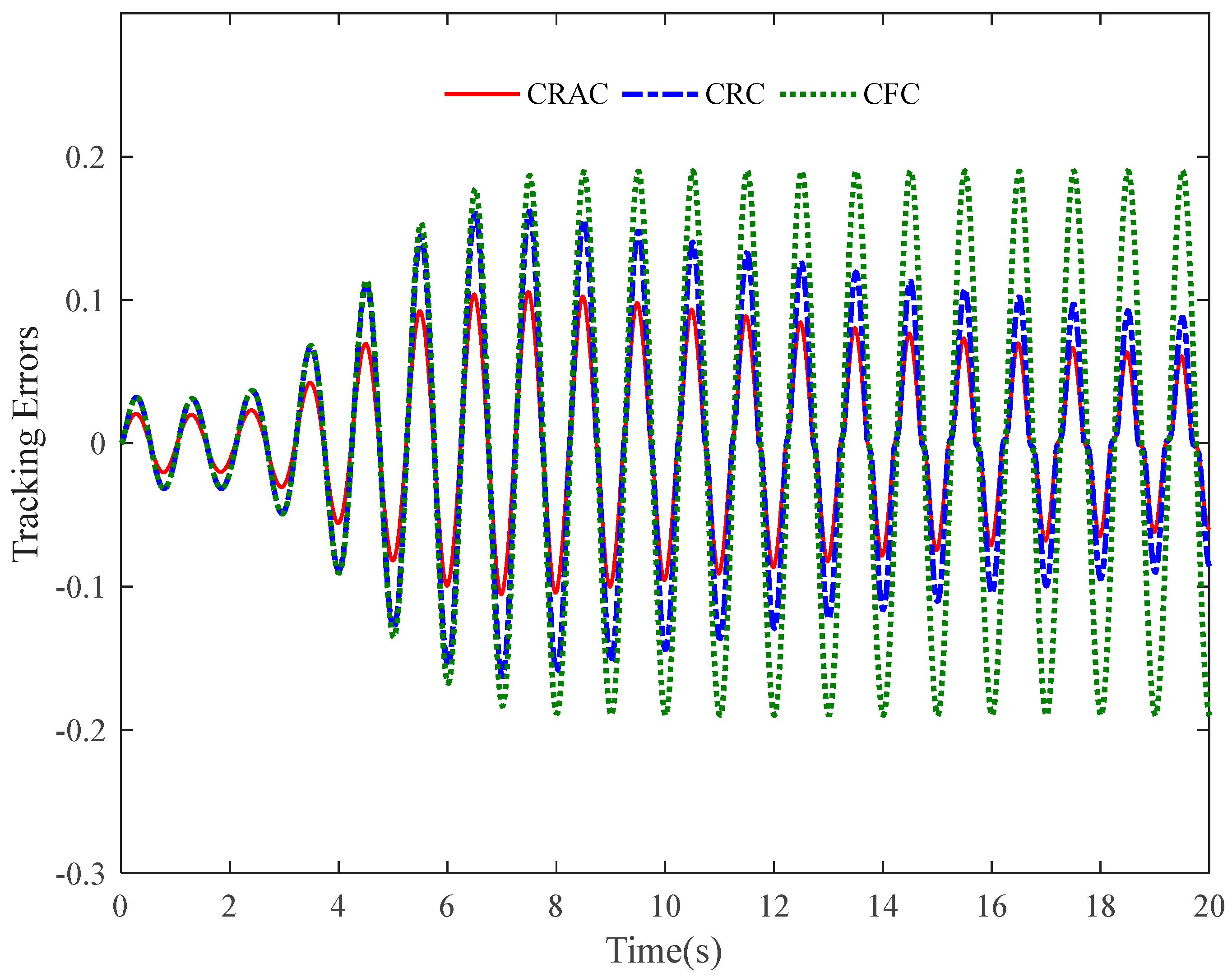
Figure 3.
NN estimation with CRAC.

Figure 4.
Control input of CRAC.
Disclaimer/Publisher’s Note: The statements, opinions and data contained in all publications are solely those of the individual author(s) and contributor(s) and not of MDPI and/or the editor(s). MDPI and/or the editor(s) disclaim responsibility for any injury to people or property resulting from any ideas, methods, instructions or products referred to in the content. |
© 2023 by the author. Licensee MDPI, Basel, Switzerland. This article is an open access article distributed under the terms and conditions of the Creative Commons Attribution (CC BY) license (https://creativecommons.org/licenses/by/4.0/).
Share and Cite
MDPI and ACS Style
Yang, G. Neuroadaptive Asymptotic Tracking Control of Nonlinear Systems with Multiple Uncertainties. Mathematics 2023, 11, 2978. https://doi.org/10.3390/math11132978
AMA Style
Yang G. Neuroadaptive Asymptotic Tracking Control of Nonlinear Systems with Multiple Uncertainties. Mathematics. 2023; 11(13):2978. https://doi.org/10.3390/math11132978
Chicago/Turabian StyleYang, Guichao. 2023. "Neuroadaptive Asymptotic Tracking Control of Nonlinear Systems with Multiple Uncertainties" Mathematics 11, no. 13: 2978. https://doi.org/10.3390/math11132978
Note that from the first issue of 2016, this journal uses article numbers instead of page numbers. See further details here.