1. Introduction
Most of the problems with uncertainties in our daily life can be modelled by fuzzy graphs. Fuzzy graph theory plays a salient role in making real connections between various objects in a system, with applications in network routing, wireless sensor networks, computer science, medical science, operations research, and more. In this introductory situation, the concept of fuzzy graphs provided by Rosenfield [
1] is presented as an interesting fuzzy mathematical tool in graph theory.
A tree cover of a fuzzy graph , denoted by , is the set of the minimum number of fuzzy trees as induced subgraphs that cover all the vertices of G. For a crisp graph, the tree cover number is approximated as the maximum positive semi-definite nullity as a conjecture. Although this graph parameter was first introduced as an essential tool in 2011, there is very little information in the existing literature.
For minimizing the maximum cost of a tree cover, we are interested in finding a tree covering of a fuzzy graph with at most s number of trees which span the whole graph, as it is known that constant factor approximations to travelling salesperson tracks can be used to find the minimum number of spanning trees.
The actual purpose of the facility location problem is to decide which node to allocate to a set of facilities in order to provide full coverage to the service needed for several demand nodes in a system in the most efficient way. In addition, a customer or demand point may decide on the location of their facility nodes to cover the demand needed by every customer in the fuzzy network. Nowadays, one of the crucial problems is the placement of servers or data objects in any communication network to ensure that the latency of access is optimized. However, the primary purpose of the problem is always the same; the aim is to maximize the profit, that is, to minimize the allocation costs of different facility nodes in the system.
Many facility location problems include possible locations for facility nodes to be built on or opened at already-built facilities. In this case, information about the building or opening cost for a facility in that location is supplied. A set of demand nodes or customers can be considered, with detailed information about the amount to be covered and the connection cost between the demand point and a certain facility point. On the other hand, many conditions or restrictions in a facility’s location problem need to be satisfied. An objective function which needs to be optimized is always present in such problems. One objective function is generally based on the cost, which includes all types of costs, such as demand, ordering, transportation, etc., for all system facilities.
In certain facility location problems, a profit can be associated with the assignment, then the objective profit function is optimized. One critical way of characterizing the facility location problem is on the basis of whether the facilities in the system are of variable-covering radius or fixed-covering radius in terms of how many demand nodes are to be covered by a facility within its covering radius. This kind of facility location problem is difficult to solve; we handle such problems in this article.
Now, we have to go through the rich literature on covering problems, which is the main topic of work within this article. The tree covering problems modelled and solved in this article are closely associated with the works of Arkin, Hassin, and Levin [
2], who have dealt with various covering problems, including coverage of vertices for a crisp graph and a subset of edges of a graph with a partition in walks, paths, or stars. There are a variety of studies on approximation algorithms to minimize the number of objectives for covering purposes (such as paths) by satisfying some restrictions on the cost of each covering object.
An efficient feasible solution includes
k-tours for covering the vertices of a crisp graph in the
k-traveling salesperson problem. The main objective in this model is to minimize the total tour length. It is possible to partition all vertices of a graph into several clusters, and the weight of a star or low-cost spanning trees in the cluster is considered the weight of the cluster in that graph. Rana et al. [
3] worked on unweighted interval graphs with conditional covering problems (CCP). In addition, Bhattacharya and Pal have presented works on different types of covering problems involving fuzzy graphs [
4,
5,
6,
7].
Mordeson and Peng [
8] discussed concepts around various operations on fuzzy graphs. Samanta and Pal [
9] have provided results on the fuzzy colouring of fuzzy graphs and fuzzy tolerance graphs. Fuzzy planar graphs with
m-polarity are discussed in the work of Ghorai and Pal in [
10]. Cardinal and Hoefer [
11] have worked on various types of covering games. Chang and Zadeh handled fuzzy mappings and control techniques in [
12]. Chaudhry introduced new heuristics for solving CCP in [
13]. Chen and Chen [
14] have provided a new method of finding similarity measures between two fuzzy numbers. Ghorai and Pal [
15] have studied faces and dual
m-polar fuzzy graphs. Jurji and Borut combined research on the facility location and covering problems in [
16]. Fuzzy graphs were used in network optimization by Koczy [
17]. In a similar way, Hakimi [
18] worked on communication networks. The problem of emergency service facility location was handled by Toregas et al. [
19]. Related problems on fuzzy graphs were studied and solved by Bhattacharya and Pal in [
20].
Nayeem and Pal [
21] solved the shortest path problem on a network. Ni [
22] worked on a research area involving covering problems of edges having minimum weights. Pal et al. [
23] detailed new ideas with respect to modern trends in fuzzy graph theory. Pramanik et al. [
24] discussed interval-valued fuzzy planar graphs. A study on bipolar fuzzy graphs was revealed by Rashmanlou et al. in [
25]. The research area of Samanta et al. in [
26] included vague graphs and their strengths.
The motivation for the present article arises from the “Doctor station location” problem. Consider the problem of a hospital that requires s doctors to be located in the campus area for total coverage. A single doctor can be assigned to a particular number of patients, and the doctors make their rounds in shifts during the morning. The purpose of the problem is to find suitable locations for doctor stations and determine how to cover the requirement of treating every patient in such a way that the time for completing the entire process is minimized. Similar types of real-life problems motivate us to use the concept of tree covering in a modelled graph.
The “doctor station location” problem is similar to the problem of covering a graph with at most k number of tours while maintaining the minimum value of the maximum length of a tour. A constant factor approximation for a minimum number of trees spans the whole graph of travelling salesperson tours. We are interested in finding a covering of the graph with at most k number of spanning trees and the minimum value of the maximum weight of those trees. When a doctor must return to their station to pick up necessary supplies without first visiting every patient, a variation occurs in the considered problem. At such a point, the problem of covering the graph is formulated with the help of stars in the graph. In addition, we can consider the possibility of the hospital already having been built with all required doctor stations, in which case we only need to find the best possible way of assigning patients to doctors. Thus, these problems are transformed into the problem of finding rooted trees that covering the graph.
The idea described above inspires us to deal with tree-covering problems; for a realistic level of imprecision, we include the flavour of fuzzy graphs in this article. In addition, we chose the banking system as a case study in the application part, keeping in mind the importance of a developed model in solving real-life problems involving a combination of the facility location problem and tree covering of fuzzy graphs. The need to address such circumstances and situations influence our construction of a model with three optimization programming problems.
The main contributions in the sense of covering problems and real-life implications are organized in this portion. There are two variations of the facility location problems, one in which the covering radius is fixed for all facility vertices and one in which the covering radius differs for the vertices of different facilities. Earlier works have addressed covering radius variations and solved related problems involving a particular type of covering radius. However, it is more practical to have the number of demand points be saturated by a particular facility vertex of a fuzzy network depending on the covering radius type.
The contributions of this paper can be summarized as follows:
- (i)
This paper is the first to handle the two cases of a fixed covering radius and variable covering radius simultaneously in one model. The concept behind our proposed model is intended to cover all demand vertices. In this paper, we solve such complex facility location problems by minimizing the number of facility vertices, minimizing the total cost for all demand vertices, and maximizing the demand saturation of facility vertices. All fuzzy solutions for the model are determined using ‘LINGO’ mathematical software 18.0.44.
- (ii)
We introduce new definitions of tree cover and tree covering numbers for a fuzzy graph, design an efficient algorithm to determine the number of rooted trees s needed to cover a fuzzy graph, and present the algorithm’s complexity analysis.
- (iii)
In the application part, we analyze the Indian banking system using our developed model and algorithm. As an outcome of this real-life application, the conclusion is reached that the number of small denominators (up to INR 100) is minimized. The cost required to maintain the flow of denominations for the Indian banking system is thereby minimized. Lastly, the demand saturation of denominations at the bottom level is assessed in the interest of economic freedom.
This article includes the following sections, excluding the present introduction. In
Section 2, necessary definitions and concepts are provided. The covering problem considered in this article is described in
Section 3 with the mathematical formulation.
Section 4 illustrates the mathematical formulation of the developed model.
Section 5 illustrates the model with a suitable example. A real-life application involving emergency aircraft landing situations is analyzed using the proposed model in
Section 6. Finally, our overall conclusions are provided in
Section 7.
2. Preliminaries
Several basic definitions and necessary aspects are provided in this portion of the paper. These parameters are beneficial in developing the model for a fuzzy graph with a facility location concept.
Here, all the components of a triangular fuzzy number (TFN) are normalized, i.e., between 0 and 1. Different types of scaling are used for the normalization process in different situations. Additionally, the format of the TFN with the representation of its components as in Definition 1 is followed throughout the article.
Definition 1 ([
4]).
Let be a TFN that has the following function as its membership function:Then, the defuzzified form of is denoted by , defined as Definition 2 ([
8]).
A fuzzy graph is a non-empty set which carries two functions, and , for all , where σ is the vertex-membership function and μ is the edge-membership function satisfying . Definition 3 ([
4]).
A set of vertices of a fuzzy graph is said to be a fuzzy vertex cover of G if each vertex of is incident to every edge of G within a fuzzy covering radius . Definition 4. Consider a fuzzy graph . A coverage radius of G is defined as a predefined number which reflects a distance in G. If for an arbitrary vertex u of G, then this vertex v is covered by u in fuzzy graph G.
Definition 5. Let G be a crisp graph and let be a collection of subgraphs of G where is a tree for all . If exists for every edge such that , then is a tree cover of G.
Definition 6. The tree covering number for a crisp graph G is provided by Definition 7. Let be a fuzzy graph and let be a collection of subgraphs of G where is a fuzzy tree for all . If there exists for every edge with in G such that in , then is a tree cover of fuzzy graph .
Definition 8. The tree covering number of a fuzzy graph is provided by 2.1. Notations and Symbols
This part clarifies all the necessary notations to signify the quantities used in the entire paper in deducing the theories. The symbols and their meanings are provided in tabular form in
Table 1.
2.2. Problem under Consideration
Consider a fuzzy graph , where V is the set of vertices. There are three types of vertices in the graph: facility vertices, demand vertices, and free vertices. The free vertices are neither demand vertices nor facility vertices. The graph is assumed to contain some demand and facility vertices, while the free vertices may or may not exist. The facility vertices can store commodities (such as food, water, weapons, etc.) required for emergency or regular distribution. These vertices may be hospitals, military camps/offices, ration shops, or distribution centres. Demand vertices take such commodities for use, and generally represent people, organizations, etc. Free vertices are neither demand vertices nor facility vertices. Thus, new facility vertices may be initiated with respect to any free vertices. Because these vertices have no demand, free vertices cannot be considered demand vertices.
There are two possible cases. The first is that all the demand vertices are covered by at least one facility vertex (i.e., the required demand is fulfilled by any one of the facility vertices), regardless of the cost or distance to reach the facility. In the second case, certain demand vertices are not covered by facility vertices (as the demand vertices may be far away from facility vertices, or transport or other costs may be too high).
In both situations, we insert more facility vertices to reduce the cost, distance, etc. It is assumed that each facility vertex may cover all the demand vertices within a specific circular region (i.e., provide the commodities to the demand vertices). The radius of this circular region is called the covering radius. This radius may be the same for all facility vertices (i.e., fixed) or different for different ones. In this case, the covering radius is variable or dynamic.
Many parameters or situations may arise with respect to constructing new facility vertices. Here, we select the free vertices as facility points under different assumptions, objectives, and constraints.
The main assumptions are:
- (a)
The building cost for a facility point at an arbitrary vertex (say, i) can be taken as (a fuzzy number).
- (b)
If a customer at vertex k has decided to take services from a facility point (at i), then a cost (a combination of the establishment cost, ordering cost, and transportation cost) is imposed on the demand point.
- (c)
There are two types of covering radius: the first is a variable covering radius in which each facility serves unlimited customers, i.e., the covering radius is flexible depending on the situation, while the second is a fixed covering radius in which each facility can serve a maximum (say, u) number of demand points.
The objectives of our model are as follows:
- (a)
Minimize the total number of facilities.
- (b)
Minimize the total cost for all demand points.
- (c)
Maximize demand saturation by the facilities.
We use the following constraints or restrictions:
- (a)
The total number of facility nodes must be less than or equal to the maximum number of locations allocated in the fuzzy graph.
- (b)
The sum of the value of supplying a service by an arbitrary facility point i to a customer at demand point j is assumed to take a fixed value (say, M).
- (c)
The total demand cost in a certain period (say, ) is less than or equal to the total servicing cost in the fuzzy network.
- (d)
The servicing cost paid by an arbitrary demand point i is always a positive amount.
- (e)
The upper limit of the covering demand cost is the product of K and , where K is the maximum number of possible vertices (locations) allocated in a fuzzy graph G and is the approximate number of days needed by a facility vertex i to saturate demand with respect to a demand vertex j, with j being a fuzzy number.
- (f)
The flexibility of a facility point j in terms of providing facilities is less than or equal to the amount of the covering demand.
- (g)
There should always be a non-zero day for ordering demand and providing facilities from a facility point.
3. Problem Description
In this portion, the considered covering problem in a facility location model is described in a broader sense. A simple connected fuzzy graph is taken as an example throughout this article. The covering radius for the facility points is taken as a fuzzy number. In a system with fuzziness, distances and other types of costs are taken as fuzzy numbers as well.
Our model assumes that the resulting fuzzy system has two types of facility nodes.
(i) Facility location problem with variable covering radius. For the variable covering radius case, the following problem is considered: let be a possible set of locations, and let for be the distances between them. For possible choices of points to open a facility, for each location , a subset is supplied, while for opened facility points a subset is assigned to the demand points. Corresponding to every location , the non-negative cost is assumed at location i. In addition, is the cost of demand location j assigning an opened facility point at i per unit of demand.
It is assumed that these costs are symmetric and non-negative fuzzy numbers and that they satisfy the following triangular inequality:
for all and for all .
To minimize the total cost, finding a feasible assignment to an open facility point of every location in the set D is required.
(ii) Facility location problem with fixed covering radius. In this case, we consider the situation where every existing facility point produces a total demand less than or equal to a positive integer. It is interesting to investigate whether we can prove that the adaptive covering radius in our developed algorithm affects the capacity of the facility location problems for finding the tree cover of a fuzzy graph and solving facility location problems with a fixed covering radius.
When the optimal value of the total demand is given in the variable covering radius type, the trivial problem is finding the corresponding facility points for the fuzzy graph. In this case, anyone can assign each location to the location i such that provides the minimum value among all possibilities ensuring that .
There is sufficient capacity for the fixed covering radius to saturate the total demand occurring in a fuzzy system. Two variants of facility location problems exist in our consideration. The situations are selected depending on the demand condition for each vertex of the fuzzy graph. An arbitrary facility point is allocated for only one demand point, or the facility point is fractionally split among more than one demand point in the system.
First, we must determine the type of the problem, i.e., whether it is of variable or fixed covering radius type. Then, we need to find an arrangement to ensure that there is a route to a facility point by optimizing all parameters. For example, we can take the amount of demand at each demand point together with an integer value representing the upper bound of demand for a particular problem. A minimum cost assignment is determined if the optimum value for total demand is supplied. In every problem, the presumption is that corresponding weights (edge weights and vertex weights) for facility points are provided.
To solve the considered problem, one crucial task is to find a tree cover of a fuzzy graph with an optimized cost different from the problem. In the next portion, we design an algorithm for finding such a tree cover.
3.1. Algorithm to Find Rooted Trees Covering Fuzzy Graph G
The bin packing problem is an optimization problem in which items of different sizes must be packed into a finite number of bins or containers, each of a fixed capacity and depending on the covering radius, in a way that minimizes the number of bins used. Generally, a BIN-PACK Algorithm refers to an approximation algorithm used to solve the above bin packing problem.
In this portion of the paper, we modify an existing BIN-PACK algorithm designed for crisp graphs for use with fuzzy graphs. We briefly describe the FUZZY-BIN-PACK Algorithm used to find a tree cover for the fuzzy graph with an optimized cost of at most . It should be noted here that the set of vertices for locating the facility/demand points is treated as a collection of elements in our modified algorithm.
In Algorithm 1, we take a fuzzy graph
with vertex and edge costs as input. We provide a fixed capacity
A for a fixed covering radius case of facility vertices (i.e., bin capacity) for the given graph. We aim to find a tree cover of
G with an optimized cost of at most
. In the first step, we compare the cost of any arbitrary vertex with
A. If the cost is higher than
A, we remove it from the vertex set of
G. Next, we find a spanning tree with a minimum size in
G, a transformed version of
G when the roots in a given sample set
S of vertices to be either facility or demand nodes are contracted to a single vertex. Then, we collect all uncontracting from the minimum spanning tree and obtain forests
for
. Now, to decompose the edges of each forest, we can find trees and an individual component such that the cost of the obtained trees must belong to
and the cost of the other portion must be less than the fixed bin capacity
A. In the next step, if the distances from the obtained trees to an arbitrary vertex of
G are less than or equal to
A, we check whether the trees are subgraphs or not for all possible cases. If all trees are not subgraphs of
G, then we can conclude that the considered bin capacity is too low in cost; in this case, the process is repeated after modifying the value. On the other hand, if every tree is a subgraph of
G, a success statement is returned for the choice of this bin capacity in obtaining an optimized tree cover of
G. Finally, we obtain a set of trees which are all subgraphs of
G for which the number of roots of these trees is finite, i.e., a tree covering with optimized bin capacity for the facility and demand vertices of the given fuzzy graph with finite size.
| Algorithm 1: FUZZY-BIN-PACK. |
- Input:
A fuzzy graph with associated costs to the vertices and edges. Also, a fixed bin capacity ‘A’ and a sample set S of vertices for choosing as facility and demand vertex are given. - Output:
A tree cover for the fuzzy graph with the optimized cost at most . - Step 1:
If , then for any arbitrary . - Step 2:
For a fuzzy graph , find (spanning tree with minimum size) of G which is a transformed version of G when the roots in S are contracted to a single vertex. - Step 3:
In S, un-contracting roots from ; obtain a forest for . - Step 4:
Decompose edges of each tree into trees such that , for every j and . - Step 5:
If for any arbitrary vertex . Check whether is a sub-graph of G for all j. - Step 6:
If not all trees are sub-graph of G, then Return failure: “A is a too low cost”. - Step 7:
If every tree is a sub-graph of G, then Return to success and go to step 8. - Step 8:
Get a set of trees where each tree consists of , a sub-graph of G, the number of roots is s, and the tree N (if any) in leftover, which contains the fuzzy root graph G, denoted by r.
|
.
3.2. Complexity Analysis of the Proposed Algorithm
We next explore the complexity analysis of our proposed FUZZY-BIN-PACK algorithm. In this algorithm, we fix the bin capacity to cover the whole fuzzy graph with the help of trees by limiting the cost to most four times the bin capacity, as per our previous considerations. If there are n number of vertices with non-zero membership values in the fuzzy graph, then the cost verification for the total number of vertices takes times. In the next step, if there are m numbers of contracting roots in S to find a connected tree it takes times, as this is the most generalized possibility for finding trees to make a tree cover. For other situations, every tree needs to be checked to determine whether it is a subgraph of the considered fuzzy graph G by verifying the tree’s distance from any arbitrary vertex of the main graph. For this purpose, the required time is . Therefore, the total time required to perform the proposed algorithm is . Thus, the time complexity of our proposed FUZZY-BIN-PACK algorithm is .
3.3. Advantages of Proposed Algorithm
In brief, the approximation algorithm known as BIN-PACK can be used to solve problems related to precise data. This algorithm helps to find the minimum number of total bins needed to assign each item to a bin when considering a finite number of items of different weights and a fixed capacity of bins in the system. This is useful in finding the minimum number of facility vertices needed to saturate all the demand in a system with crisp data and parameters, i.e., it is helpful for crisp graph scenarios under a graph-theoretical approach.
Practically, however, such crisp models have little relation ro real-life problems which involve several imprecise data types. Suppose that the number of the bins is not fixed; in this scenario, the existing algorithm is not applicable, as it cannot find any parameter with fuzziness. More clearly, it is obvious that in any network the accessible amount of facilities and order of demand are uncertain, and depend on various circumstances within the system. Therefore, it is notable that fuzzy graphs are a more practically justified tool for modeling realistic problems. In these cases, the existing BIN-PACK algorithm fails to compute the solution due to the need to handle fuzzy parameters. These more complex situations motivate us to modify the BIN-PACK algorithm for fuzzy environments and develop our proposed FUZZY-BIN-PACK algorithm. A complexity analysis of the proposed modified algorithm is provided in
Section 3.2.
4. Mathematical Formulation
In this article, we consider fuzzy systems modeled as fuzzy graphs. If any uncertain or vague parameters are present in any system, it can be described as a fuzzy environment. Vertices are chosen as facility or demand vertices based on the relevant information of a particular case. It is obvious that in real life the available facilities and possible demand must be imprecise. Thus, the vertices are fuzzy with regard to their respective membership functions. Here,
represents the number of fuzzy vertices that are facility vertices; on the other hand,
represents the amount of demand saturation by facility nodes. It is assumed in the model that the maximum possible number for allocating demand or facility nodes is
K. The other notations and their proper meaning in the proposed model are provided in
Table 1. Next, we move through the mathematical formulation of objective functions subject to all conditions in the model to find the solution of the problem described in
Section 2.2.
The main objectives of the developed model are as follows:
- (i)
To construct the first objective function, we multiply the number of facilities
n by the corresponding fuzzy variable
representing potential locations of facility vertices. Meanwhile, several demand points
m are multiplied by the fuzzy variable
to represent demand saturation of the demand vertices. The operational cost is incorporated in the calculation of the facility vertices through multiplication by the parameter
. In this way, the total number of facility and demand nodes provided by
is minimized.
- (ii)
The second objective function related to total fuzzy cost is constructed by taking the difference between two quantities, the first representing the product of the minimum number of days among
needed to saturate demand in the fuzzy network based on the amount of fuzzy cost
paid by the facility node for transportation and the second representing the product of the fuzzy cost
paid for demand ordering, where the maximum possible number for allocating demand or facility nodes in the network is
K. Therefore, we seek to minimize the total cost, which is represented by
- (iii)
The last objective function seeks to maximize the total demand saturation of the fuzzy network. The demand saturation of the network depends on the tree covering number corresponding to the tree coverage of the network, the fuzzy transportation and ordering costs, the fuzzy weights associated with demand, and the number of facility points
M for facilities available in the network. Thus, this objective function involves four expressions: the first for fuzzy cost, the second for tree covering number
, the third corresponding to the fuzzy weights
, and the last for the available facilities. Therefore, we seek to maximize the demand saturation, as follows:
The above-described functions are optimized in our model subject to certain conditions that need to be satisfied. The constraints subjected to these objective functions are as follows:
- (a)
The total number of facility nodes must be less than or equal to the maximum number of locations that can be allocated in the fuzzy graph
- (b)
The sum of the value of supplying services from an arbitrary facility node
i to a customer at demand point
j is assumed to be a fixed value (say,
M):
- (c)
The amount of total demand cost in a certain period (say,
) is less than or equal to the total servicing cost in the fuzzy network:
- (d)
The servicing cost paid by an arbitrary demand node
i is always a positive amount:
- (e)
The upper limit of the covering demand cost is the product of
K and
:
for
.
- (f)
The flexibility amount when a facility node
j provides facilities is less than or equal to the amount of the covering demand
- (g)
There should always be a non-zero day for ordering demand and for a facility node to provide facilities:
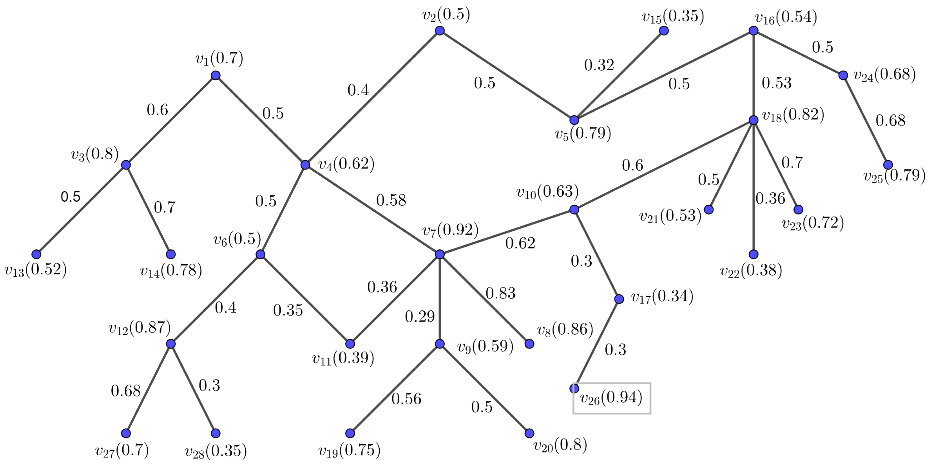
5. Example Illustration
This section illustrates use of the proposed model for the fixed covering radius case of the fuzzy graph
in
Figure 1 along with its vertices and corresponding edges. In this section, the parameters taken as fuzzy numbers in the description of the problem, such as the covering radius, distances, weights, and the costs corresponding to the vertices and edges of the fuzzy graph, are triangular fuzzy numbers. The proposed model can be illustrated using other types of fuzzy numbers as well.
In this example, the fuzzy graph
in
Figure 1 with 26 vertices and 29 edges and their corresponding membership values, weights, and fuzzy costs is taken as an example. All of the weights and costs are triangular fuzzy numbers. We assume that all required data are supplied in
Table 2.
To assign the edge membership values in the fuzzy graph, it is maintained that
for any arbitrary vertices
u and
v in
.
Using our developed algorithm, we can find a tree cover for the considered fuzzy graph as follows:
where
The programming problem denoted as Problem 1 of the constructed model with three objective functions and associated conditions is provided as follows:
Problem 1.
Subject to constraints
for
for
We assume the following for this example:
for the payment situation of demand point j with respect to facility point i.
is the approximate number of days needed by facility node i to saturate the demand of demand node j=(0.58, 0.65, 0.79).
is the fuzzy amount to be determined; it is the approximated cost paid at facility node i for transportation.
is the fuzzy cost paid for demand ordering by demand point j = (0.79, 0.82,0.95).
is a fuzzy variable used to identify many facility nodes in a fuzzy network, which is a fuzzy number.
is a fuzzy variable used to identify many demand nodes in a fuzzy system.
It is defined that .
Now, we have to evaluate the values corresponding to the trees , respectively, in the tree covering set of G.
, which corresponds to the tree . Thus, we have to calculate the total summed weight of the tree for the tree covering number of G.
Therefore,
.
In addition, the maximum fuzzy limit of the total amount of facilities supplied in the fuzzy system is .
By solving the programming problems of the model with the help of the mathematical software 18.0.44 ‘LINGO’, the variables to be determined are , , , m and n. These are all fuzzy parameters, and are taken as triangular fuzzy numbers in this illustration. Then, Problem 1 is reduced to Problem 2 below.
Problem 2.
Using ‘LINGO’ mathematical software, we obtain the following solutions for these programming problems.
, , , , . The minimum number of approximate choices for facility nodes is , the minimized total fuzzy cost for the fuzzy network is , and the maximized demand saturation concerning weights and fuzzy costs is .
6. Example Application
The recent COVID-19 pandemic has caused an abnormal situation for the global economy due to complicated circumstances such challenges within of the banking system and other financial institutions. In the Indian banking system. there is an ongoing revolution in the operations and services of banks and financial institutions due to the incorporation of new and updated technologies.
The Reserve Bank of India functions as a sunshade for the entire Indian banking industry, being responsible for the central banking system and regulatory processes. There are two types of banks in the Indian banking system, namely, commercial banks and co-operative banks.
At present, different opportunities and challenges are faced by the Indian banking system. According to the Annual Report of the RBI, the main opportunities and challenges of the banking industry lie in continued development of the banking process to sustain the Indian banking system while reducing bankruptcies and other negative parameters.
Compared to the previous year, the level of consumer awareness is significantly higher. Today, consumers need internet banking, mobile banking, and ATM services with high frequency and reliability.
In the banking system, the optimal number of banknotes per denomination is not certain, and varies per year according to the annual report of the Reserve Bank of India. Any banknote denomination can be represented with the help of many other banknotes, a relation that is imprecise and varies over time. Thus, a great deal of vagueness and uncertainty exist in the banking system, and problems related this can be represented and solved with the help of fuzzy graphs. To construct a fuzzy graph related to this system, it is first necessary to choose proper vertices and edges; this selection process is described in the next portion.
6.1. Construction of Fuzzy Graph
In the last part of 2020–2021, the number of soiled banknotes needing to be disposed of was severely affected by the COVID-19 pandemic, a phenomenon that was expedited slowly in order to maintain a stable economic structure. Thus, there was a 32% decline in the disposal process of soiled banknotes in that financial year compared to the previous year.
Following the annual report of the Reserve Bank of India at the end of March 2021, here we consider the denominations of banknotes as vertices of a fuzzy graph. To assign vertex membership values, we first observed the denomination of banknotes from 2019 to 2021. Then, we took the average as the mean value of a triangular fuzzy number (TFN). The fuzzy graph uses these triangular fuzzy numbers as vertex membership values. On the other hand, if other banknotes can represent any banknote, then an edge exists between those vertices corresponding to the same banknotes. For example, there is an edge between the vertices corresponding to banknotes with values of INR 100 and 500. In addition, the vertex membership values are used to assign edge membership values in the fuzzy graph.
First, we must find the average percentage of parameters which affect the banking system, then turn this into a triangular fuzzy number. These TFNs are used to find similarity measures with the vertex membership values in order to determine the corresponding fuzzy weights for each vertex in the constructed fuzzy graph. The cost is taken as a fuzzy number representing the difference between denominations in the year 2021 and the denominations’ averages corresponding to their vertices. Here, the facility points are assumed to be the smaller denominations and the demand points are to be taken as larger denominations. The edge membership values in the fuzzy graph must maintain the following:
After constructing the fuzzy graph, we have to find a fuzzy tree cover and its tree covering number, then proceed to find the objectives and constraints of this particular part of the example. We aim to find the minimum number of smaller banknote denominations, minimize the fuzzy cost in the Indian banking system, and maximize demand saturation with respect to banknote circulation.
6.2. Case Study
At 21.4 percent of GDP for the end of December 2020, India’s external debt remained lower than that of its emerging-market peers. The external vulnerability indicators at the end of March of 2021 are listed in
Table 3, which reflect the approximate percentage unless indicated otherwise.
The number of frauds reported during the financial year 2020–2021 decreased by 15% in terms of number and 25% in terms of value. There was a decrease in the share of PSBs in terms of both value and number among the total number of frauds concerning private sector banks during the corresponding period.
Banknotes in Circulation
During 2020–2021, there were increases of 16.8% and 7.2% in the value and volume, respectively, in the circulation process of banknotes. The highest share in volume terms is for the INR 500 denomination, whereas the lowest is for INR 10 banknotes, as of 31 March 2021.
Table 4 shows the details on banknotes in circulation to the end of March of 2021.
The fuzzy graph constructed using all these data is shown in
Figure 2.
6.3. Formulation of the Problem
In this application area of our developed model, we have taken the Indian banking system as a fuzzy network, considering banknote denominations as items to be supplied from the facility to the demand vertices. The tree-like flow of denominations from the Reserve Bank of India to the common people helps in modeling such a system using the concept of tree cover in a fuzzy graph. The main problem is to minimize the number of small denominations without affecting the flow of demand in the lower layer related to the market level. For this purpose, we can use our proposed model with appropriate assumptions related to the Indian banking system to find all the solutions to the problem. The specific assumptions and considerations are described in the following portion.
Our objective for this application using the proposed model is to minimize the approximate number of smaller denominators (Obj 1), minimize the approximate total fuzzy cost in the Indian banking process concerning the corresponding weights mentioned earlier (Obj 2), and maximize demand saturation with respect to the economic need of the people through circulation of banknotes in the Indian economic system while accounting for external vulnerability indicators (Obj 3).
For this application, the data are as follows.
for the payment situation of the larger denomination j with respect to the smaller denomination i.
is the approximate number of days needed to saturate demand using a small denomination i with respect to a larger denomination j = (8.78, 9.35, 10.59).
is a fuzzy amount to be determined, representing the approximate cost of a smaller denomination i for transportation from one bank to another.
is a fuzzy cost paid for demand ordering due to circulation of the larger denomination j = (8.29, 9.32, 12.57).
is a fuzzy variable used to identify a number of smaller denominations in the fuzzy banking system, and is a fuzzy number.
is a fuzzy variable used to identify the number of larger denominations in the fuzzy banking network.
It is defined that
, where
and
, which corresponds to the tree
. Thus, we have to calculate the total summed weight of the tree for the tree covering number of
G.
Therefore, .
In addition, the maximum fuzzy limit of the total amount of facilities supplied in the fuzzy system is .
By solving the programming problems of the model using ‘LINGO’ mathematical software, the variables to be determined are , , , m, and n. In this illustration, all of these fuzzy parameters are taken as triangular fuzzy numbers.
6.4. Solution of Programming Problems
Then the problem Problem 1 is reduced to the problem, namely Problem 3 given by the following.
Problem 3.
Using the mathematical software ‘LINGO’, we have the following solutions for these programming problems.
= (5.78, 6.84, 8.97), , , , . The minimum number of approximate choices for facility nodes is , the minimum total fuzzy cost for the fuzzy network of the banking system is , and the maximum demand saturation concerning the weights and fuzzy costs is .
6.5. Insightful Analysis
Based on the solutions obtained by the model in this application scenario, we can conclude the following:
- (i)
The minimized number of total small denominations (i.e., banknotes of INR 2, 5, 10, 20, 50, and 100) provide a total coverage in the RBI banking system of , which is a fuzzy volume, i.e., in lakh; that is, a minimum total number of new banknotes of 9.27 lakh to 9.23 lakh per year in denominations of INR 2 to 100 need to be supplied for a smooth flow of denominations in the optimized sense, with the best results occurring for the case of 9.86 lakh.
- (ii)
The minimized total fuzzy cost in the fuzzy system representing the banking process is (in volume, i.e., INR notes in lakh) for smooth circulation of banknotes in the coming financial year to sustain the economic development of India. This objective function reflects the minimum denomination number needed to calculate cost for maintaining flow in the Indian banking system per year, and ranges from 14.38 lakh to 16.98 lakh, with 15.72 lakh being the best possibility.
- (iii)
The maximized demand saturation of banknote circulation in the Indian economic system with respect to external vulnerability indicators can be deduced as , which is a fuzzy approximation. With the above-mentioned minimized objective function values in (i) and (ii), the demand for denominations (number of banknotes) at the population level is deduced as 3.84 lakh to 5.62 lakh. The best possible case is if the deduction in the number of denominations is 4.37 lakh.
7. Conclusions
In this article, we have considered the tree-covering of fuzzy graphs using tree-covering numbers. An efficient algorithm has been designed for evaluating tree cover for fuzzy graphs in two different situations involving the facility location problem: first, when the number of facility vertices in the fuzzy graph is variable, and second, when there is a fixed covering radius. As a fruitful solution to a realistic problem, we have modified the existing BIN-PACK algorithm to develop the FUZZY-BIN-PACK algorthm, which is very effective in fuzzy environments. A complexity analysis was carried out, showing its efficient performance. Most importantly, we have extended the common idea of tree cover to construct a model with a series of programming problems for solving complex versions of the facility location problem in scenarios with fuzzy characteristics. The parameters obtained by our developed algorithm can help with constructing objective functions and relevant conditions to be maintained for developing the model for solving such facility location problems involving fuzzy graphs. The useful ‘LINGO’ mathematical software was used with the proposed model to separately find component-wise solutions and then combine them to obtain fuzzy solutions. The model was applied to a case study involving the circulation of banknotes in the Indian banking system, showing the usefulness of this model in efficiently solving real-life problems.
In our upcoming work, we intend to develop models by combining the concepts of graphoidal coverage and domination in fuzzy graphs. In addition, it might be interesting to construct a algorithm to evaluate graphoidal covering numbers for fuzzy graphs. Graphoidal coverage is an interesting topic in graph theory that can be extended to fuzzy graphs by considering the role of vertex and edge membership functions, and may be a better covering concept for path-related models. Incorporating the idea of domination can help to model real-world decisionmaking and choose the best possibilities for any facility vertices in a productive way. Further application to real-life problems related to sustainable development goals needs to be considered in future studies as well.


