1. Introduction
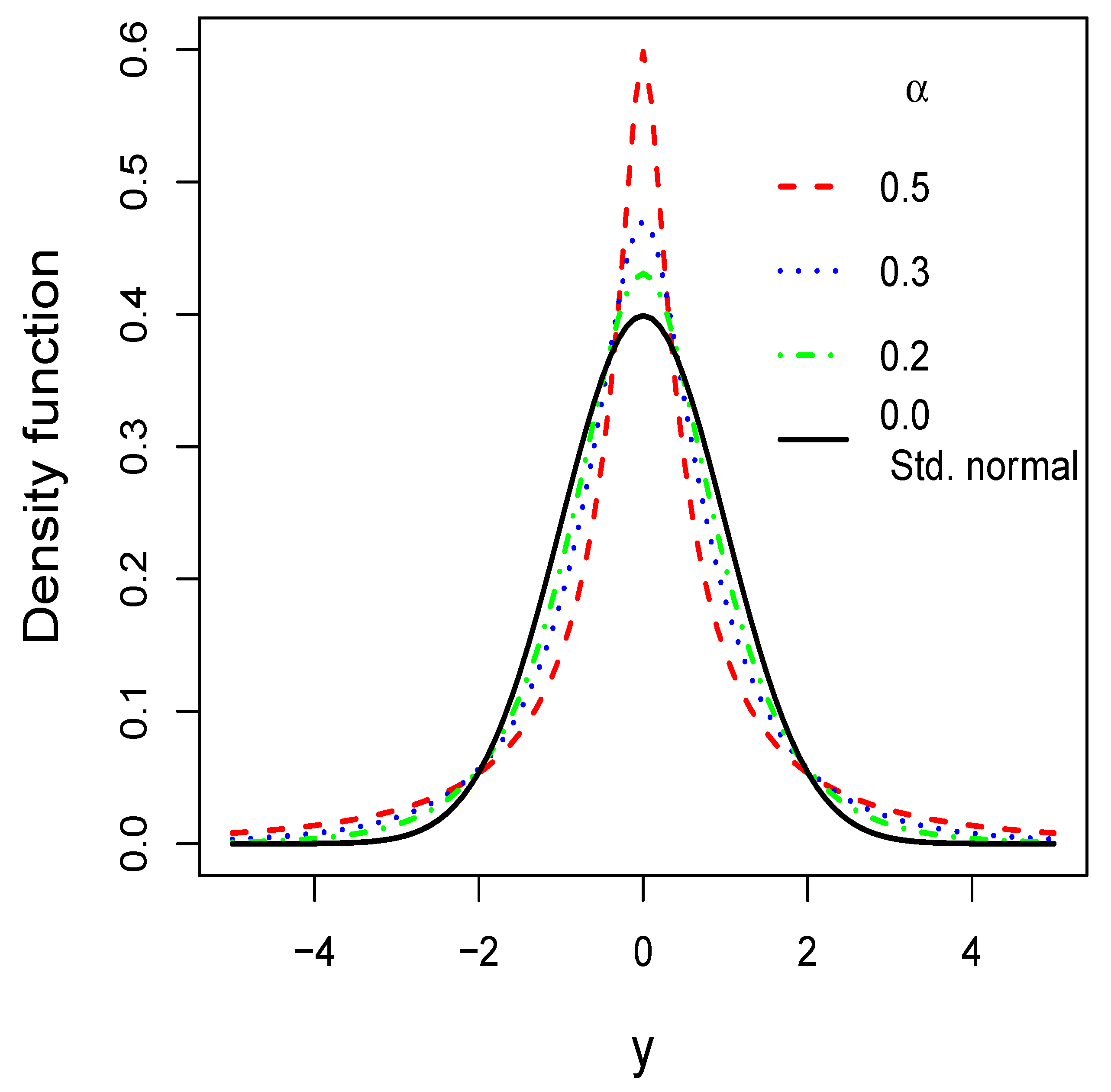
The slash distribution has a symmetrical bell shape similar to the normal, but with the distinctive feature of having heavier tails. As a consequence, the slash distribution may perform better when modeling data that exhibits high kurtosis levels. Specifically, the random variable
X follows the slash distribution with kurtosis parameter
, denoted as
, if it is represented as
where
and
are independent.
From Equation (
1), it can be verified that
as
, that is, the standard normal distribution is a limit case of the slash distribution. If
, then
X follows the canonic slash distribution proposed by Rogers and Tukey [
1].
The literature referring to slash distribution is extensive. Several properties and extensions of this distribution can be found in Mosteller and Tukey [
2], Johnson et al. [
3], Kafadar [
4], Wang and Genton [
5], Gómez et al. [
6], Arslan [
7], Genç [
8], Arslan and Genç [
9], and Genç [
10], among others.
In recent years, some authors have invested significant effort in developing studies focused on proposing distributions with even heavier tails than the slash distribution, which are originated by modifying the distribution of the denominator of Equation (
1). For example, Reyes et al. [
11] introduced the modified-slash distribution by considering that
U—in Equation (
1)—has the exponential distribution with mean 1/2. The authors illustrate that the modified-slash distribution—presenting the same parameter dimension as the slash distribution—can present a better performance in fitting data that exhibit a high kurtosis level. Similarly, Rojas et al. [
12] introduced the extended-slash distribution by replacing
by
W in Equation (
1), where
W has a beta distribution with mean
and variance
, with
. Here, the authors show that the extended-slash distribution—by presenting two kurtosis parameters—can perform better than the slash distribution when fitting high kurtosis data. In this same line, Reyes et al. [
13] proposed the generalized modified-slash distribution by replacing
by
W in Equation (
1), where
W has a gamma distribution with mean 2 and variance
, with
. Here, the authors show that the generalized modified-slash distribution can perform better than the slash and modified-slash distributions in fitting high kurtosis data.
The aim of this paper is to improve the modelling of high kurtosis data by introducing a new heavy-tailed modification of the slash distribution. This modification has such heavy tails that it can outperform even the modified-slash, extended-slash, and generalized modified-slash distributions. To achieve this end, we introduce a type II modified-slash distribution by replacing
by
V in Equation (
1), where
V has a Birnbaum–Saunders distribution.
The Birnbaum–Saunders distribution [
14,
15], originally derived to model the time to failure due to material fatigue, has played an important role in reliability studies. An important number of studies on properties, applications, and generalizations of this distribution can be found in the literature; see for example, Díaz-García and Leiva-Sánchez [
16], Sanhueza et al. [
17], and Gómez et al. [
18], to name a few.
Specifically, the random variable
V has a Birnbaum–Saunders distribution with a shape parameter
and scale parameter
, denoted as
, if it can, by being represented as
where
Z has a standard normal distribution.
The pdf of
V results to be
where
represents the pdf of standard normal distribution.
We provide evidence that by considering a Birnbaum–Saunders distribution—with representation and pdf given by Equations (
2) and (
3)—in the denominator of Equation (
1), a new extremely heavy-tailed distribution is defined, which can perform better than the slash, extended-slash, modified-slash, and generalized modified-slash distributions when fitting data that show high levels of kurtosis.
The remainder of this paper is summarized as follows. In
Section 2, we propose the new distribution and study some of its fundamental properties, such as stochastic representation, density, and raw moments.
Section 3 discusses the problem of parameter estimation via the moment and maximum likelihood methods. In addition, a simulation study is carried out to evaluate the behavior of the estimators. In
Section 4, two application examples aimed at evaluating the comparative performance of the proposed distribution are considered. Final comments are considered in
Section 5.
3. Parameter Estimation
Initially, this section discusses the parameter estimation for the T2MS distribution via the moment and maximum likelihood methods. Secondly, a simulation study is carried out in order to evaluate the behavior of the provided estimators.
3.1. Moment Estimation
Proposition 3. Let be an observed random sample for the random variable . Then, the moment estimators , , and for μ, σ, and α satisfy the following equations: where is the sample mean, is the sample variance, and is the sample Fisher’s kurtosis coefficient.
Proof. Equations (
8) and (
9) are direct consequences of equating the mean, variance, and Fisher’s kurtosis coefficient of the T2MS distribution—given in Corollaries 3 and 4—with the corresponding mean, variance, and Fisher’s kurtosis coefficient of the sample. □
3.2. Maximum Likelihood Estimation
Let
be an observed random sample of size
n on
. The log-likelihood function for
can be written as
where
and the components of the score vector
can be written as
where
Thus, the maximum likelihood estimator of can by obtained be solving the system of equations . However, it is not possible to obtain a closed form for , so the maximum likelihood estimates must be obtained by solving the system using numerical procedures.
Based on the approximation of the asymptotic variance of the maximum likelihood estimator, the interval estimation and the hypothesis tests for
,
, and
can be performed by computing the observed information matrix
. This matrix is given by
where
,
,
,
is as in Equation (
11), and the second partial derivatives are presented in
Appendix B.
So, the observed covariance matrix is the inverse of , , and the diagonal elements of are the variances of , , and , which we denote by , , and , respectively. Then, the asymptotic confidence intervals for , , and are , , and , respectively, where stands for the upper percentile of the standard normal distribution.
3.3. Practical Considerations
Regarding the parameter estimate via the moment method, we calculate the root of Equation (
8) using the rootSolve::uniroot.all( ) function [
21] in the R programming language. Once the estimate
is obtained, we use it to obtain the estimate
of
from the computation of Equation (
9).
Regarding the maximum likelihood estimation of the parameters of the T2MS
distribution, since the system of score equations does not lead to closed analytical expressions of the estimators, it is necessary to use a computational routine to obtain the root of this system. For this, we suggest the use of the rootSolve::multiroot( ) function [
21] in the R programming language. This function implements the Newton–Raphson method to obtain an approximation of the root of the system of nonlinear equations to be solved.
In this case, one may alternatively prefer to address the optimization problem
, subject to
,
and
, where
is as in Equation (
11). Here, we suggest using the stats::optim( ) function in the R programming language. In particular, we suggest the L-BFGS-B method [
22], which allows the parameter space to be specified by box constraints. We use the moment estimates discussed in
Section 3.1 as the values to initialize the iterative process.
The R codes used to obtain the estimates are provided in
Appendix A.2.
3.4. Simulation Study
In this section, we consider a simulation study aimed at evaluating the behavior of the moment and maximum likelihood estimators of the T2MS distribution parameters. We generate 1000 random samples from the T2MS distribution under scenarios A and B , and for each of the sample sizes n = 25, 50, 100, 200, and 400. The samples were generated considering the following steps, which were formulated from the stochastic representation of the T2MS random variable:
Choose values for , , , and n.
Generate .
Compute .
Generate .
Compute .
Repeat steps 2 to 5 n times.
For each generated sample, we calculate the M and ML estimates under the practical considerations of
Section 3.3.
Table 1 reports the average estimate and standard deviation for each 1000 moment and maximum likelihood estimates obtained in scenarios A and B, under the different sample sizes considered. In the table, the consistency property of the estimators provided by both estimation methods can be observed; note that as the sample size increases, the AEs obtained with both estimation methods approach the true values of the parameters and that the SDs decrease to zero. However, maximum likelihood estimators show greater efficiency and provide estimates with less bias; note that the bias associated with the maximum likelihood estimates is smaller (especially in small samples) and that the SDs are smaller.
4. Illustrations
In this section, we present two applications to real data that illustrate the usefulness of the type II modified slash (T2MS) distribution in fitting high kurtosis data. In each application, we compare the performance of the T2MS distribution with that of other heavy-tailed distributions, such as the slash (S), extended-slash (ES), modified-slash (MS), and generalized modified-slash (GMS) distributions. Below are the pdfs of these distributions:
- 1.
The S pdf;
where
,
is a location parameter,
is the scale parameter,
is a kurtosis parameter, and
is the pdf of the standard normal distribution.
- 2.
The ES pdf [
12];
where
,
is a location parameter,
is the scale parameter,
are kurtosis parameters, and
is the pdf of the standard normal distribution.
- 3.
The MS pdf [
11];
where
,
is a location parameter,
is the scale parameter, and
is a kurtosis parameter.
- 4.
The GMS pdf [
13];
where
,
is a location parameter,
is the scale parameter, and
is a kurtosis parameter.
In addition, we include the normal (N) distribution in the analysis because it is a limiting case of most of the aforementioned distributions.
In each application, we used the Anderson–Darling (AD) test to assess the quality of fit of the T2MS distribution. This test is computed using the goftest::ad.test( ) function [
23] of the R programming language. The comparative performance of the fitted distributions is evaluated using the Akaike Information Criterion (AIC) [
24] and the Bayesian Information Criterion (BIC) [
25].
4.1. Ant Movement Direction Data
In this section, we consider a set of observations on the initial direction of movement of 730 ants subjected to a visual stimulus. These data were originally presented in Jander [
26] and subsequently analyzed in Batschelet [
27], Sengupta and Pal [
28], and Jones and Pewsey [
29].
Figure 3 shows the boxplot of these data and
Table 2 shows the statistical summary. Here, it can be seen that the data present a very smooth level of negative skewness and a high level of kurtosis, explained by the presence of atypical observations. Taking these properties into account, we expect that the T2MS distribution can fit this dataset appropriately.
Table 3 reports the maximum likelihood estimates and the AIC and BIC values for the distributions fitted to the ants data. In this table, it is observed that the T2MS distribution has the lowest AIC and BIC values, suggesting that it should be selected for fitting the ant data. For the T2MS distribution, we obtain an observed statistic equal to 2.328 and a
p-value equal to 0.798 in the AD test, suggesting that this distribution performs well in fitting the data.
Figure 4 presents the histogram for the ants data and the pdfs fitted via the maximum likelihood method. In the figure, it can be seen that the pdf of the T2MS distribution is closest to the empirical frequencies both in the center and in the extremes of the histogram.
4.2. DEM/GBP Exchange Rate Returns Data
In this section, we consider a set of 1974 observations on the percentage returns of Deutsche mark/British pound (DEM/GBP) exchange rates from 1984 through 1991. This dataset can be found under the name MarkPound in the AER statistical package [
30] of the R programming language.
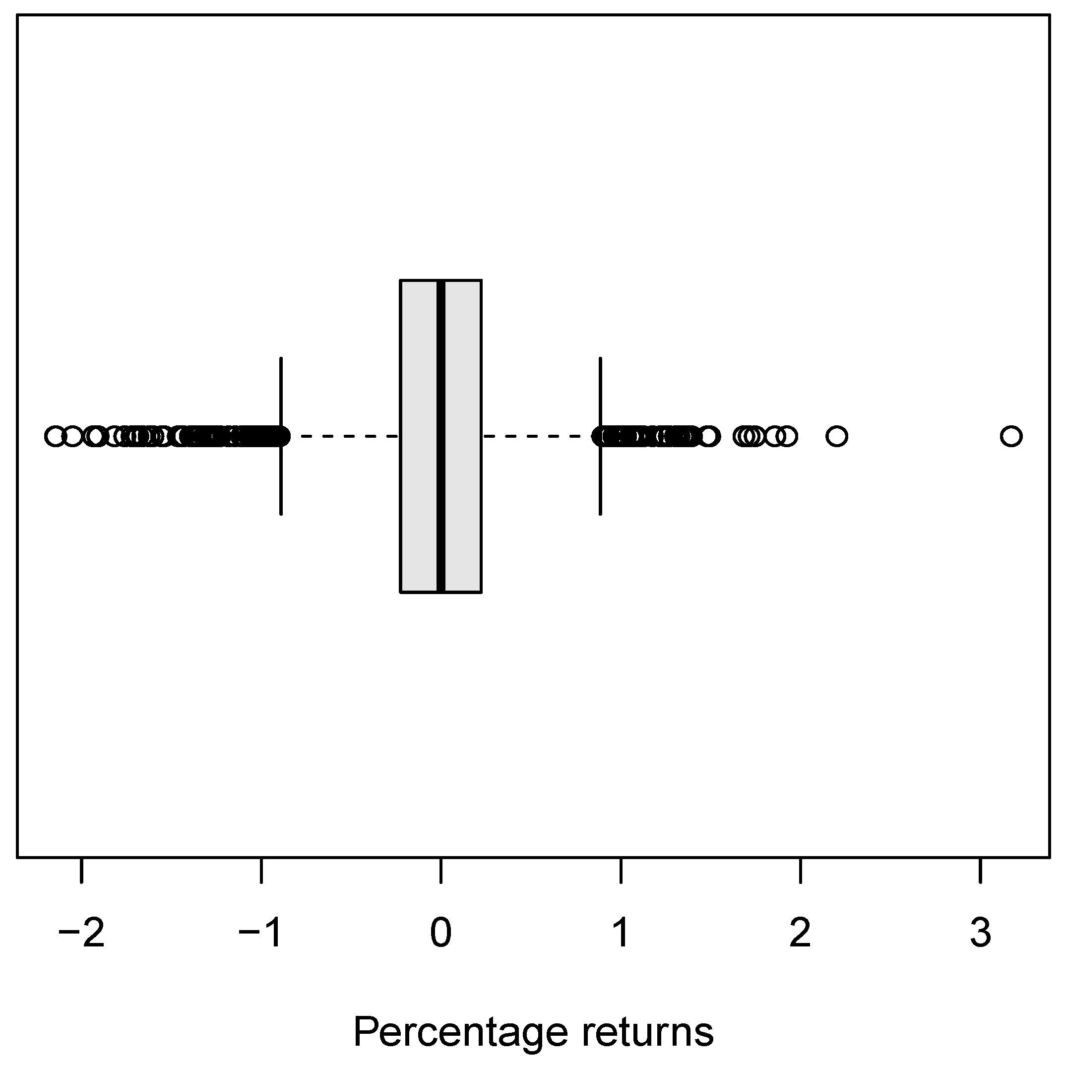
Table 4 shows some descriptive statistics for these data and
Figure 5 presents the boxplot. From these, it can be seen that the data present a smooth level of skewness and an important level of kurtosis explained by the presence of several atypical observations.
Table 5 reports the maximum likelihood estimates and the AIC and BIC values for the distributions fitted to the returns data. In this table, it is observed that the T2MS distribution has the lowest AIC and BIC values, suggesting that it should be selected for fitting the returns data. For the T2MS distribution, we obtain an observed statistic equal to 3.169 and a
p-value equal to 0.635 in the AD test, suggesting that this distribution performs well in fitting the data.
Figure 6 presents the histogram for the returns data and the pdfs fitted via the ML method. In the figure, it can be seen that the pdf of the T2MS distribution is closest to the empirical frequencies both in the center and in the extremes of the histogram.
5. Final Comments
In this article, we propose an alternative distribution for modeling high kurtosis data. The new distribution can be understood as a modified version of the slash distribution that —like other slash distributions in the literature—arises as a quotient of independent random variables. The novelty here is to consider a random variable with a Birnbaum–Saunders distribution in the denominator, something that we believe has not been previously explored. We observe that this modification of the representation of a slash random variable leads to a new distribution with extremely heavy tails, which can outperform other distributions in the analysis of high kurtosis data.
The fundamental properties of the new distribution are derived, among them the stochastic representation, the density function, and the raw moments with associated measures. Parameters in the proposed distribution are estimated using the moment and maximum likelihood methods. Through Monte Carlo simulation experiments, it is observed that both estimation methods provide consistent estimators. However, it could be observed that the maximum likelihood estimators are more efficient. Two applications to real data are considered. In each application, it is illustrated that the proposed distribution performs well in modeling high kurtosis data, even better than other heavy-tailed distributions in the literature.


