Contextual Augmentation Based on Metric-Guided Features for Ocular Axial Length Prediction

Abstract

Ocular axial length (AL) measurement is important in ophthalmology because it should be considered prior to operations, such as strabismus surgery or cataract surgery, and the automation of AL measurement with easily obtained retinal fundus images has been studied. However, the performance of deep learning methods inevitably depends on distribution of the data set used, and the lack of data is an issue that needs to be addressed. In this study, we propose a framework for generating pairs of fundus images and their corresponding ALs to improve the AL inference. The generator’s encoder was trained independently using metric learning based on the AL information. A random vector and zero padding were incorporated into the generator to increase data creation flexibility, after which AL information was inserted as conditional information. We verified the effectiveness of this framework by evaluating the performance of AL inference models after training them on a combined data set comprising privately collected actual data and data generated by the proposed method. Compared to using only the actual data set, the mean absolute error and standard deviation of the proposed method decreased from 10.23 and 2.56 to 3.96 and 0.23, respectively, even with a smaller number of layers in the AL prediction models.

1. Introduction

As a subtype of artificial intelligence (AI), deep learning is a method inspired by the neural architecture inside the human brain that has significantly reduced bottlenecks in various fields owing to recent developments in computer power [1,2]. Deep learning is actively applied in ophthalmology, and its main applications include retinal image analysis, retinal disease classification, and retinal pathology identification [3,4,5,6]. Retinal image analysis involves detecting and segmenting biological components in retinal images or screening high-quality images. Fundus images, one of the most commonly used images in ophthalmology, show the retinal vessels, optic disc, and fovea; rapid and accurate identification of these components is important for achieving diagnosis automation and downstream tasks [7,8]. In addition, retinal disease classification and retinal pathology segmentation have attracted significant research attention for automating retinopathy diagnoses [9,10].

Beyond classification, researchers have recently attempted to apply deep learning to regression tasks. For example, the retinal nerve fiber layer thickness (RNFL) and the minimum rim width at the Bruch’s membrane opening on the spectral-domain optical coherence tomography scale were predicted to aid the automatic diagnosis of glaucoma [11]. As another example of a regression task, axial length (AL) is measured by optical biometry, which requires sophisticated skills and large spaces [12]. In addition, the prediction of ocular AL, defined as the distance between the anterior surface of the cornea and the retinal pigment epithelium based on a fundus image using a deep learning method, has been studied [13,14].

AL is considered as one of the important biometrics in ophthalmology because it is used as a parameter for making intraocular lenses before cataract surgery [15] and is related to the development of eye diseases such as glaucoma and myopic degeneration [16,17]. The linkage between AL and fundus image can be found in diverse ways. Retinal thinning in highly myopic eyes has been seen in the peripheral areas, whereas it is not observed in the fovea [18]. It is also known that maculopathies such as myopic macular degeneration and macular diseases are associated directly or indirectly with AL [19,20].

As with other fields, ophthalmological deep learning applications need as much useful data as possible to improve generalization abilities and avoid model overfitting. Therefore, in addition to the available data, it is necessary to artificially create data to compensate for the insufficient data distribution. A simpler approach for generating data is low-level image processing, such as rotating, clipping, and flipping existing data or random noisy injection [21,22]. Another strategy involves learning data distribution by training a neural network with existing data and generating it through an architecture [23,24]. If supportive information can help a neural network learn data distribution, corresponding variations can be applied [25,26].

In this study, we propose a method for generating valid data, enriching the diversity of training data, and improving the performance of the downstream prediction network. A notable feature of this study is the characteristics of the data and the method of generation. The data to be generated are fundus images and corresponding ALs, where AL is a continuous real value and not a discrete value. The approach to generating this pair of data has not been extensively investigated because it is not as simple as the usual image generation methods that deal with images bound to the target of discrete values, such as class. First, continuous real AL values must be divided into fixed intervals. For generation, a generating network considers only the corresponding fundus images in one AL range as the target and images in another AL range as the input. In this manner, insufficient data can be generated using the data in the part with high frequency in the data distribution, which also provides continuity between images in different AL ranges. Images in the neighboring range were used for generation to gain confidence in the validity of the generated images, which was demonstrated by the improvement in the performance of the downstream AL prediction, as illustrated in Figure 1.

Feature alignment is a strategy for establishing a relationship between two different feature domains or between features and other relevant information. If fundus images are fed into the encoder (Figure 1) in the training phase without any reference information, it is difficult to obtain a clear relationship between the latent features of the images and the corresponding ALs. This unconvincing latent feature vector negatively affects the decoders when generating effective images, as demonstrated by the experiment. The feature alignment is implemented by corresponding the metric of the distances of AL with the metric of the element-wise distances of the latent feature vector and grouping with zero padding for the region representation after encoding.

In summary, our main contributions are featured in the following aspects:

• The proposed framework confirms that the pairs of generated fundus images and AL can contribute to a reduction in the variance and bias of the prediction model, indicating that the generated pairs can provide regularization effects on the prediction networks.
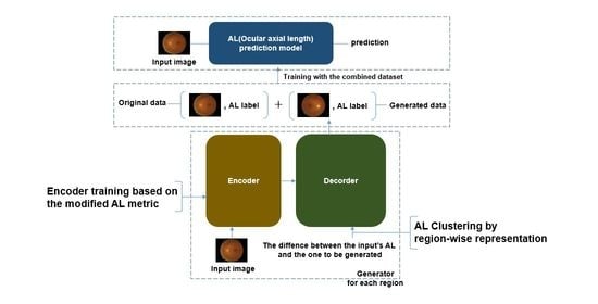
• The independent training of the encoder in the proposed metric-based method and grouping of the latent feature vectors after the encoder are effective for generating valid data.
• Using the data set generated by the proposed method, improved AL prediction results can be obtained using the prediction models, even with fewer weights.

The rest of this paper is organized as follows: Section 2 reviews the works related to this study. Section 3 describes the proposed data augmentation method. In Section 4, the experiments and results of the proposed method are explained. A discussion is provided in Section 5, with the conclusions presented in Section 6.

2. Related Work

In this section, related studies from three aspects are briefly reviewed.

2.1. Medical Image Synthesis

Recent advances in medical image synthesis have been achieved through deep learning, owing to its decomposition and reconstruction capabilities. Most studies use deep learning architectures in the medical field, including U-Net-based and generative adversarial network (GAN)-based architectures [27,28]. Medical image synthesis aims to restore poor-quality images or convert them into new images in a similar domain [24]. A previous study modified a U-Net-based architecture, enabling it to possess three-dimensional convolutional layers for generating positron (PET) images [29]. Another study replaced the pooling layer of U-Net for downsampling with a convolution layer to generate improved-quality computed tomography images [30]. Furthermore, the positive effect of creating local skip connections to preserve details in the U-Net architecture when reconstructing sparsely sampled MRIs was experimentally demonstrated [31].

A previous study proposed a framework with two distinct GANs to generate DR images [32]. The first GAN was responsible for image conversion between the source and target domains, whereas the second GAN generated DR images using the conditional information of the severity class and structural and lesion masks. In addition, CycleGAN was implemented for domain translation, with multiscale inputs enabled for the second GAN. Another study developed a cycle-consistent GAN by modifying the loss function by introducing a mean absolute difference that counts the number of incorrectly generated pixels and the gradient descent loss between the target and source PET images [33]. For MRI generation, a previous study adopted the ResNet architecture in the generator to preserve detailed signals, with the ratio between the l₁ and l₂ costs used as the loss function to remove noise while maintaining the fine texture of the images [34].

This study adopted U-Net as the basic architectural structure for several reasons, including proving the novelty of this method. For a GAN, the generator and discriminator should be trained simultaneously without mode collapse, making it difficult to insert the continuous value of conditional information (AL) and determine its effectiveness.

2.2. Augmentation

Studies have been conducted in several fields to improve downstream tasks via augmentation by generating training samples: In one study [35], the impact of data augmentation was assessed using simple geometric operations under various conditions, including binary and multilevel classifications in leukemia diagnosis tasks. An augmentation method for generating functional magnetic resonance (fMRI) images that minimizes the problems of feature and distribution mismatches while preserving the sparse reconstruction relation over the entire data set of the input space was developed [36]. Arterial spin labeling (ASL) images were synthesized to provide useful data based on well-established image-based dementia data sets to improve the performance of dementia disease diagnosis [37]. A locally constrained GAN-based ensemble was designed by adopting an attention-based feature pyramid model to synthesize ASL images. The concept of negative transfer and structural consistency to optimize the modified GAN builds augmented domains based on data in the source domain and color channel shuffling [38]. The effectiveness and robustness of this method were demonstrated using a person re-identification (ReID) task.

2.3. Metric Learning

Metric learning is an important deep learning technique that uses measurable information to help a neural network better discriminate between input vectors. Measurable information depends on the tasks handled by a neural network, which can introduce useful metrics for making the input data distinguishable. Among various studies, a pseudo-labeling framework for addressing class imbalance was designed [39]. The neural network that forms the framework was trained using the loss function, which calculates the square distances of the embedded vectors of the input data. The introduced margin value forced the vectors of the same classes to be clustered, whereas the vectors of the different classes were separated. The contrastive loss function was used to determine whether the two input patch data sets belonged to the same class [40]. Furthermore, the embedded feature vectors obtained by neural networks trained by metric learning can be clustered in an unsupervised manner. Metric learning was applied to multiclass classification using triplet loss by introducing a generalized version of multiclass N-pair loss [41]. In addition to the variation in Euclidean distance, the chi-squared value was used as measurable information; furthermore, a modified triplet loss function that incorporates the chi-squared distances between the histogram vectors of the features was designed [42].

3. Method

In this section, structures of neural networks with a loss function for training are introduced, followed by a data augmentation strategy.

3.1. Neural Networks

In this study, we developed an AL prediction framework comprising the following three parts: generator, data combination, and AL predictor. The generator created paired data of fundus images and the corresponding ALs in the infrequent regions of the AL distribution in Figure 2, while the AL prediction models were devised to evaluate the validity of the generated data set.

3.1.1. Generator

The generator generates images and the corresponding ALs based on the original pairs located near them in the data distribution. The generator architecture is based on a U-Net shape in which the input and output have the same dimensions. The advantage of adopting the U-Net architecture is its ability to flexibly fuse the coarse information of global abstracts with the fine information of local details through skip connections. The proposed network exhibited four hierarchical representations, with each semantic piece of information reserved and reused at the same level of decoding path. The generator mainly comprises an encoder, a middle part for producing and condensing the feature representation with AL conditional information, and a decoder for generating images based on the feature vector.

• Encoder

The encoder, i.e., the front part of the generator, converts the input images into condensed representations. As shown in Figure 3b, its structure is composed of five convolutional layers in a row, with the last fully connected layer. The convolution layers contains 3 × 3 kernels with two strides, and the fully connected layer contains 16 nodes.

For training, we used metric learning that reflects the Euclidean distance of the AL to the distance of the feature vectors. The fundus images in the same AL distribution region were fed into two different encoders with the same weights; this separate feedforward enabled the evaluation of the relationship between the corresponding ALs while updating the shared weights.

$$\stackrel{⃑}{D_f}=\left|f_{enc}\left(X_1\right)-f_{enc}\left(X_2\right)\right|$$

(1)

$$\stackrel{⃑}{D_{AL}}=\left|A{L}_{X_1}-A{L}_{X_2}\right|1_{\stackrel{⃑}{D_f}}$$

(2)

$\mathrm{w}\mathrm{h}\mathrm{e}\mathrm{r}\mathrm{e}A{L}_{X_1},A{L}_{X_2}\in R_{AL},\mathrm{a}\mathrm{n}\mathrm{d}{1}_{\stackrel{⃑}{D_f}}\mathrm{i}\mathrm{s}\mathrm{a}\mathrm{l}\mathrm{l}—\mathrm{o}\mathrm{n}\mathrm{e}\mathrm{s}\mathrm{v}\mathrm{e}\mathrm{c}\mathrm{t}\mathrm{o}\mathrm{r}\mathrm{w}\mathrm{i}\mathrm{t}\mathrm{h}\mathrm{t}\mathrm{h}\mathrm{e}\mathrm{s}\mathrm{a}\mathrm{m}\mathrm{e}\mathrm{d}\mathrm{i}\mathrm{m}\mathrm{e}\mathrm{n}\mathrm{s}\mathrm{i}\mathrm{o}\mathrm{n}\mathrm{a}\mathrm{s}\stackrel{⃑}{D_f}.$

$$L_{mean}=\left|\stackrel{⃑}{D_{f_{mean}}}-a\cdot {\stackrel{⃑}{D_{AL}}}^b\right|$$

(3)

$$L_{var}=|\stackrel{⃑}{D_{f_{var}}}-c\cdot {\stackrel{⃑}{D_{AL}}}^d|$$

(4)

$$L_{enc}=L_{mean}+L_{var}$$

(5)

$D_f\mathrm{a}\mathrm{n}\mathrm{d}{D}_{AL}$ in (1) and (2) are the Euclidean distances between the feature vectors of two given input images, $X_1\mathrm{a}\mathrm{n}\mathrm{d}{X}_2$, associated with the corresponding ALs, $A{L}_{X_1}\mathrm{a}\mathrm{n}\mathrm{d}A{L}_{X_2}$, respectively, where $A{L}_{X_1}\mathrm{a}\mathrm{n}\mathrm{d}A{L}_{X_2}$ are the elements in a specific region, $R_{AL}$. As illustrated in (3) and (4), the encoder must be trained to minimize the difference between the distances between the ALs and each component of the encoded vectors. Note that the distance in the feature space does not follow the metric in the Euclidean distance because the feature space, which is set by the encoder, is not a Euclidean space. Therefore, additional hyperparameters, i.e., a, b, c, and d, were introduced to match both distances, thereby reducing the distance error as much as possible. The feature distance increases or decreases linearly by manipulating a and b, using the power to manipulate c and d.

The output vector of the encoder is a 16-dimensional vector divided into the mean vector, $D_{f_{mean}}$, and variance vector, $D_{f_{var}}$. The first eight feature components were defined as $D_{f_{mean}}$, whereas the remaining eight components were defined as $D_{f_{var}}$. These vectors were used to calculate the intermediate results of the feature vector modification according to (6) in the middle of the generator.

• Feature vector modification

After the input images were encoded using the encoder, the output feature vector was 16-dimensional and divided into mean and variance vectors with eight dimensions. As illustrated in (6), the mean vector can be considered the central point of the corresponding input image, whereas the variance vector can be considered the amount of deviation of the encoded vector from the central point. In this manner, the feature component was integrated by fixing the first eight feature components and flexibly choosing the remaining eight.

In this setting, the variance can be controlled by adopting a random vector in the random distribution with the range [0, 1] to ensure different images can be generated flexibly for downstream AL inference. In this study, the random vector is produced with a uniform distribution because if the probabilities are uniform, various vectors around the mean vector can be chosen without exceeding the radius of the variance vector.

$$f=f_{enc}(X{)}_{mean}+f_{enc}(X{)}_{var}\odot u,u~U(0,1)$$

(6)

$$A{L}_{diff}=A{L}_{X_2}-A{L}_{X_1}$$

(7)

$$f^{\mathrm{″}}=Concatenate(f^{\mathrm{\prime }},A{L}_{diff})$$

(8)

Equation (6) is a mathematical description of the process, where $f,X,\mathrm{a}\mathrm{n}\mathrm{d}u$ are the adaptive feature vector, input image, and random vector, respectively. As the created random vectors with equal probabilities can produce varying f in the region centered in the mean vector and with the radius of the variance vector, a uniform distribution is used to create the random vector to provide the generators with flexibility for image generation.

After evaluating the adaptive feature vector, the AL difference, $A{L}_{diff}$, should be added in (7). As this information was used to generate images using the decoder, the AL difference was obtained by subtracting the input AL from the AL to be generated.

• Feature vector grouping

The last piece of information is the zero elements for the spatial separation of the regions. As listed in

Table 1. Region Representation $f\prime$.

Region (mm)	$\mathit{f}\prime$	Region (mm)	$\mathit{f}\prime$
20.5–21.0	[$f$,$f$,0,0,0,0,0,0,0,0]	30.0–30.5	[$f$,0,0,0,0,0,0,0,0,$f$]
21.0–21.5	[$f$,0,$f$,0,0,0,0,0,0,0]	30.5–31.0	[0,$f$,$f$,0,0,0,0,0,0,0]
21.5–22.0	[$f$,0,0,$f$,0,0,0,0,0,0]	31.0–31.5	[0,$f$,0,$f$,0,0,0,0,0,0]
27.5–28.0	[$f$,0,0,0,$f$,0,0,0,0,0]	31.5–32.0	[0,$f$,0,0,$f$,0,0,0,0,0]
28.0–28.5	[$f$,0,0,0,0,$f$,0,0,0,0]	32.0–32.5	[0,$f$,0,0,0,$f$,0,0,0,0]
28.5–29.0	[$f$,0,0,0,0,0,$f$,0,0,0]	32.5–33.0	[0,$f$,0,0,0,0,$f$,0,0,0]
29.0–29.5	[$f$,0,0,0,0,0,0,$f$,0,0]	33.0–33.5	[0,$f$,0,0,0,0,0,$f$,0,0]
29.5–30.0	[$f$,0,0,0,0,0,0,0,$f$,0]	34.5–35.0	[0,$f$,0,0,0,0,0,0,$f$,0]

, each AL region exhibits its own form of representation, $f^{\mathrm{\prime }}$, with the adaptive feature vectors in distinct quadrants. The final feature vector modification, represented as $f^{\mathrm{″}}$ in (8), was performed by concatenating the region representation, $f^{\mathrm{\prime }}$, with the AL difference, ${AL}_{diff}$. In summary, the modified feature vector includes information on the AL region with space separation and the AL difference between the target AL and the input AL by adding another axis for this scalar value.

Figure 4 shows a diagram of the feature vector modification in the middle of the generator. According to (3) and (4), the encoder is trained such that the mean and variance vector points are at a maximum distance from each other as $\mathrm{a}\cdot |{\mathrm{R}}_{\mathrm{A}\mathrm{L}}{|}^{\mathrm{b}}$ and $\mathrm{c}\cdot |{\mathrm{R}}_{\mathrm{A}\mathrm{L}}{|}^{\mathrm{d}}$, respectively, where $\left|R_{AL}\right|$ is the interval of the AL region, which is 0.5 mm in this study. The advantages of the two modification steps include the following: (i) encoded points can be crowded with a finite distance that reflects the real distance between axial lengths, (ii) specified AL region information, as well as the AL to be generated, are present in the modified feature vector, and (iii) possibility of generated images overlapping with different AL can be reduced.

• Decoder

The special feature of the decoder of the U-net is its ability to share the encoder’s hierarchical results by concatenating them with the results in the corresponding levels through the decoder path. These bifurcations help to efficiently update the weights of both paths by referencing the modified feature vectors in the middle and also compensate for the inevitable information loss through the encoder path because of the restricted receptive fields of the convolution processes.

The decoder path begins with a modified feature vector of 24 dimensions and is subsequently fed into the next fully connected layer via reshaping to exhibit 4 × 4 × 4 feature maps of the same size as the last level of the encoder path. Thereafter, four transposed convolution processes are conducted to increase the dimensions until the final outputs exhibit the same size as the input images. Leaky ReLU and batch normalization layers were used as nonlinear activations for each level. In addition, the height and width of each feature map were designed to match the size of the feature map at that level in the encoder path for concatenation, as shown in Figure 3a. The channel size was doubled from 4 to 32, and the final output channel was 3, representing the three-color channels.

3.1.2. AL Predictor

As shown in Figure 3c, The AL predictor was a ResNet consisting of consecutive residual blocks for feature extraction, and fully connected layers for the regression. The residual blocks exhibit shortcut connections that can preserve the detailed information from the previous layer and prevent explosion and vanishing of gradients during training [43]. The path for the extraction of features in each residual block utilized two convolutional layers with batch normalization and ReLU activation. The number of channels of the convolutional layers of the residual blocks doubled at 64, and the kernel size was 3 × 3 which produced the same height and width of the inputs. The 2 and 4 residual blocks were used for base model and deeper model, respectively. Lastly, the number of nodes for the fully connected layers were 50 and 1, and the last one represents the predicted value.

3.2. The Procedure of the Data Augmentation

As described in Algorithm 1, the overall procedure can be divided into six major steps. Before the first step, the data set needs to be separated according to a certain length of AL interval, and a generator should be created and trained for each region. For the first step for a region, the encoder embedded in the generator is trained with the images and AL in the corresponding regions. The encoders for all the regions are trained using the proposed metric learning method as input images can be mapped into its modified AL metric that fits for the hidden space, represented by (1)–(5). The second step is training the generators for the total regions. After embedding the trained weights in the encoder into the corresponding generators, the random vector and AL difference were utilized to produce the modified feature vector as (6)–(7). During training, the region of the input images needs to be the previous or the next region that the label images belong to, because referencing the data in the nearest region is assumed to be more efficient in terms of generating the data. The third step involves the generation of the data for all regions, and the number of the data combined with the existing data for each region are set. The fourth step is training the AL predictor with the mean absolute error loss function, and, finally, the AL is inferenced. In Algorithm 1, L_enc is the loss function for training the encoders as represented in (5) and L_gen is the mean absolute error (MAE) loss function for training the generator.

Algorithm 1: Pseudo-code for the method.

Input:

Pairs for training encoder: (xenc,i, yenc,i) i = 1, 2 in the same region

Pairs for training generator: (xgen, ygen), (xgen,label, ygen,label) in different regions

Pairs for training AL prediction models: (xpred, ylabel)

Images for inference: xinf

Hyper-parameters for encoder

Output:

Predicted AL: O

Step 0: Dividing the data set according to a certain length of AL interval

Create an encoder and a generator for each region

Step 1: Training encoder for each region

Initialize weights of encoder

Set the hyperparameters for encoder

For the iteration number for the encoder do

Compute Enc1 = encoder(xenc,1) and

Enc2 = encoder(xenc,2)

Compute Lenc = Lenc(Enc1, Enc2, yenc,1, yenc,2)

Compute gradient genc = $\nabla$Lenc

Update weights wenc = SGD(genc)

End for

Save wenc

Step 2: Training the generator for each region

Initialize wgen

Replace the encoder weights with wenc in Step 1

Stop updating the weights of the encoder

For the iteration number for the generator do

Compute Enc = encoder(xgen) in Generator

Create a random vector r

Compute ALdiff = ygen,1 − ygen,2

Feature vector modification: Compute f″ with Enc, r, and ALdiff

Feature vector grouping according to Table 1

Compute = Decoder(f″)

Compute Loss Lgen = MAE(xgenerated, xlabel)

Compute gradient ggen = $\nabla$Lgen

Update weights wgen = SGD(ggen)

End for

Save wgen

Step 3: Image combining

Set the number of images needed for each region

Calculate the number of generated images needed for each region

Generate the images and ALs with the generators

Combine the generated data sets with the original data set

Step 4: Training AL prediction models

Initialize wpred

For the iteration number for AL prediction models do

Compute results ypredicted = AL prediction models(xinf)

Compute Loss Lpred = MAE(ypredicted, ylabel)

Compute gradient gpred = $\nabla$Lpred

Update weights wpred = ADAM(gpred)

End For

Step 5: AL inference

Compute O = AL prediction model(xinf)

4. Experiment

4.1. Data Set

A total of 1895 fundus images were collected using a Topcon fundus camera (Triton, software version 10.10; Topcon Corp., Tokyo, Japan). The data set was privately gathered retrospectively from ophthalmological examinations of patients at the university medical center, with 599 images manually excluded by ophthalmologists as they did not contain enough information about the fundus status, while the remaining 1296 images were used in this study. Corresponding AL data were obtained by averaging five values measured by the experts using IOL Master version 5.4 (Carl Zeiss Meditec AG, Jena, Germany). This study adhered to the tenets of the Declaration of Helsinki and was approved by the Institutional Review Board of Korea University Anam Hospital, No. 2019AN0314 (date of approval: 15 July 2019). The ALs included those of normal, hyperopic, and myopic eyes, ranging from 22 to 35 mm. Poor images of biolandmarks with low visibility, such as retinal vessels, optic discs, and fovea, were excluded by ophthalmology experts from the university hospital. As shown in the distribution of AL in Figure 2, 50% of the data were concentrated in the range of 23–25 mm, and the frequency decreased abruptly as the AL deviated from this region.

4.2. Experimental Setup

The framework can be divided into two main components: data generation and AL prediction. To generate data, the encoder in the generator can be separately trained using the proposed method, and the two AL prediction models can be trained using the existing and generated data. In this study, the networks were implemented using an Intel(R) Xeon(R) CPU E5-2620, with a clock speed of 2.10 GHz, 64 GB of memory, and four RTX 2080Ti GPUs. The AL prediction models were trained using the adaptive moment estimation (Adam) optimization method, and the generators and encoders were trained using stochastic gradient descent (SGD) to update the weights. The Adam optimization method was chosen because of its ability to adapt the learning rate based on the local shape of the manifold, which helps the networks find the minimum of the loss function [44]. SGD was chosen because learning the general expression of fundus images is important for generators [45,46]. The AL prediction models were trained using the Adam optimization method, and the generators were trained using SGD to update the weights. Five batches were prepared; the number of iterations for the encoder, generator, and AL predictor was 1000, 10,000, and 2000, respectively.

The fundus images were cropped to 128 × 128 pixels, with the regression results evaluated using mean absolute error (MAE) and standard deviation (std), and the unit for MAE was mm for the consistency with the unit for AL. Experimental performance was assessed by randomly selecting 100 pairs according to the regions, with half in the 22~27.5 mm region, where the majority of the data were located in the distribution, and the remaining half in the other region (i.e., 20–22 mm and 27.5–35 mm). This selection was performed to prevent an unreliable assessment, followed by biased test data obtained from the most crowded region. The hyper-parameter tuning was conducted with the randomized search in greedy approach. The learning rates of each model were chosen after trial with some representative values such as powers of the 0.1 for the generators and AL prediction models, and the values of 0.001 were selected to be the best. The values for the hyper-parameters in the proposed loss function for the encoders, a, b, c, and d in (3) and (4), were assigned step by step. The a, b for the mean vector loss in (3) were decided first and then the other two for the variance vector loss in (4) were decided. The specific values for those hyper-parameters were shown in the results sections. Lastly, the total number of data sets for each region for training was set to be 30 including the existing data set and the newly generated data set, heuristically.

Experiments

• Experiments on the effect of the different layer depth of the AL predictor

The layer depth is one of the basic parameters that affects the performance of a neural network. Furthermore, in terms of the utilization of the generated data, the performances of same networks with different layer depth indicates its validity and effectiveness, because a large data set provides room to reduce the depth of the network. Therefore, we designed two ResNet models as the AL prediction models to not only compare the performances of the two networks but also verify whether the data were well generated. As shown in Figure 3c, the deeper model contains four residual blocks, whereas the base model contains two residual blocks. In addition, the architecture of the residual block and the fully connected layers, and the other parts of the networks, are the same.

• Experiments on the feature vector modification

The architecture of the generator was designed based on the form of U-Net architecture. However, the proposed architecture was improved to enable the generation of pairs of the fundus images and the corresponding ALs. As previously discussed, the random vectors were utilized to provide the variation for the generation [47], and the AL difference between the input AL and output AL was inserted into the modified feature vector to match the output image. Furthermore, as shown in the Table 1, the modified feature components were arranged such that they were located in the separate quadrants employing the zero padding. The 16 generators for the 16 regions were created, and each model was trained twice with and without this space separation. The effectiveness of the feature vector modification was verified by comparing the performances of the AL prediction models trained using the generated data with the two options.

• Experiments on the independently trained encoder

The encoder in the generator converts a point in the image space into the corresponding point in the feature space. Two methods were employed to train the encoder. First, the encoder for each region was trained dependently via the end-to-end training of the generator. The other method involved the independent training of the encoder with the specified metric function of mapping the fundus images into the ALs as represented in (1)–(5). Compared to the former method, the latter offers the flexibility in the generator design and interpretability of the architecture. The effectiveness of the independent training method was verified by testing the generated images produced by the generators with these options. This section may be divided by subheadings. It should provide a concise and precise description of the experimental results, their interpretation, as well as the experimental conclusions that can be drawn.

4.3. Result

This section presents a systematic analysis of the performance of the proposed framework. First, the generated pairs of fundus images and ALs are shown, along with a description of the focus of the generators during image generation. Second, to provide a criterion for verifying the effectiveness of the main performance results, the baseline performances are evaluated using two AL prediction models trained only on the actual training data set. The last three results are the assessment results of the two AL prediction models trained on the data set that combined the actual data set and the data sets generated with the three different options, as described in the following subsections. Except for the analysis of the generated pairs, all performances are evaluated using the same carefully selected test data set and metrics (i.e., MAE and std).

• Results of the generated pairs

Two main characteristics were observed in the generated images: partial preservation of the biological landmarks and dependency on the reference data. For a visual representation, the samples in the specified regions are shown in Figure 5, which shows three actual images in the first column as reference images and nine generated images in the other columns. The top row in Figure 5 shows a group of images whose ALs belong to the 21.0–21.5 mm region.

Compared with the actual image, some information on the biological landmarks was lost in the generated images. For example, the location of the fovea and contents inside the optic discs were not retained. However, the locations and edges of the optic discs and their neighboring areas tended to remain unchanged, and the edge of the optic cup inside the optic disc was also visible. In addition, the retinal vessels in the generated images were vaguely expressed, while the small branches tended to disappear. Furthermore, as shown in the second row of the Figure 5, when the actual fundus images had the diseased areas of the retinal detachment, the areas were not generated. Despite these representation losses, other information, such as the overall structure of the background and its color variation, was reproduced. Through these observations, it was confirmed that some details of the biological landmarks in the fundus images could not be considered important for inferring AL, whereas some information which was located on the background structure and areas nearby the edges of the landmarks appeared to be crucial.

Images whose ALs belong to the 30.5–31.0 and 31.0–31.5 mm regions are shown in the second and third rows in Figure 5, respectively. The overall background patterns of the generated images of the 30.5–31.0 mm region were reproduced. However, biological landmarks were absent in all the generated images in these cases and tended to contain only the colors and shape of the optic disc, indicating that the generator could only focus on shaping the low frequencies of the data. This may be attributed to the lack of data, which resulted in the poor learning of those regions. At ALs above 30 mm, the number of data set decreased rapidly. For the data set used, the average number was 2.13 per interval and the maximum was 4. In case of samples in the 31.0–31.3 mm region in Figure 5, as the number of original data set in the region is 1, the generator can only generate the points near it, indicating that its similar images are always produced.

• Results of the baselines

The results presented in this subsection were obtained by averaging the metric values of the total 24 regions from 21–35 mm. The baseline result represents the score of how accurately the AL prediction models were trained on the actual data set. The results of deeper model indicate its superiority to base model (

Table 2. Performance of the two AL prediction models, the base model and deeper model, after training on the actual data.

AL Prediction Model	MAE	Std
Base model	10.23	2.56
Deeper model	5.49	1.43

). With an increase in the depth of the model, the MAE and std decreased from 10.23 and 2.56 to 5.49 and 1.43, respectively. The scatter plot revealed that the std of the corresponding region of deeper model was better than that of base model (Figure 6). This indicates that base model recorded both higher bias and variance, and the results came from the fact that the deeper model has more weights to gain regression power.

• Results of the Experiments on the feature grouping using end-to-end learning

The end-to-end learning is the one-time training of a model. In this constraint, the feature grouping in the middle of the architectures ensures the separation of the different generated points in the pair space. The effect of feature grouping is presented in

Table 3. Analysis of the effect of feature vector grouping using the end-to-end training of generator.

Use of Feature Vector Grouping	AL Prediction Model
	Base Model		Deeper Model
	MAE	Std	MAE	Std
No	8.32	6.92	5.32	1.21
Yes	4.29	0.43	4.38	0.97

, and it indicates that using the generated images with the feature grouping exhibited a positive effect on training both AL prediction models.

For base model, the MAE and std decreased from 8.32 and 6.92 to 4.29 and 0.43, respectively. The performance of deeper model also improved, and the MAE and std decreased from 5.32 and 1.21 to 4.38 and 0.97, respectively. This was further verified by the scatter plots from the feature grouping option in Figure 7, regardless of the depth of the AL predictors. The error values and their variances were also lower, meaning that the pairs generated using the feature grouping were closer to points of the actual pairs without compromising the generalization. In detail, the deeper model still had better prediction power than the other one, which means that more weights were still needed to analyze the fundus images, even though the generated data set had been helpful for possessing more information by the weights of the models.

• Results of the experiments on the independent training of the encoder

The encoders used in this experiment were separately trained in a way that the Euclidean distance between ALs is mapped into the distance between the encoded vectors in hidden metric of the feature space. By doing so, the encoder can learn the extra information about the hidden metric explicitly, which helps to generate data with better qualities. The values listed in Table 3 and

Table 4. Analysis of the effect of feature vector grouping and the independent training of the encoder.

Use of Feature Vector Grouping	Encoder		AL Prediction Model
	Hyper- Parameters (a:0.01 and b:1)		Base Model		Deeper Model
	c	d	MAE	Std	MAE	Std
No	5	2	5.79	1.52	6.49	2.06
	10	2	7.37	3.51	4.28	0.21
Yes	5	2	3.96	0.23	4.33	0.25
	10	2	4.09	0.16	4.08	0.12

confirmed that improved results can be obtained using the independently trained encoder compared to the end-to-end training. If the feature grouping was considered as a constraint, the overall MAE and std values for both AL prediction models were reduced. With this method, the minimum MAE and std were achieved using the base model, and the values were 3.96 and 0.23, respectively. In addition, the minimum MAE and std were also achieved using the deeper model, and the values were 4.08 and 0.12, respectively. Therefore, when using the weights from the independently trained encoder, the image points whose ALs are different in the pair space were more likely to be reconstructed without losing the generalization power. Furthermore, comparing the performances between the two AL prediction models, the number of weights of the base model was enough for containing the information, analyzing the fundus images, and mapping them into AL. Meanwhile, the number of weights of the deeper model was large, leading to more overfitting than the base model.

According to (3) and (4), the encoder was trained using four distinct hyper-parameters used to set the distance metric of the feature vector space. The results with a change in these parameters are presented in Table 3. The scale and power of the AL distance for the mean feature vector (a and b in (3)) were fixed to 0.01 and 1, respectively, as the mean feature vector was assumed to be the center point. In addition, the power of the AL distance for the variance feature vector (d in (4)) was heuristically set to 2 to synchronize the scales of the weights of the generator. When the scale of the AL distance for the variance feature vector (c in (4)) was set to 5, the MAE in base model was lower regardless of the feature grouping, but it was 10 for the deeper model. This indicates that a change in the hyper-parameter of the encoder affected the AL prediction models, and appropriate values were required to be assigned.

• Results of the experiments on the effect of the hype-parameter of the encoder

The feature grouping setting exhibited a positive effect on the performances regardless of the depth of the AL predictor. Particularly, the base model exhibited significantly decreased MAE and std compared to those of the deeper model. In Table 4, when the c was 5, along with the second lowest std of 0.23, the base model, which contains lesser number of weights than the deeper model, recorded the lowest MAE of 3.96.

Figure 8 accurately illustrates the effect of different hyper-parameter values and the feature vector grouping setting on the six consecutive ranges, as the most stable performance was observed in the scatter plots in the second and fourth rows of Figure 8.

In summary, compared to the results where only actual pairs were used, the generated pairs improved the predictions of the AL prediction models while reducing the variance and the number of weights of the models, and the feature space modulation enhanced this effect.

• Results of the experiments on the effect of the depth of the AL prediction models

The difference of MAE results from the base model training with original data and with the combined data was clear (10.23 and 3.96, respectively), as shown in Table 2 and Table 4. What can be observed from the results is that the decrease in the MAE results from the deeper model are significantly low (from 5.49 to 4.33), comparing to the decrease in the MAE results from the base model (from 10.23 to 3.96). According to the MAE results from both models using the proposed method, the difference is significantly low (4.33 and 3.96, respectively), comparing to the previously mentioned decreases. Those facts indicate that the number of residual blocks effectively affected the MAE results up to 4 times under the given data condition.

5. Discussion

In the previous section, the experimental results verified the effectiveness of generating a paired data set using the specified process of refining feature vectors in terms of improving the performance of the AL predictor. However, several issues should be noted to understand the limitations of this framework and the areas to improve. First, for images generated in the AL range of 30.5–31.5 mm, shown in the two bottom rows of Figure 5, the generator cannot generate the necessary patterns or can only imitate actual label images. This under-expression and overexpression notably affected the downstream AL inference task. Although MAE and std generally decreased when the proposed method was applied, a pattern in which these values increased as AL increased was observed. For example, the scatter plot of the test results for the best performance with an MAE of 3.96 and std of 0.23 revealed that the error decreased with a decrease in the AL until 25.0 mm, after which it tended to increase, indicating that the information on the data set in these regions was not fully reflected during training. Therefore, generating only the necessary information, even for regions with insufficient data, should be considered in future studies.

Second, in this study, 16 generators were created and each of them was trained on the data set in the specified range to enhance the efficiency of the learning. Although it can reduce the burden on the generator to learning, it has notable disadvantage, in which the number of parameters increased with an increase in the number of regions. In particular, if the encoder for each generator should be trained independently, the training time increases. Therefore, it is necessary to reduce the number of generators without compromising their performance and the valid representation of the features as well.

Third, despite the validation of the generated data, the error from the AL prediction model needs to be reduced to under 1 mm for real implementation. To improve to an actual use level, it needs to be noted that the contextual information of the fundus images affects the application of this method. The weights of the encoders, which convert from the images to feature vectors, are bound to have representation of the specific contextual information of the images. For example, the values of the weights are to be different if the color distribution, location of the retinal landmarks, field of view, and resolution of the fundus images taken with other devices are supposed to be different. Even if the ALs of two fundus images taken from different devices are the same, the distributions can be different, and the encoder should be trained in a way that proper metrics can define the image distance. Therefore, further studies that consider the different kinds of data with contextual information are needed to develop the application of this method.

Lastly, as the effectiveness of the pair data generation method of grouping hidden representations has been proved with a fixed number of generated data, the future direction of this method is to estimate the proper numbers of pair data sets to be generated for each AL region. To realize this, setting up the hidden representation of the fundus image data should be more sophisticated and explainable, which means that the feature vectors of images need to be factorized into semantically understandable multiple vectors. For example, the feature vector can be expressed as two component vectors, one serving to express common features for all images such as backgrounds, and the other one serving to express unique representation of each image such as retinal features. With this kind of representation split, it could be possible to derive the capacity of a model heuristically through determining the sufficient number of common feature components and each number of unique feature vector components. Since this task is involved in the use of indirect conditional information in the form of continuous and 1-dimensional data, establishing hidden space and regression should be considered simultaneously. Therefore, the above stepwise approach from clustering to regression will be helpful not only in the study of analyzing biometrics with high-dimensional medical data, but also in the field of interpretability in AI.

6. Conclusions

In this study, we proposed an augmentation framework that selectively generates a data set of fundus images and the corresponding ALs to improve AL inference. After manually selecting the data set distribution regions where additional data sets were required, the generators were created and trained using the actual data set. The generator was based on the U-Net architecture with modifications to the encoded feature vector. After encoding the input data, a random vector was introduced to enable variation in the generated images, with feature vector grouping performed to impose locality and specificity on the feature vectors. In addition, the encoder in the generator was independently trained using AL distance-linked metric learning to accurately separate the different feature vectors. Comparing the methods revealed that the proposed pair data set generation improved the AL inference. Thus, compared to using only the actual data set for training the AL inference models, the MAE and std of the proposed method decreased from 10.23 and 2.56 to 3.96 and 0.23, respectively. Furthermore, the experiments verified the effectiveness of the feature vector grouping and the independent training of the encoder. In the future, the integration of generators and more sophisticated and automated processes for selecting data distribution regions that require generation should be considered to achieve a lightweight framework and accurate AL inference.

References

1. Emmert-Streib, F.; Yang, Z.; Feng, H.; Tripathi, S.; Dehmer, M. An Introductory review of deep learning for prediction models with big data. Front. Artif. Intell. 2020, 3, 4. [Google Scholar] [CrossRef] [Green Version]
2. Zaman, K.S.; Reaz, M.B.I.; Ali, S.H.; Baker, A.A.A.; Chowdhury, M.E.H. Custom hardware architectures for deep learning on portable devices: A review. IEEE Trans. Neural Netw. Learn. Syst. 2022, 33, 6068–6088. [Google Scholar] [CrossRef] [PubMed]
3. Raghavendra, U.; Fujita, H.; Bhandary, S.V.; Gudigar, A.; Hong, T.J.; Acharya, U.R. Deep convolution neural network for accurate diagnosis of glaucoma using digital fundus images. Inf. Sci. 2018, 441, 41–49. [Google Scholar] [CrossRef]
4. Li, T.; Gao, Y.; Wang, K.; Guo, S.; Liu, H.; Kang, H. Diagnostic assessment of deep learning algorithms for diabetic retinopathy screening. Inf. Sci. 2019, 501, 511–522. [Google Scholar] [CrossRef]
5. Saeed, F.; Hussain, M.; Aboalsamh, H.A.; Adel, F.A.; Owaifeer, A.M.A. Designing the Architecture of a Convolutional Neural Network Automatically for Diabetic Retinopathy Diagnosis. Mathematics 2023, 11, 307. [Google Scholar] [CrossRef]
6. Tan, J.H.; Fujita, H.; Sivaprasad, S.; Bhandary, S.V.; Rao, A.K.; Chua, K.C.; Acharya, U.R. Automated segmentation of exudates, haemorrhages, microaneurysms using single convolutional neural network. Inf. Sci. 2017, 420, 66–76. [Google Scholar] [CrossRef]
7. Raza, A.; Adnan, S.; Ishaq, M.; Kim, H.S.; Naqvi, R.A.; Lee, S. Assisting Glaucoma Screening Process Using Feature Excitation and Information Aggregation Techniques in Retinal Funds Images. Mathematics 2023, 11, 257. [Google Scholar] [CrossRef]
8. Chen, C.; Chuah, J.H.; Ali, R.; Wang, Z. Retinal vessel segmentation using deep learning: A review. IEEE Access 2021, 9, 111985–112004. [Google Scholar] [CrossRef]
9. Jin, G.; Chen, X.; Ying, L. Deep Multi-Task Learning for an Autoencoder-Regularized Semantic Segmentation of Fundus Retina Images. Mathematics 2022, 10, 4798. [Google Scholar] [CrossRef]
10. Nadeem, M.W.; Goh, H.G.; Hussain, M.; Liew, S.; Andonovic, I.; Khan, M.A. Deep learning for diabetic retinopathy analysis: A review. research challenges, and future direction. Sensors 2022, 22, 6780. [Google Scholar] [CrossRef]
11. Thompson, A.C.; Jammal, A.A.; Medeiros, F.A. A Deep learning algorithm to quantify neuroretinal rim loss from optic disc photographs. Am. J. Ophthalmol. 2019, 201, 9–18. [Google Scholar] [CrossRef] [PubMed]
12. Drexler, W.; Findl, O.; Menapace, R.; Rainer, G.; Vass, C.; Hitzenberger, C.K.; Fercher, A.F. Partial coherence interferometry: A novel approach to biometry in cataract surgery. Am. J. Ophthalmol. 1998, 126, 524–534. [Google Scholar] [CrossRef] [PubMed]
13. Jeong, Y.; Lee, B.; Han, J.; Oh, J. Ocular axial length prediction based on visual interpretation of retinal fundus images via deep neural network. IEEE J. Sel. Top. Quantum Electron. 2021, 27, 7200407. [Google Scholar] [CrossRef]
14. Manivannan, N.; Leahy, C.; Covita, A.; Sha, P.; Mionchinski, S.; Yang, J.; Shi, Y.; Gregori, G.; Rosenfeld, P.; Durbin, M.K. Predicting axial length and refractive error by leveraging focus settings from widefield fundus images. Investig. Ophthalmol. Vis. Sci. 2020, 61, 63. [Google Scholar]
15. Olsen, T. Calculation of intraocular lens power: A review. Acta Ophthalmol. 2007, 85, 472–485. [Google Scholar] [CrossRef]
16. Haarman, A.E.G.; Enthoeven, J.W.L.; Tideman, J.W.L.; Tedja, M.S.; Verhoeven, V.J.M.; Klaver, C.C.W. The Complications of Myopia: A Reveiw and Meta-Analysis. Investig. Ophthalmol. Vis. Sci. 2020, 61, 49. [Google Scholar] [CrossRef]
17. Oku, Y.; Oku, H.; Park, M.; Hayashi, K.; Takahashi, H.; Shouji, T.; Chihara, E. Long axial length as risk factor for normal tension glaucoma. Graefes Arch. Clin. Exp. Ophthalmol. 2009, 247, 781–787. [Google Scholar] [CrossRef]
18. Moon, J.Y.; Garg, I.; Cui, Y.; Katz, R.; Zhu, Y.; Le, R.; Lu, Y.; Lu, E.S.; Ludwig, C.A.; Elze, T.; et al. Wide-field swept-source optical coherence tomography angiography in the assessment of retinal microvasculature and choroidal thickness in patients with myopia. Br. J. Ophthalmol. 2023, 107, 102–108. [Google Scholar] [CrossRef]
19. Liu, M.; Wang, P.; Hu, X.; Zhu, C.; Yuan, Y.; Ke, B. Myopia-related stepwise and quadrant retinal microvascular alteration and its correlation with axial length. Eye 2021, 35, 2196–2205. [Google Scholar] [CrossRef]
20. Yang, Y.; Wang, J.; Jiang, H.; Yang, X.; Feng, L.; Hu, L.; Wang, L.; Lu, F.; Shen, M. Retinal Microvasculature Alteration in High Myopia. Investig. Ophthalmol. Vis. Sci. 2016, 57, 6020–6030. [Google Scholar] [CrossRef] [Green Version]
21. Gonzalez, R.C.; Woods, R.E.; Eddins, S.L. Digital Image Processing; Mcgraw-Hill: New York, NY, USA, 2011. [Google Scholar]
22. Shorten, C.; Khoshgoftaar, T.M. A survey on Image Data augmentation for deep learning. J. Big Data 2019, 6, 60. [Google Scholar] [CrossRef] [Green Version]
23. Elasri, M.; Elharrouss, O.; Al-Maadeed, S.; Tairi, H. Image generation: A review. Neural Process Lett. 2022, 54, 4609–4646. [Google Scholar] [CrossRef]
24. Wang, T.; Lei, Y.; Fu, Y.; Wynne, J.F.; Curran, W.J.; Liu, T.; Yang, X. A review on medical imaging synthesis using deep learning and its clinical applications. J. App. Clin. Med. Phys. 2021, 22, 11–36. [Google Scholar] [CrossRef] [PubMed]
25. Dash, A.; Ye, J.; Wang, G. A review of Generative adversarial networks (GANs) and its applications in a wide variety of disciplines—From medical to Remote Sensing. arXiv 2021. [Google Scholar] [CrossRef]
26. Wang, L.; Chen, W.; Yang, W.; Bi, F.; Yu, F.R. A State-of-the-art review on image synthesis with generative adversarial networks. IEEE Access 2020, 8, 63514–63537. [Google Scholar] [CrossRef]
27. Ronneberger, O.; Fischer, P.; Brox, T. U-Net: Convolutional networks for biomedical image segmentation. arXiv 2015. [Google Scholar] [CrossRef]
28. Goodfellow, I.J.; Pabadie, J.; Mirza, M.; Xu, B.; Warde-Farley, D.; Ozair, S.; Courville, A.; Bengio, Y. Generative adversarial networks. arXiv 2014. [Google Scholar] [CrossRef]
29. Hwang, D.; Kang, S.K.; Kim, K.Y.; Seo, S.; Paeng, J.C.; Lee, D.S.; Lee, J.S. Generation of PET attenuation map for whole-body time-of-flight 18F-FDG PET/MRI using a deep neural network trained with simultaneously reconstructed activity and attenuation maps. J. Nucl. Med. 2019, 60, 1183–1189. [Google Scholar] [CrossRef] [Green Version]
30. Lee, H.; Lee, J.; Kim, H.; Cho, B.; Cho, S. Deep-neural-network-based sinogram synthesis for sparse-view CT image reconstruction. IEEE Trans. Radiat. Plasma Med. Sci. 2019, 3, 109–119. [Google Scholar] [CrossRef] [Green Version]
31. Wu, Y.; Ma, Y.; Capaldi, D.P.; Liu, J.; Zhao, W.; Du, J.; Xing, L. Incorporating prior knowledge via volumetric deep residual network to optimize the reconstruction of sparsely sampled MRI. Magn. Reson. Imaging 2020, 66, 93–103. [Google Scholar] [CrossRef]
32. Chen, Y.; Long, J.; Guo, J. RF-GANs: A Method to Synthesize Retinal Fundus Images Based on Generative Adversarial Network. Comput. Intell. Neurosci. 2021, 2021, 3812865. [Google Scholar] [CrossRef] [PubMed]
33. Lei, Y.; Dong, X.; Wang, T.; Higgins, K.; Liu, T.; Curran, W.J.; Mao, H.; Nye, J.A.; Yang, X. Whole-body PET estimation from low count statistics using cycle-consistent generative adversarial networks. Phys. Med. Biol. 2019, 64, 215017. [Google Scholar] [CrossRef] [PubMed]
34. Mardani, M.; Gong, E.; Cheng, J.Y.; Vasanawala, S.; Zaharchuk, G.; Alley, M.; Thakur, N.; Han, S.; Dally, W.; Pauly, J.M.; et al. Deep generative adversarial networks for compressed sensing automates MRI. arXiv 2017. [Google Scholar] [CrossRef]
35. Claro, M.L.; Veras, R.; Santana, A.M.; Vogado, L.H.S.; Junior, G.B.; Medeiros, F.; Tavares, J. Assessing the impact of data augmentation and a combination of CNNs on leukemia classification. Inf. Sci. 2022, 609, 1010–1029. [Google Scholar] [CrossRef]
36. Li, D.; Du, C.; Wang, S.; Wang, H.; He, H. Multi-subject data augmentation for target subject semantic decoding with deep multi-view adversarial learning. Inf. Sci. 2021, 547, 1025–1044. [Google Scholar] [CrossRef]
37. Huang, W.; Luo, M.; Liu, X.; Zhang, P.; Ding, H. Arterial spin labeling image synthesis from structural MRI using improved capsule-based networks. IEEE Access 2020, 8, 181137–181153. [Google Scholar] [CrossRef]
38. Chen, F.; Wang, N.; Tang, J.; Liang, D. A negative transfer approach to person re-identification via domain augmentation. Inf. Sci. 2021, 549, 1–12. [Google Scholar] [CrossRef]
39. Yan, M.; Hui, S.C.; Li, N. DML-PL: Deep metric learning based pseudo-labeling framework for class imbalanced semi-supervised learning. Inf. Sci. 2023, 626, 641–657. [Google Scholar] [CrossRef]
40. Janarthan, S.; Thuseethan, S.; Rajasegarar, S.; Lyu, Q.; Zheng, Y.; Yearwood, J. Deep metric learning based citrus disease classification with sparse data. IEEE Access 2020, 8, 162588–162600. [Google Scholar] [CrossRef]
41. Sundgaard, J.V.; Harte, J.; Bray, P.; Laugesen, S.; Kamide, Y.; Tanaka, C.; Paulsen, R.R.; Christensen, A.N. Deep metric learning for otitis media classification. Med. Image Anal. 2021, 71, 102034. [Google Scholar] [CrossRef]
42. Sadeghi, H.; Raie, A. HistNet: Histogram-based convolutional neural network with chi-squared deep metric learning for facial expression recognition. Inf. Sci. 2022, 608, 472–488. [Google Scholar] [CrossRef]
43. He, K.; Zhang, X.; Ren, S.; Sun, J. Deep residual learning for image recognition. arXiv 2015. [Google Scholar] [CrossRef]
44. Kingma, D.; Ba, J. Adam: A method for stochastic optimization. arXiv 2014. [Google Scholar] [CrossRef]
45. Hardt, M.; Recht, B.; Singer, Y. Train faster, generalize better: Stability of stochastic gradient descent. In Proceedings of the 33rd International Conference on International Conference on Machine Learning, ICML, New York, NY, USA, 19–24 June 2016. [Google Scholar]
46. Wilson, A.C.; Relogs, R.; Stern, M.; Srebro, N.; Recht, B. The marginal value of adaptive gradient methods in machine learning. In Proceedings of the 30th the Advances in Neural Information Processing System, NIPS, Long Beach, CA, USA, 4–9 December 2017. [Google Scholar]
47. Kingma, D.P.; Welling, M. An introduction to variational autoencoders. arXiv 2019. [Google Scholar] [CrossRef]
Figure 1. Structure of proposed framework. AL predictor predicts AL-given fundus images and is trained on the combined data set comprising the actual and generated data sets.
Mathematics 11 03021 g001
Figure 2. The distribution of the collected axial length (AL).
Mathematics 11 03021 g002
Figure 3. Structure of the models. (a) The architecture of the generator. Each stage of the encoder is concatenated with the corresponding stage in the decoding path. (b) (Left) Encoder comprises convolutional layers, where the number of channels starts at 64 and decreases by a factor of 2; the last fully connected layer consists of 16 nodes. When training the encoder independently, two encoders with the same weights are used for the metric learning with the proposed loss function. (Right) In inference, only one encoder is set with the trained weights. (c) Two AL prediction models with different depths are tested in this study using 4 and 2 blocks of the residual block, respectively. The left model is denoted as “Deeper model,” whereas the right model is denoted as “Base model”.
Mathematics 11 03021 g003aMathematics 11 03021 g003b
Figure 4. Diagram of the signal flow through the generator. Between the encoder and the decoder, after concatenating the encoded feature vector with the conditional information of the distance between the AL corresponding to the input fundus image and the desired AL, the zero elements were padded onto the feature vector for the feature space modulation.
Mathematics 11 03021 g004
Figure 5. Samples of the generated pairs in the 21.0–21.5 (top row), 30.5–31.0 (middle row), and 31.0–31.5 mm (bottom row) regions. In the 21.0–21.5 mm region, the generated images do not contain much information on the biological landmarks except their location and overall shapes. The background patterns are mostly preserved in the 30.5–31.0 mm region, whereas the model overfits the specific data in the 31.0–31.5 mm region.
Mathematics 11 03021 g005
Figure 6. Scatter plots of the absolute prediction errors of the same test data in the 23 mm–26 mm range. Baseline results of the base model (top) and deeper model (bottom) trained with only the actual data. The scatter plots for all regions can be found in Figures S1 and S8.
Mathematics 11 03021 g006
Figure 7. Scatter plots of the absolute prediction errors of the same test data in the 23 mm–26 mm range. The absolute errors of the AL prediction models trained on the combined data set, and the generators were trained using the end-to-end method. The top two rows and the bottom two rows show the results of the base model and deeper model, respectively, and the second and the fourth rows show the results when the feature vector grouping was used. It shows that the values of the absolute error and standard deviation are lower when both the generated data set and feature vector grouping were used. The scatter plots for all regions can be found in Figures S2 and S5 for the upper plots, and Figures S9 and S12 for the bottom plots.
Mathematics 11 03021 g007
Figure 8. Scatter plots of the absolute prediction errors of the same test data in the 23–26 mm range. The top two rows show the absolute errors obtained by the base model, while the results of the bottom two rows were obtained by the deeper model. In all cases, both the proposed separate learning of the encoder and the feature vector grouping were used. The minimum errors and standard deviation (std) were obtained by the base model when the values of c and d were 5 and 2 in third row from the top. Compared to the absolute errors in Figure 7, it is proved that the proposed separate encoder learning and the use of the feature vector grouping reduces not only the absolute errors and std, but also the number of weights of the AL prediction models. The scatter plots for all regions can be found in Figures S3 and S6 for the upper plots, and Figures S11 and S14 for the bottom plots.
Mathematics 11 03021 g008