Article

Variational Solution and Numerical Simulation of Bimodular Functionally Graded Thin Circular Plates under Large Deformation

1
School of Civil Engineering, Chongqing University, Chongqing 400045, China
2
Key Laboratory of New Technology for Construction of Cities in Mountain Area (Chongqing University), Ministry of Education, Chongqing 400045, China
*
Author to whom correspondence should be addressed.
Mathematics 2023, 11(14), 3083; https://doi.org/10.3390/math11143083
Submission received: 15 June 2023 / Revised: 5 July 2023 / Accepted: 10 July 2023 / Published: 12 July 2023
(This article belongs to the Special Issue Computational Mechanics and Applied Mathematics)

Abstract

:
In this study, the variational method and numerical simulation technique were used to solve the problem of bimodular functionally graded thin plates under large deformation. During the application of the variational method, the functional was established on the elastic strain energy of the plate while the variation in the functional was realized by changing undetermined coefficients in the functional. As a result, the classical Ritz method was adopted to obtain the important relationship between load and maximum deflection that is of great concern in engineering design. At the same time, the numerical simulation technique was also utilized by applying the software ABAQUS6.14.4, in which the bimodular effect and functionally graded properties of the materials were simulated by subareas in tension and compression, as well as the layering along the direction of plate thickness, respectively. This study indicates that the numerical simulation results agree with those from the variational solution, by comparing the maximum deflection of the plate, which verifies the validity of the variational solution obtained. The results presented in this study are helpful for the refined analysis and optimization design of flexible structures, which are composed of bimodular functionally graded materials, while the structure is under large deformation.

1. Introduction

In the last ten years, bimodular functionally graded materials have gradually become a new research topic in academic circles. A bimodular material [1] has different elastic moduli in tension or compression, while a single-modulus material has the same modulus in tension or compression. Functionally graded materials [2] (FGMs) are a new type of composite material, generally composed of two materials, and the composition of the two materials presents continuous gradient changes, thus avoiding interface issues effectively. On the basis of functionally graded materials, considering the bimodular characteristics of the material will undoubtedly increase the difficulty of analysis, not to mention the application of this material model to the analysis of flexible structures involving large deformation (for example, flexible thin plates [3,4]). The problem is quite challenging for the combination of nonlinearity of materials and geometrical nonlinearity, especially in terms of the analytical methods. Therefore, in this study, we try to conduct both analytical and numerical research on this problem to enrich and improve existing research works in this field. For this purpose, the review is conducted in the following order to present a complete research background. The first is the bimodular materials, functionally graded materials, and their combination in recent studies; then, we briefly review the basic analytical methods used for plates and shells; finally, the structure of this paper is presented.
Many investigations show that most materials [5,6], such as graphite, rubber, concrete, ceramics, and biomedical materials, present different strains in tension and compression when they are subjected to tensile stress and compressive stress of the same magnitude. These materials have been referred to as bimodular materials by Jones [7]. In the theoretical analysis, there are basically two material models widely adopted: Bert’s model [8] and Ambartsumyan’s model [9]. Bert’s model is mainly used in the analysis of orthotropic materials and laminated composites [10,11,12], and this model is based on the criterion of positive and negative signs in the strain of longitudinal fibers. Ambartsumyan’s model, which is established on the criterion of positive and negatives signs of principal stresses, is mainly applied to isotropic materials. This model is of particular significance in the analysis and design of structures, and our present study is based on this model. In the application of Ambartsumyan’s model, the principal stress is generally obtained as a result of the solution but not as a known quantity, which necessarily brings difficulties for describing the stress state of a point. Moreover, there is also a lack of experimental results to describe the elastic coefficient in complex stress states. Analytical solutions are only available in a few simple cases, most of them dealing with plates and beams [13,14,15]. However, in complex problems, we must turn to the finite element method (FEM) based on an iterative strategy. During each iteration, we need to judge the principal stress state of each element, thus acquiring a new elastic matrix used for the subsequent iteration. In the review of Ye et al. [16], this method is referred to as a direct iterative method of variable stiffness that has widely been used in earlier studies. Thereafter, Ma et al. [17] established a finite element iterative program to obtain buckling critical loads of bimodular rods. Given that the previous iteration of methods struggled because of the convergence difficulty of the constitutive model, Du et al. [18] established a new computational framework. Their works showed that the proposed framework can be successfully applied in solving the problem.
Functionally graded materials are a new type of composite materials, and the characteristic of its composition presents continuous gradient changes along the thickness direction, thus eliminating interface problems and presenting a smooth stress distribution. The material has been successfully used in various engineering fields since its advent, such as micro-electro-mechanical systems [19], aerospace engineering [20], civil engineering [21], and acoustics [22]. There are many works on the analysis of structural elements made of functionally graded materials, most of them dealing with beams and plates (for example, [23]). Among the studies, few consider the bimodular effect from functionally graded materials. As indicated above, most materials will show the bimodular effect (it is just a matter of whether it is obvious or not); thus, functionally graded materials seem to be no exception.
Recently, the bimodular effect of materials was further introduced into the analysis of functionally graded materials, and some works finally emerged, including bimodular FGM beams [24] and bimodular FGM plates [25,26,27,28]. Aiming at the bimodular FGM plates, a simplified theory on the neutral layer under small deflection was established in [25]; thereafter, the governing equations of the large-deflection problem of bimodular FGM thin circular plates was derived in [26]. For large-deformation problems, both the deflection and rotation angle will increase with the increase in external loads. For this purpose, a single-parameter perturbation method was used to solve the Föppl–von Kármán equations without the small-rotation-angle assumption in [27], and the biparametric perturbation method was used to solve the same problem in [28]. From the above review, it can be seen that for the analytical solution of this problem, the method is still mostly limited to the perturbation method, although extending from a single-parameter perturbation to a multiple-parameter perturbation. However, the analytical method for this problem is still relatively single. To solve this problem, various analytical methods must be sought.
In general, for plate and shell problems, there are three analytical methods widely used in theoretical analysis. The first one is the so-called series expansion method, in which the series may take all kinds of functional forms, for example, the power function, exponential function, and trigonometric function; the variational method is the second method, which is established on an energy principle (Galerkin method and Ritz method, for example); and the third is the perturbation technique. Each of the three methods has its advantages and disadvantages, which are not discussed in this article.
In large-deformation problems of plates and shells, the applications of the perturbation method and variational method both show their unique advantages. In the perturbation method, the first step is to establish the governing equation expressed in terms of the unknown displacement and stress. Then, the unknown displacement and stress are expanded in the form of ascending powers with respect to a certain small parameter (perturbation parameter). By substituting the expansions into the governing equations and boundary conditions, a set of equations determining the approximate solution of all levels are obtained. Due to the fact that the perturbation parameter either appears explicitly or is introduced artificially, in 1947, Chien [29] first selected the maximum deflection of thin plates as a perturbation parameter to acquire the perturbation solution successfully. Compared with the experimental data, Chien’s solution is accurate and regarded as a landmark. For a long period of time, Chien’s solution has been cited in subsequent studies. In the variational method, especially in the displacement variational method, that is, the Ritz method, the first step is to prescribe the displacement containing undetermined coefficients, and the prescribed displacement should satisfy the boundary conditions. As the second step, the energy functional is established, in which the total strain energy stored in the elastic body and the work done by external loads are determined in advance. By substituting the prescribed displacement into the energy functional, the so-called variation is realized only by the change in coefficients, thus determining the unknown coefficients and finally obtaining the displacement.
For large-deflection problems of thin circular plates, both Chien’s perturbation solution [29] and the corresponding variational solution [30] have given satisfactory results in the literature. Compared with the perturbation method, the variational method has a distinct advantage. Due to the fact that the displacement variational equation itself represents the equilibrium equation and stress boundary conditions, it naturally avoids the consideration for the equilibrium condition of thin plates, while in the perturbation method, the establishment of an equation of equilibrium is necessary and somewhat complicated. Recent studies [31,32] also indicated that the variational method can be successfully used in the analysis of plates and shells. First, Xue et al. [31] adopted the variational method to obtain the critical loads of cantilever vertical plates with different moduli. Thereafter, He et al. [32] also used the variational method to solve bimodular thin shells under large deformation. The studies indicated that the variational method can be used for the analytical investigation of flexible plate and shell structures, but the introduction of nonlinearity of materials will increase the complexity in the analysis. From the currently collected literature, it seems that there is still no application of the variational method to bimodular functionally graded thin plates under large deformation.
In this study, the variational method of displacement is applied to solve the large deformation problem of bimodular functionally graded thin circular plates. The purpose and scope of this work are to seek a feasible analytical method for this problem and, at the same time, this analytical method is verified by the appropriate numerical simulation technique. From point of view of the nonlinearity of problems, the analytical solution for bimodular functionally graded thin plates under large deformation is challenging because the nonlinearities of materials and geometry that are intertwined further makes the obtainment of analytical solution more complicated. To this end, the whole article is organized as follows. In Section 2, the variational method and the bimodular FGM thin circular plate problem are briefly described. In Section 3, the physical equations of bimodular functionally graded materials and the geometrical relations under large deformation are presented. In Section 4, the total strain energy of the plate is derived first and then the Ritz method is adopted to solve the large deformation problem of bimodular functionally graded thin circular plates. Section 5 shows the numerical simulation and the comparisons with the variational solution and the previous perturbation solution. Section 6 shows the corresponding results and discussion, and the concluding remarks are given in Section 7.

2. Method and Problem

2.1. Displacement Variational Method

In a spatial axisymmetric problem of elasticity, the cylindrical coordinate system is established as O-rθz, in which O denotes the origin; r and θ denote the radial and circumferential direction, respectively; and z denotes the direction normal to the rOθ plane, as shown in Figure 1. Let σr, σθ, and σz be the normal stress along the radial, circumferential, and z directions, respectively; and τ = τθr, τrz = τzr, and τ = τθz be the three shearing stress components. Due to the axisymmetric characteristic, τ = τθr = 0 and τ = τθz = 0, and there are four stress components in total remaining, σr, σθ, σz, and τrz = τzr, which are the functions of r and z (please refer to Figure 1). Let εr, εθ, and εz be the normal strain along the radial, circumferential, and z directions, respectively; and let γzr be the shearing strain of r and z directions. In addition, let ur, uθ, and w be the radial, circumferential, and z direction displacements, respectively. Note that, due to the axisymmetry, uθ = 0.
The geometrical equation of the spatial axisymmetric problem gives [33]
ε r = u r r ,   ε θ = u r r ,   ε z = w z ,   γ z r = u r z + w r .
At the same time, the physical equation of the spatial axisymmetric problem gives [33]
{ ε r = 1 E [ σ r μ ( σ θ + σ z ) ] ε θ = 1 E [ σ θ μ ( σ z + σ r ) ] ε z = 1 E [ σ z μ ( σ r + σ θ ) ] γ z r = 2 ( 1 + μ ) E τ z r ,
where μ and E are the Poisson’s ratio and modulus of elasticity, respectively. Alternatively, we may give another form of the physical equation as
{ σ r = E 1 + μ [ μ 1 2 μ ( ε r + ε θ + ε z ) + ε r ] σ θ = E 1 + μ [ μ 1 2 μ ( ε r + ε θ + ε z ) + ε θ ] σ z = E 1 + μ [ μ 1 2 μ ( ε r + ε θ + ε z ) + ε z ] τ z r = E 2 ( 1 + μ ) γ z r .
The total strain energy stored in the whole elastic body, U, is expressed in stress and strain as
U = 1 2 ( σ r ε r + σ θ ε θ + σ z ε z + τ z r γ z r ) d V .
Obviously, via the geometrical equation and physical equation, the strain potential energy may be expressed in terms of the displacement components, ur and w, which opens possibilities for the application of the displacement variational method.
Under a cylindrical coordinate system, we suppose that a spatial axisymmetric elastic body is subjected to external forces including the body force and surface force along the r, θ, and z directions; that is, Fr, Fθ, and Fz, as well as F r ¯ , F θ ¯ , and F z ¯ , and the elastic body are now in equilibrium. The resulting displacements, ur, uθ, and w, should satisfy the equation of equilibrium, displacement boundary conditions, as well as stress boundary conditions. If the displacements cause minor changes allowed by the boundary conditions, the new displacements will become (note that, due to the axisymmetry, uθ = 0)
u r = u r + δ u r ,   w = w + δ w ,
where δur and δw are the virtual displacements that occur. During the virtual displacement, if there are no changes in thermal and kinetic energies, according to the principle of energy conservation, the increment in strain potential energy, δU, is equal to the work done by the external forces; therefore, the displacement variational equation may be obtained as follows [33]
δ U = ( F r δ u r + F z δ w ) d V + ( F r ¯ δ u r + F z ¯ δ w ) d S ,
which is referred to as the Lagrangian variational equation. This variational equation provides an approximate solution to elastic problems. More specifically, if a group of displacements containing a series of unknown coefficients satisfy the displacement boundary conditions, Equation (5) may be used for the determination of these coefficients, thus obtaining the displacement.
The displacement expression is taken as
u r = u r 0 + m A m u r m ,   w = w 0 + m C m w m ,
where Am and Cm are the independent coefficients; ur0 and w0 are the specified functions whose boundary value is equal to the known quantity at the boundary; and urm and wm are given functions that are equal to zero at the boundary. Therefore, regardless of how Am and Cm are taken, the displacements ur and w always satisfy the boundary conditions. Note that because the displacement variation is obtained only by changing Am and Cm, according to Equation (6), the variation of displacement is
δ u r = m u r m δ A m ,   δ w = m w m δ C m .
The variation of strain energy gives
δ U = m ( U A m δ A m + U C m δ C m ) .
Substituting Equations (7) and (8) into Equation (5) will yield
m ( U A m F r u r m d V F r ¯ u r m d S ) δ A m + m ( U C m F z w m d V F z ¯ w m d S ) δ C m = 0 .
Because the variations δAm and δCm are arbitrary and independent from one another, the coefficients of these variations in Equation (9) must be zero, thus obtaining the following two relations:
{ U A m = F r u r m d V + F r ¯ u r m d S U C m = F z w m d V + F z ¯ w m d S ,
which are used for solving the undermined coefficients; thus, the displacement may be obtained via Equation (6). In many references [30,33,34], the variational method based on displacement is also called the Ritz method.

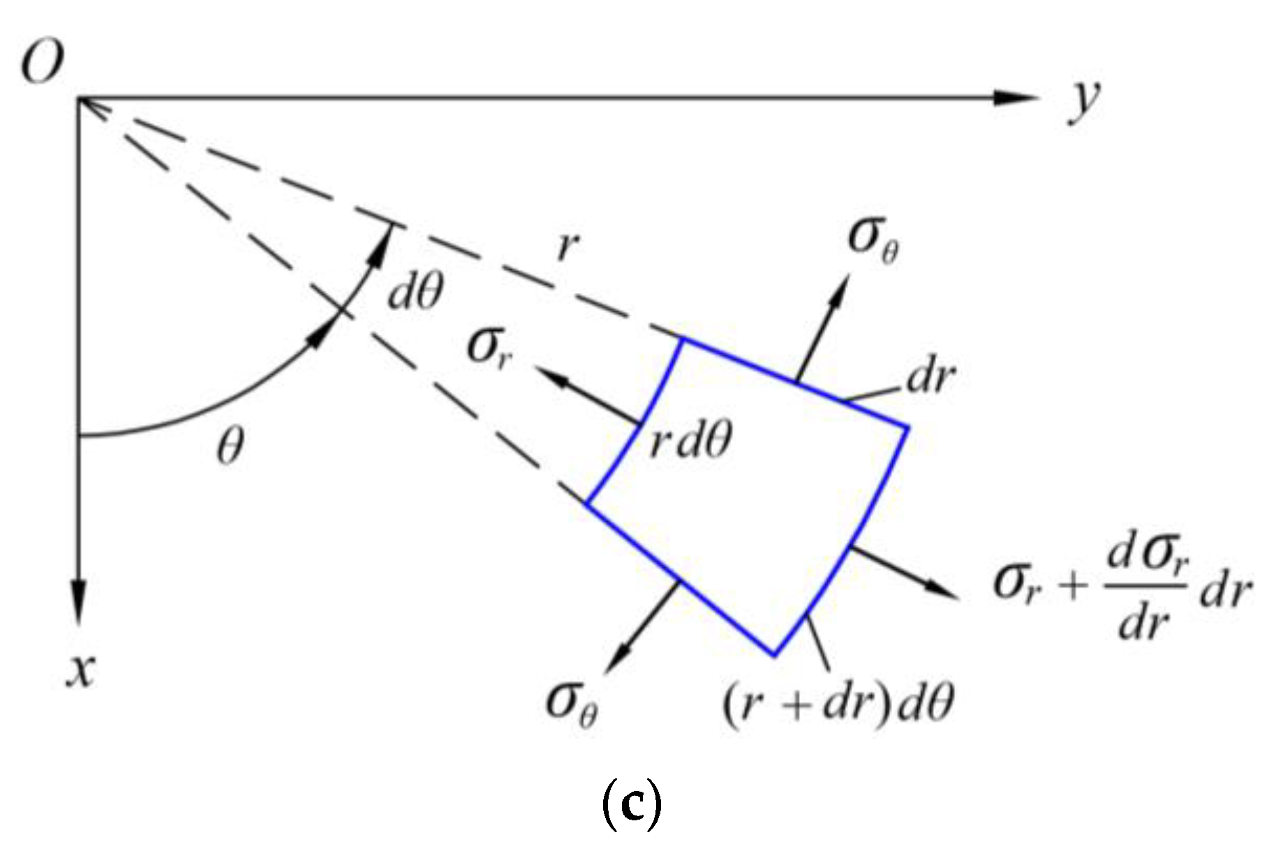
2.2. Description of Problem

As shown in Figure 2, a bimodular FGM thin circular plate is subjected to a transversely uniformly distributed load q, in which t is the plate thickness and a denotes the radius of the plate. The origin O of cylindrical coordinates system (O-rθz) is set at the plate center on the neutral layer; r, θ, and z denote the radial, circumferential, and transverse coordinates, respectively. For the reason of axisymmetry, θ is not depicted in Figure 2.
Note that in Figure 2, the dot-dashed line stands for the location of the unknown neutral layer of the plate, which is determined next. In general, due to the introduction of bimodular functionally graded materials, the neutral layer does not coincide with the geometrical middle plane of the plate. In Figure 2, t1 and t2 are the tensile thickness and compressive thickness, respectively, and the corresponding modulus of the material on the two thicknesses is the tensile modulus E+(z) and compressive modulus E(z), which is a function of z since the functionally graded property is varied along the thickness direction. To facilitate the application of the displacement variational method, the prescribed displacement should satisfy all displacement boundary conditions. Thus, the constraints for the thin circular plate are considered as fully fixed on its peripheral.
For the convenience of differential and integral operations, E+(z) and E(z) are defined as exponent-type functions [25], such that
E + ( z ) = E 0 e α 1 z / t ,   E ( z ) = E 0 e α 2 z / t ,
where α1 and α2 are two graded indices of the tensile zone and compressive one, respectively, and E0 is the elastic modulus on the neutral layer. From Equation (11), it is found that when α1 = α2 = 0 or z = 0, E+(z) = E(z) = E0. Meanwhile, according to common practice, the Poisson’s ratio is assumed as two constants, μ+ and μ, ignoring the gradient change along the direction of z.
In addition, the determination of the unknown neutral layer (t1 and t2) may be via two different conditions, according to our previous study [25]. One is the equilibrium condition, that is, the radial and circumferential normal forces acting on the differential element are zero; the other is the continuity condition, that is, the stresses acting on the neutral layer are continuous. In [25], the equilibrium condition gives
A 1 + 1 μ + + A 1 1 μ = 0 ,
while also in [25], the continuity condition gives
A 1 + 1 ( μ + ) 2 + A 1 1 ( μ ) 2 = 0 ,
in which
{ A 1 + = 0 t 1 z e α 1 z / t d z = [ ( t t 1 α 1 t 2 α 1 2 ) e α 1 t 1 / t + t 2 α 1 2 ] A 1 = t 2 0 z e α 2 z / t d z = [ ( t t 2 α 2 + t 2 α 2 2 ) e α 2 t 2 / t t 2 α 2 2 ] .
The obtainment process in detail for Equation (12a,b) may refer to our previous study [25], so there is no need to repeat the derivation process again. During the obtainment of Equation (12a,b), we first need to give the functional forms of E+(z) and E(z) for the subsequent integral operation, which is also the reason why Equation (11) is given first.
In addition, we note that for the two solutions concerning the neutral layer, it is obvious that the difference between them is slight due to the fact that the values for the Poisson’s ratio generally fall into the range of 0 to 0.3; also in Equation (12a,b), there is always a larger number compared to it (here, it is unit 1) before the Poisson’s ratio, thus making the influence of Poisson’s ratio on the solution small. Moreover, according to our previous study [35], if the influence of Poisson’s ratio is completely neglected, both Equation (12a,b) are reduced to A 1 + + A 1 = 0, which is exactly the solution used for the determination of the unknown neutral axis of bimodular FGM beams.

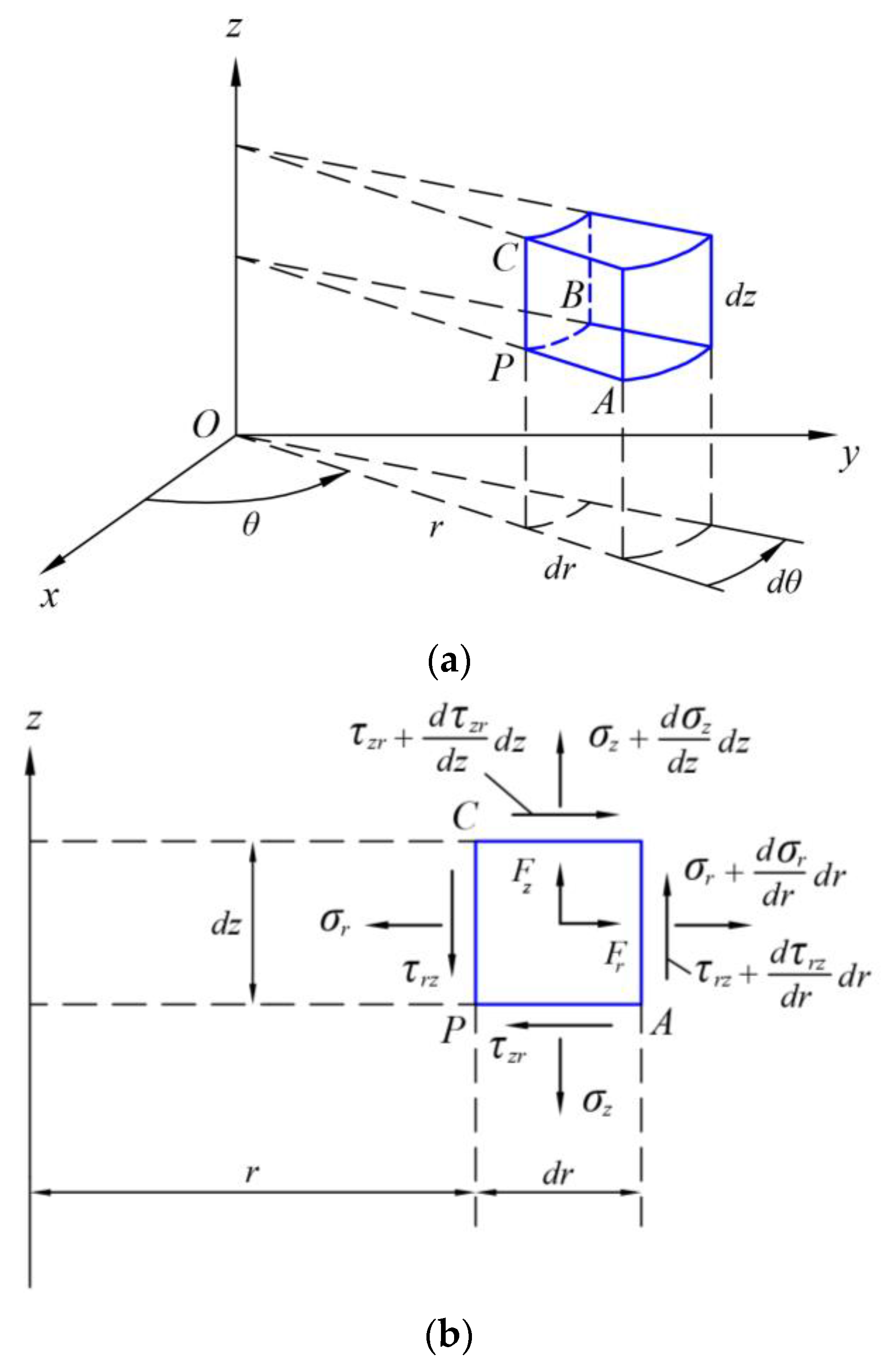
3. Geometrical and Physical Equations of Thin Circular Plates

Note that in a spatial axisymmetric problem, there exist four stress components in total, σr, σθ, σz, and τrz, and their corresponding strain components, εr, εθ, εz, and γrz; thus, the geometrical and physical relations will involve these stresses and strains. In the bending problem of thin plates, according to the classical Kirchhoff hypothesis, εz is negligibly small and γrz may be regarded as zero; thus, the geometrical and physical equations will finally involve the two main stresses, σr and σθ, as well as the corresponding strains, εr and εθ. Note that σz and τrz are not zero; they will participate in the equilibrium conditions; however, only the geometric and physical relations are discussed here.

3.1. Geometrical Equations under Large Deformation

The geometrical relation under small-deflection bending may be expressed in terms of the curvature [33] as follows, according to the classical Kirchhoff hypothesis:
ε r b = z ρ r ,   ε θ b = z ρ θ ,
where εrb and εθb are the radial and circumferential strain under small-deflection bending, respectively; ρr and ρθ are the curvature radius along the radial and circumferential directions, respectively; and in the case of small rotation angle, they are the following familiar forms [33]:
1 ρ r = d 2 w d r 2 ,   1 ρ θ = 1 r d w d r ,
where w is the transverse displacement or the deflection. Thus, the geometrical relation under small-deflection bending may be expressed in terms of w as follows:
ε r b = z d 2 w d r 2 ,   ε θ b = z 1 r d w d r .
At the same time, the geometrical relation between in-plane displacements and in-plane strain will give [33]
ε r m = d u r d r + 1 2 ( d w d r ) 2 ,   ε θ m = u r r ,
where εrm and εθm are the in-plane strains along the radial and circumferential directions, respectively; ur and w are the radial displacement and deflection, as indicated above. Finally, the total geometrical relation will give
{ ε r = ε r m + ε r b = d u r d r + 1 2 ( d w d r ) 2 z d 2 w d r 2 ε θ = ε θ m + ε θ b = u r r z 1 r d w d r .
If the plate is under small deflection, the above relation will change into the form of Equation (16). In the case of small deflection, only the bending effect is considered while the membrane effect is neglected.

3.2. Physical Equations

We suppose the radial and circumferential bending stresses in tensile and compressive zones are σ r b + / and σ θ b + / , respectively, in which the subscript b stands for the bending, and the stress–strain relations, in the tensile zone, will give
{ σ r b + = E + ( z ) 1 ( μ + ) 2 ( ε r b + μ + ε θ b ) σ θ b + = E + ( z ) 1 ( μ + ) 2 ( ε θ b + μ + ε r b )   ,   a t   0 z t 1 ,
and in the compressive zone,
{ σ r b = E ( z ) 1 ( μ ) 2 ( ε r b + μ ε θ b ) σ θ b = E ( z ) 1 ( μ ) 2 ( ε θ b + μ ε r b )   ,   a t   t 2 z 0 .
At the same time, we note that under large deformation, the in-plane stresses acting on the whole thickness of the cross-section are always tensile; thus. the membrane stress may be changed to σ r m + and σ θ m + , in which the subscript m stands for the membrane stress, and the elastic modulus and Poisson’s ratio may also be changed to E+(z) and μ+, respectively. The physical equation of in-plane deformation may be expressed, along the whole thickness direction, as
{ σ r m + = E + ( z ) 1 ( μ + ) 2 ( ε r m + μ + ε θ m ) σ θ m + = E + ( z ) 1 ( μ + ) 2 ( ε θ m + μ + ε r m )   ,   a t   t 2 z t 1 .
Next, the geometrical and physical equations obtained above are used for the establishment of the functional of energy.

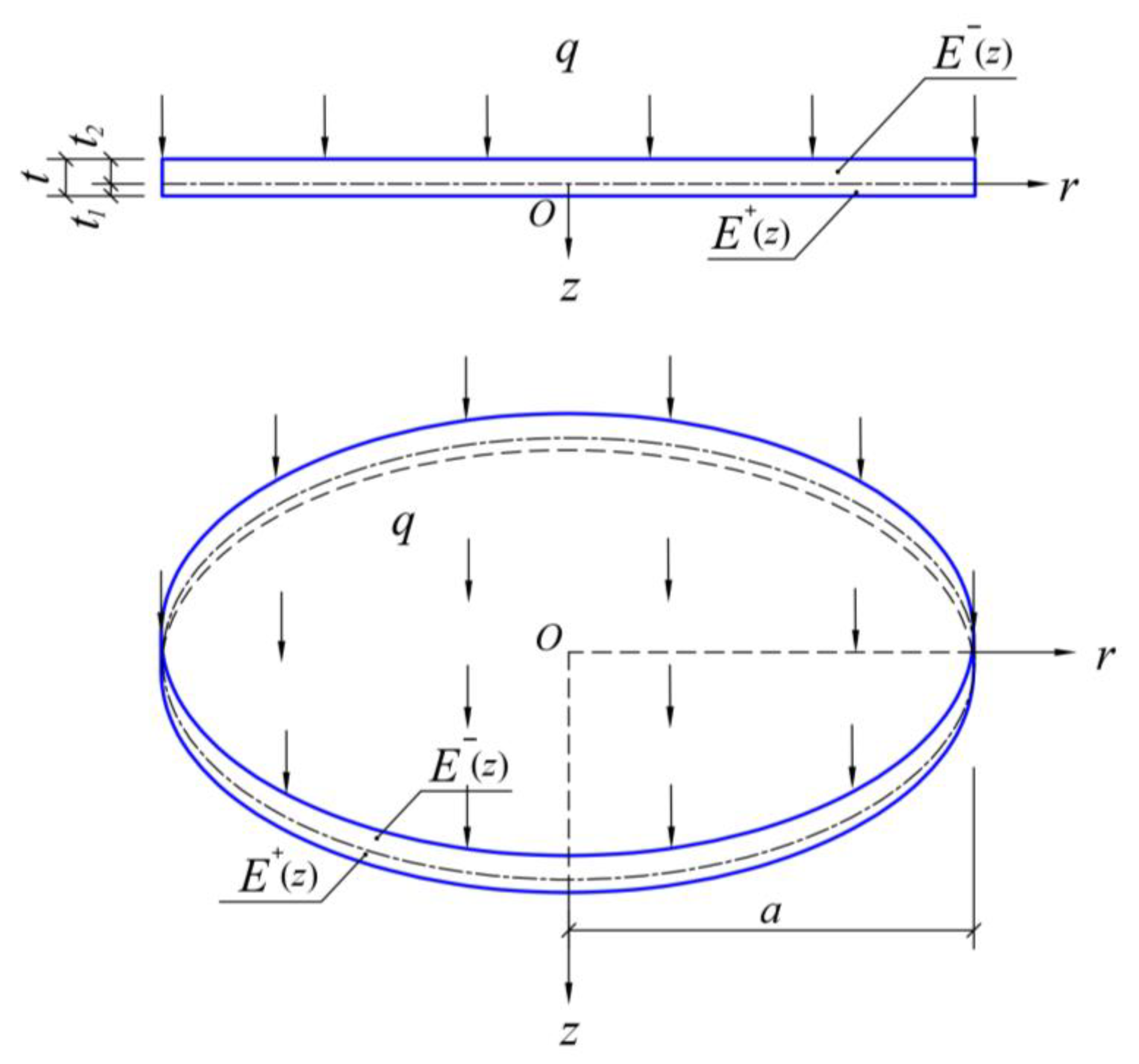
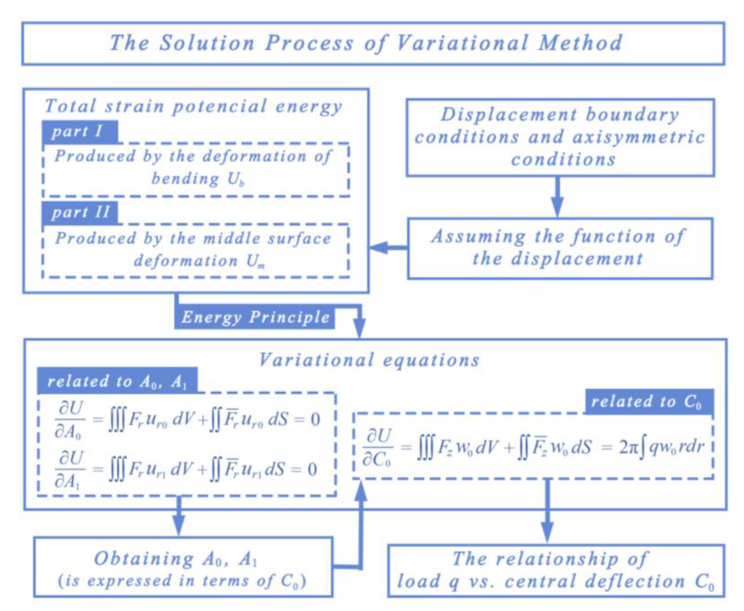
4. Displacement Variational Method

4.1. Total Strain Energy

The total strain energy, U, consists of the energy produced by the bending deformation, Ub, and the energy produced by the deformation of middle surface, Um, that is [30],
U = U b + U m ,
where the subscript b denotes the bending deformation and the subscript m denote the in-plane membrane deformation, which is consistent with the above notational conventions in geometrical and physical equations.
First, the strain energy produced by the middle surface deformation, Um, is computed as follows [30]:
U m = 1 2 V ( σ r m + ε r m + σ θ m + ε θ m ) d V .
Substituting Equation (20) into Equation (22) and also noticing that the lower limit and upper limit of the integral along the z direction are −t2 and t1, respectively, and dV = dzdS, Equation (22) may be written as
U m = 1 2 1 1 ( μ + ) 2 t 2 t 1 E + ( z ) d z S [ ( ε r m ) 2 + ( ε θ m ) 2 + 2 μ + ε r m ε θ m ] d S .
Also, substituting Equation (17) into Equation (23) will yield
U m = 1 2 1 1 ( μ + ) 2 t 2 t 1 E + ( z ) d z S { [ d u r d r + 1 2 ( d w d r ) 2 ] 2 + ( u r r ) 2 + 2 μ + u r r [ d u r d r + 1 2 ( d w d r ) 2 ] } d S .
Thus, Um is expressed in terms of ur and w. Considering Equation (11), we have
A 0 = t 2 t 1 E + ( z ) d z = t 2 t 1 E 0 e α 1 z / t d z = E 0 t α 1 ( e α 1 1 e α 1 t 2 / t ) ,
and also noting dS = rdθdr, Um may be further computed as
U m = π A 0 1 ( μ + ) 2 { r [ d u r d r + 1 2 ( d w d r ) 2 ] 2 + u r 2 r + 2 μ + u r [ d u r d r + 1 2 ( d w d r ) 2 ] } d r .
The energy produced by the bending deformation, Ub, can be derived by the above subareas in tension and compression, that is,
U b = 1 2 V + ( σ r b + ε r b + σ θ b + ε θ b ) d V + 1 2 V ( ( σ r b ε r b + σ θ b ε θ b ) ) d V .
Substituting Equation (19a,b) into Equation (27), we have
U b = 1 2 1 1 ( μ + ) 2 V + E + ( z ) [ ( ε r b ) 2 + ( ε θ b ) 2 + 2 μ + ε r b ε θ b ] d V + 1 2 1 1 ( μ ) 2 V E ( z ) [ ( ε r b ) 2 + ( ε θ b ) 2 + 2 μ ε r b ε θ b ] d V .
Substituting Equation (16) into Equation (28), and also noticing that the range of integrals in the tensile term is from 0 to t1 while the range in the compressive term is from −t2 to 0, we have
U b = 1 2 1 1 ( μ + ) 2 0 t 1 z 2 E + ( z ) d z [ ( d 2 w d r 2 ) 2 + ( 1 r d w d r ) 2 + 2 μ + 1 r d w d r d 2 w d r 2 ] d S + 1 2 1 1 ( μ ) 2 t 2 0 z 2 E ( z ) d z [ ( d 2 w d r 2 ) 2 + ( 1 r d w d r ) 2 + 2 μ 1 r d w d r d 2 w d r 2 ] d S .
If we let
{ A 2 + = 1 1 ( μ + ) 2 0 t 1 z 2 E + ( z ) d z = E 0 1 ( μ + ) 2 0 t 1 z 2 e α 1 z / t d z = E 0 1 ( μ + ) 2 [ ( 2 t 3 α 1 3 + t 1 2 t α 1 2 t 2 t 1 α 1 2 ) e α 1 t 1 / t 2 t 3 α 1 3 ] A 2 = 1 1 ( μ ) 2 t 2 0 z 2 E ( z ) d z = E 0 1 ( μ ) 2 t 2 0 z 2 e α 2 z / t d z = E 0 1 ( μ ) 2 [ ( 2 t 3 α 2 3 + t 2 2 t α 2 + 2 t 2 t 2 α 2 2 ) e α 2 t 2 / t + 2 t 3 α 2 3 ] ,
and also noting dS = rdθdr, Um may be finally computed as
U b = π A 2 + [ r ( d 2 w d r 2 ) 2 + 1 r ( d w d r ) 2 + 2 μ + d w d r d 2 w d r 2 ] d r + π A 2 [ r ( d 2 w d r 2 ) 2 + 1 r ( d w d r ) 2 + 2 μ d w d r d 2 w d r 2 ] d r .
Further, Equation (31) may be simplified if the peripheral of the circular plate is fully fixed. Note that the last term of the integrand in Equation (31) may be written as
0 a d 2 w d r 2 d w d r d r = 0 a d w d r d ( d w d r ) = 1 2 ( d w d r ) 2 | 0 a ,
in which a is the radius of the circular plate, as shown in Figure 2. If the peripheral of the circular plate is fully fixed, we may have dw/dr = 0 at r = a; at the same time, the axisymmetric condition also gives dw/dr = 0 at r = 0; it is obvious that, lastly, we have
0 a d 2 w d r 2 d w d r d r = 0 .
Thus, Equation (32) is simplified as
U b = π ( A 2 + + A 2 ) [ r ( d 2 w d r 2 ) 2 + 1 r ( d w d r ) 2 ] d r = π D [ r ( d 2 w d r 2 ) 2 + 1 r ( d w d r ) 2 ] d r ,
in which D* is exactly the bending stiffness of the bimodular FGM plate,
D = A 2 + + A 2 ,
which indicates that the bending stiffness is still obtained via the derivation of bending strain energy, not via the equilibrium relation in our previous study [25].
Finally, we obtain the total strain potential energy, U,
U = U b + U m = π D [ r ( d 2 w d r 2 ) 2 + 1 r ( d w d r ) 2 ] d r + π A 0 1 ( μ + ) 2 { r [ d u r d r + 1 2 ( d w d r ) 2 ] 2 + u r 2 r + 2 μ + u r [ d u r d r + 1 2 ( d w d r ) 2 ] } d r ,
which is expressed in terms of the displacement components, ur and w. Note that for the case of small deflection, in Equation (36), only the bending term Ub is retained, while the membrane force term Um is omitted.

4.2. Ritz Method

For the large-deformation problem of thin circular plates, we take the following displacement components (note that due to the axisymmetry, uθ = 0):
u r = m A m u r m ,   w = m C m w m ,
where Am and Cm are the independent coefficients, and urm and wm are the specified functions that are equal to zero on the boundaries. Thus, the displacements, ur and w, always satisfy displacement boundary conditions. According to the variational method in Section 2.1 and also considering Equation (10), the following two variational equations may be obtained:
U A m = F r u r m d V + F r ¯ u r m d S = 0
and
U C m = F z w m d V + F z ¯ w m d S = q w m d S = 2 π q w m r d r ,
where F z ¯ = q . Equations (38) and (39) are used for solving Am and Cm. We adopt the following forms of the radial displacement and deflection:
u r = ( 1 r a ) r a [ A 0 + A 1 r a + A 2 ( r a ) 2 + ]
and
w = ( 1 r 2 a 2 ) 2 [ C 0 + C 1 ( 1 r 2 a 2 ) + C 2 ( 1 r 2 a 2 ) 2 + ] .
Obviously, regardless of how the coefficients are chosen, the displacements satisfy the boundary conditions of displacement at the peripheral:
u r = 0 ,   w = 0 ,   d w d r = 0     a t   r = a ,
and the axisymmetric conditions at the center:
u r = 0 ,     d w d r = 0     a t   r = 0 .
According to the conclusion from [30,33,34], by taking the first few terms, the variational method can give satisfactory results. Thus, in the next computation, for convenience, we take A0 and A1 in Equation (40) and C0 in Equation (41) and then substitute these two displacement formulas into Equation (34):
U b = 32 π D 3 a 2 C 0 2 .
And substituting these displacement formulas into Equation (26), we have
U m = E 0 π t 1260 [ 1 ( μ + ) 2 ] α 1 a 2 e α 1 t 2 / t ( e α 1 1 ) × ( 328 μ + a A 0 C 0 2 + 176 μ + a A 1 C 0 2 + 315 a 2 A 0 2 + 378 a 2 A 0 A 1 184 a A 0 C 0 2 + 147 a 2 A 1 2 + 16 a A 1 C 0 2 + 384 C 0 4 ) .
In addition,
2 π q w m r d r = 2 π q 0 a ( 1 r 2 a 2 ) 2 r d r = π 3 q a 2 .
According to Equations (21), (38), and (39), we have
A 0 ( U b + U m ) = 0 ,   A 1 ( U b + U m ) = 0 ,
and
C 0 ( U b + U m ) = π 3 q a 2 .
Substituting Equations (44) and (45) into Equation (47), we have
{ U A 0 = E 0 π t 1260 [ 1 ( μ + ) 2 ] α 1 a 2 e α 1 t 2 / t ( e α 1 1 ) ( 328 μ + a C 0 2 + 630 a 2 A 0 + 378 a 2 A 1 184 a C 0 2 ) = 0 U A 1 = E 0 π t 1260 [ 1 ( μ + ) 2 ] α 1 a 2 e α 1 t 2 / t ( e α 1 1 ) ( 176 μ + a C 0 2 + 378 a 2 A 0 + 294 a 2 A 1 + 16 a C 0 2 ) = 0 ,
and then we express A0 and A1 with C0:
A 0 = C 0 2 126 a ( 89 μ + 179 ) ,     A 1 = C 0 2 42 a ( 13 μ + 79 ) .
At the same time, substituting Equations (44)–(46) into Equation (48), we have
E 0 π t 1260 [ 1 ( μ + ) 2 ] α 1 a 2 e α 1 t 2 / t ( e α 1 1 ) ( 656 μ + a A 0 C 0 + 352 μ + a A 1 C 0 368 a A 0 C 0 + 32 a A 1 C 0 + 1536 C 0 3 ) + 64 π D 3 a 2 C 0 π 3 q a 2 = 0 .
Substituting Equation (50) into Equation (51), we finally have
H C 0 3 + 64 D 3 C 0 = 1 3 q a 4 ,
where
H = 2 E 0 t ( e α 1 1 ) 19845 [ 1 ( μ + ) 2 ] α 1 e α 1 t 2 / t [ 2791 ( μ + ) 2 4250 μ + 7505 ] .
Thus, C0 may be solved and, according to Equation (50), A0 and A1 may also be obtained accordingly. Once the displacements become known, the corresponding stresses and strains may be obtained. Note that C0 also stands for the central deflection of the thin circular plate; therefore, Equation (52) presents the important relationship of load vs. central deflection. In order to better clarify the solution process of the variational method, we add a flow block diagram for reference (please see Figure 3).
In addition, we note that the above solution is derived on the simple form of the displacement functions ur and w; that is, A0 and A1 are taken in Equation (40), and only C0 is taken in Equation (41). Although the next comparison with the numerical simulation will show its reliability in the case of small-number terms, for higher precision, more terms in displacement functions ur and w are necessary; thus, the computation for more terms was also conducted. But, for the sake of coherence of this study, we put this part into Appendix A for interested readers, in which A0, A1, and A2 are taken in Equation (40) and C0 and C1 are taken in Equation (41).

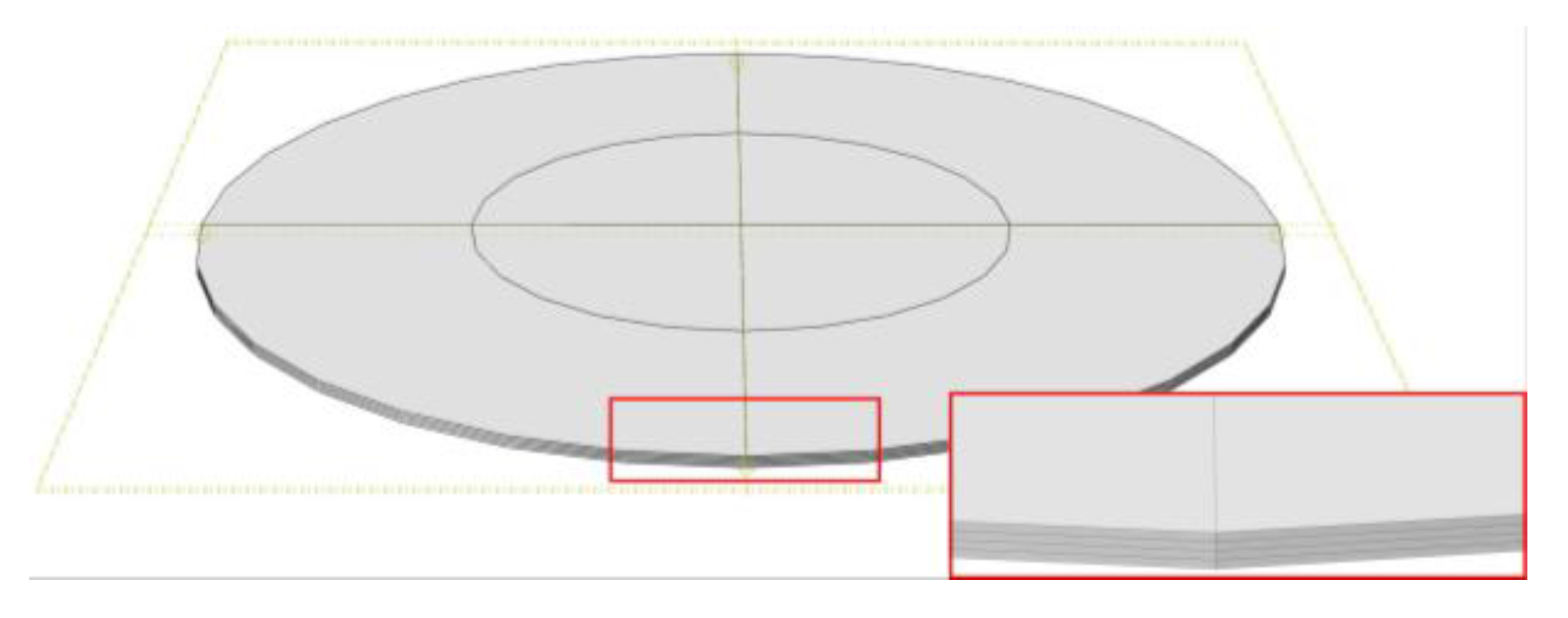
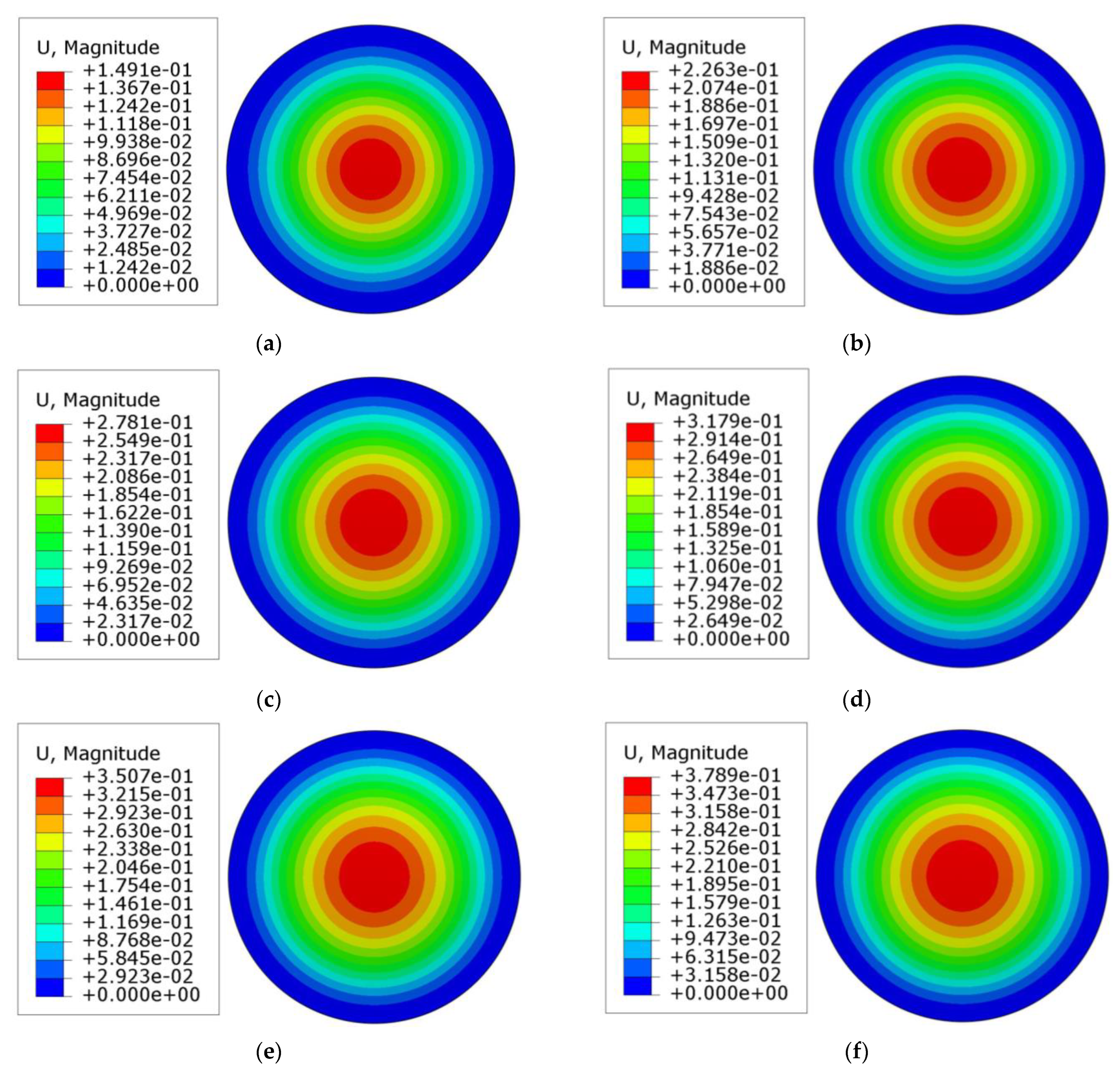
5. Numerical Simulation and Comparison with Variational Solution

We use the software ABAQUS6.14.4 to conduct the numerical simulation. When constructing the computational model of a thin circular plate, the first step is to create the three-dimensional solid diagram based on the real shape and size. In our study, the radius of the thin plate, a, is taken as 10 m, and the thickness of the plate, t, is taken as 0.2 m. The peripheral of the circular plate is fully fixed and the load magnitudes take different values, ranging from 10 kPa to 200 kPa, with an interval of 10 kPa. The given values in the numerical simulation are listed in Table 1. A three-dimensional solid element with eight nodes, C3D8, is adopted to conduct the numerical computation. Figure 4 shows the grid division, the loading, and the boundary conditions.
In our numerical computation, the simulation for bimodular functionally graded materials presents a slight degree of complexity. In ABAQUS6.14.4 software, the realization for functionally graded properties of materials is by layering, but before layering, in consideration of the bimodular effect, we must determine the position of the neutral layer first, that is, only after the subareas are in tension and compression can we effectively layer. To this end, we need to use Equation (12a) or (12b) and the data from Table 1 to determine the tensile thickness and compressive one first, which give t1 = 0.4917t and t2 = 0.5083t, respectively, where t is the thickness of the plate. Then, the thin circular plate is divided into eight layers along the thickness direction (see Figure 5), taking the middle modulus as the average modulus of this layer. The moduli of elasticity and Poisson’s ratios for these eight layers are computed and listed in Table 2, which are used for the property module during the material editing.
Figure 6 shows some representative displacement nephograms under different magnitudes of load, including 20 kPa, 40 kPa, 60 kPa, 80 kPa, 100 kPa, and 120 kPa. From Figure 6, it is easy to see that the maximum deflection occurs at the center of the thin circular plate, as we predicted; the central deflection gradually increases with the increase in load magnitude; and from the center of the plate to the edge of the plate, the deflection gradually decreases, as predicted in our theoretical solution.
Table 3 lists the central deflection values under different load magnitudes (from q = 10 kPa to q = 200 kPa, with an interval of 10 kPa). For an effective comparison, in Table 3, we also list two other groups of value from different theoretical solutions, the variational solution in this study and the perturbation solution in our previous study [26], in which the results from the variational solution are obtained via Equation (52) in this study; the results from the perturbation solution are based on Equation (104) in [26]. By comparing the values of central deflection in Table 3, it is easily found that the values from the three solutions are basically consistent, but there still exist small differences between them. However, the differences are negligibly small and generally acceptable, which verifies the validity of the variational method.

6. Results and Discussion

6.1. Numerical Comparision of Three Solutions

From the current results, it is found that if the numerical solution can be regarded as a standard to test the validity of two theoretical solutions, the perturbation solution is closest, followed by the variational solution. The values from the variational solution are slightly larger than the values from the perturbation solution, which agrees with the results of classical large-deflection solutions from [29,30]. As indicated in the Introduction, in the literature, both Chien’s perturbation solution [29] and the variational solution [30] give satisfactory results. In Chien’s perturbation solution [29], the relationship between load and maximum deflection gives
q a 4 64 D = w 0 [ 1 + 0.544 ( w 0 t ) 2 ] ,
while, in the variational solution [30], the same relationship is
q a 4 64 D = w 0 [ 1 + 0.486 ( w 0 t ) 2 ] ,
where a is the radius of a thin circular plate, t is the plate thickness, w0 is the central deflection, q is the uniformly distributed loads, and D is the bending stiffness of the plate. It is readily found that they are quite close. In addition, we note that if other quantities in this relationship take the same values, the value of the maximum deflection from the variational solution is a little greater than the value from the perturbation solution.
The above conclusion is drawn on the basis of the variation solution with fewer terms. If the variation solution with more terms is taken, another phenomenon should be noticed. From the data of the second column marked with footer 2, it is easy to see that if more terms in the displacement functions are taken, the precision of the variational solution will be significantly improved, even exceeding that of the perturbation solution.
It should be noted here that the observed discrepancies resulting from the variational method and FEM method may come down to the fact that, apart from differences in the calculation methods themselves, it comes from different simulated models of the material properties. In the Ritz method, the bimodular functionally graded properties are considered as, for the bimodular effect, the subarea in tension and compression is used, while for the functionally graded property, in each tensile or compressive area, two smooth and continuous functions ((Equation (11)) are adopted. At the same time, in the FEM method, the subarea in tension and compression is still used for the bimodular effect, but the functionally graded property is realized by the layering along the direction of plate thickness; thus, the difference is inevitable. We can speculate that if more layers are adopted, the simulation of materials is likely to be closer to the continuous function change, like Equation (11). However, considering the computational efforts and time, only eight layers were adopted in our present study. In future work, more layers can be adopted to obtain a more precise result.

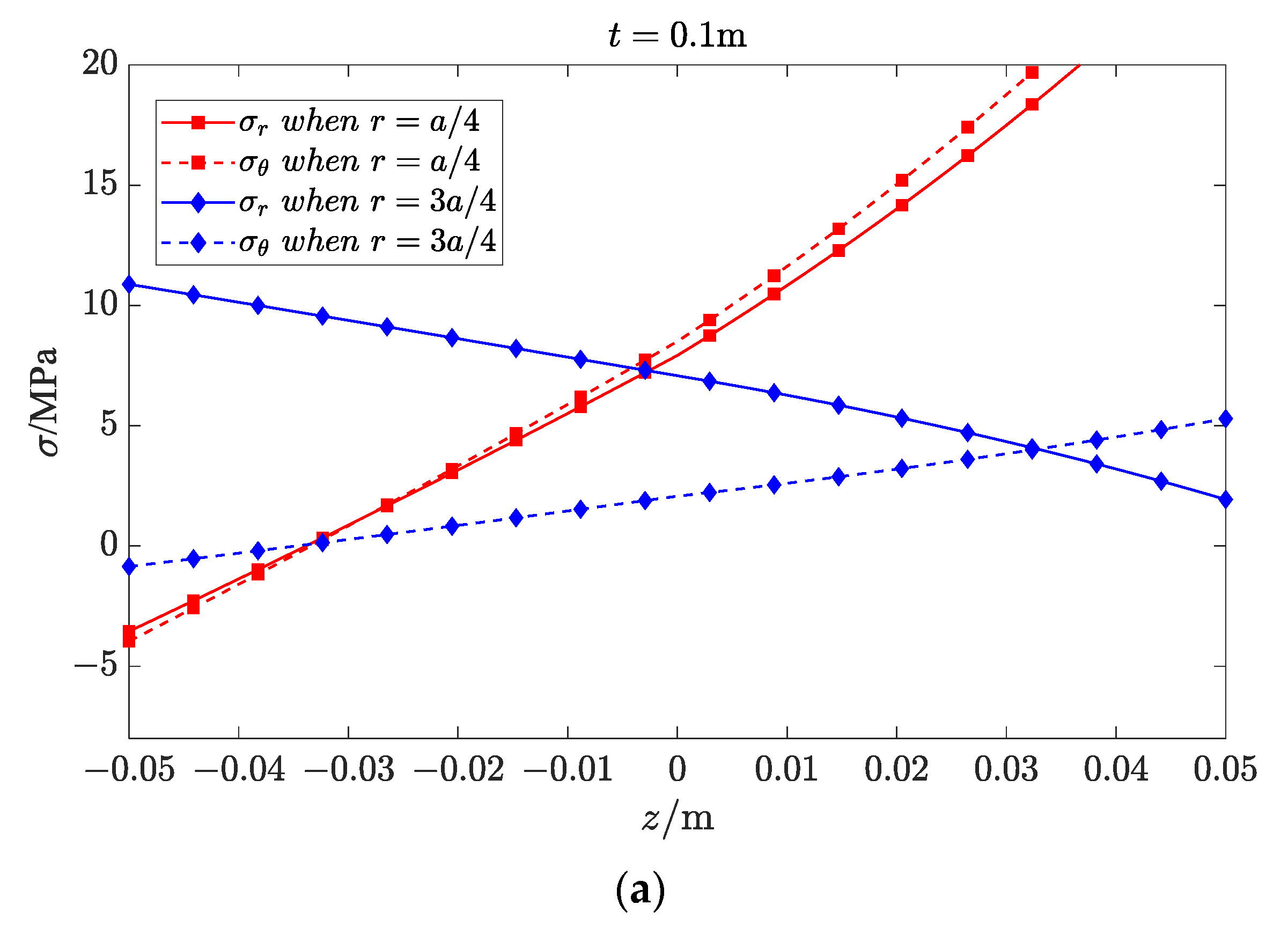
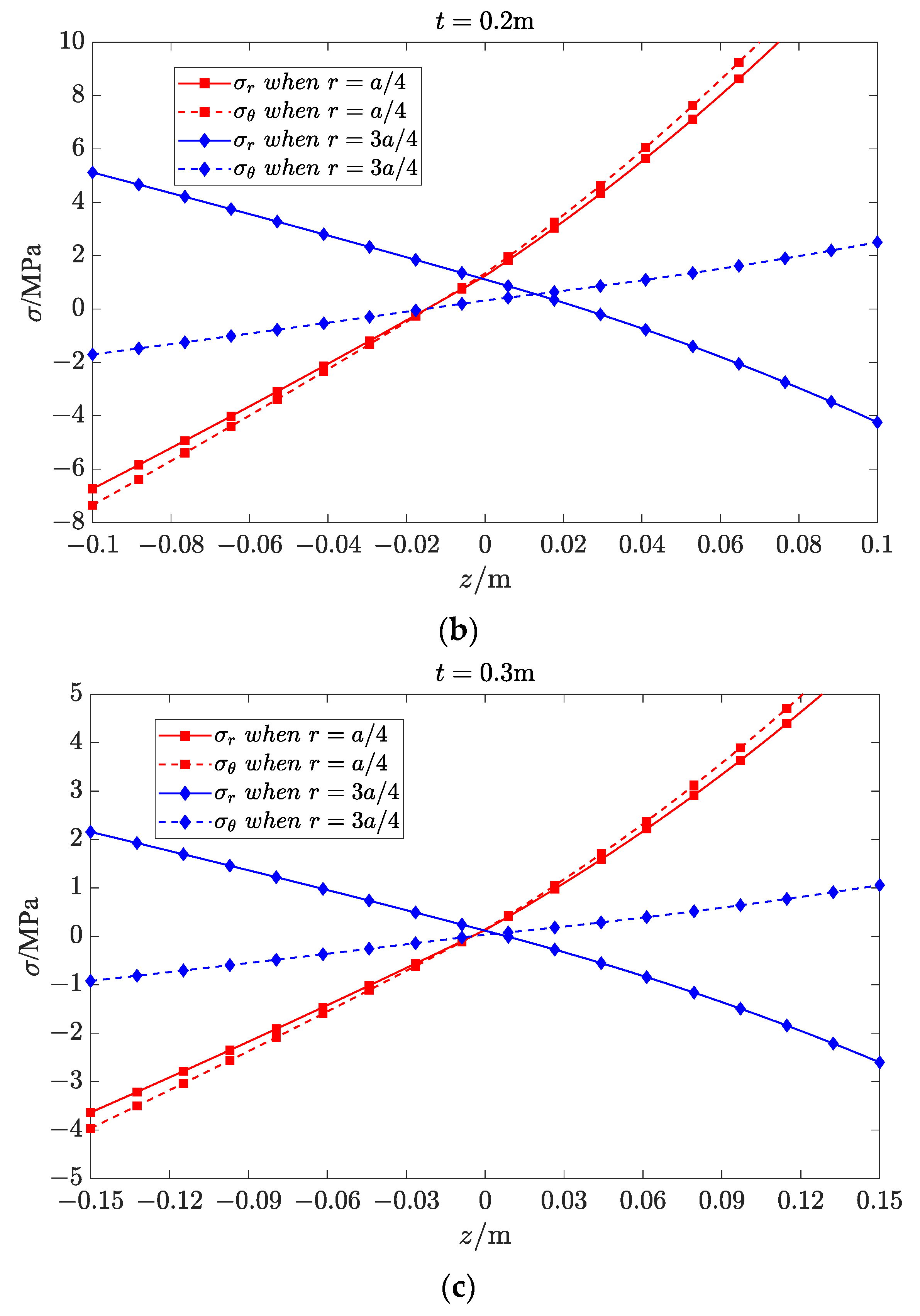
6.2. Stress Variation along Plate Thickness

In order to investigate the influence of plate thickness on the radial and circumferential stresses, we take three different thickness values, 0.1 m, 0.2 m, and 0.3 m, to carry out the numerical computation, and other taken values may refer to Table 1, in which the load intensity is taken as 10 kPa. At the same time, we take two different survey locations, that is, r = a/4 and r = 3a/4, where a is the radius of the circular plate, to investigate the influence of different radial locations on stresses. The numerical results are plotted in Figure 7, in which Figure 7a–c correspond to the thickness cases of t = 0.1 m, t = 0.2 m, and t = 0.3 m.
From Figure 7, the following two trends may be found. (i) The stress distribution trend of radial and circumferential stresses under different plate thicknesses is basically the same, that is, when r = a/4 (near the plate center), the differences between the radial and circumferential stresses tend to be smaller; when r = 3a/4 (near the plate edge), the differences between the radial and circumferential stresses tend to be larger, which may be due to the influence of boundary constraints. (ii) When the plate becomes thinner (t = 0.1 m), the radial and circumferential stresses both tend to be tensile, indicating that the membrane stress is dominant in thinner plates; when the plate becomes thicker (t = 0.3 m), the tensile area and compressive area appear distinct, showing that the bending stress is dominant in thicker plates. This phenomenon is also consistent with our expectations.

7. Conclusions

In this paper, the displacement variational method is used to solve the large-deformation problem of bimodular functionally graded thin plates. In order to facilitate the application of the variational method, the physical equations of the bimodular functionally graded material and the geometric equation under large deformation are first given. The total strain potential energy is expressed as the displacement component, which opens up the possibility for the realization of the Ritz method. Finally, the analytical result is verified by numerical simulation. The following three conclusions can be drawn.
(i)
The numerical simulation results verify the validity of the perturbation solution obtained in our previous study and the variational solution presented in this study.
(ii)
The perturbation method and variational method are both, in terms of nature, theoretical, being able to give useful analytical expressions that are convenient for use in the analysis and design. However, the variational method based on the energy principle avoids the establishment of an equation of equilibrium, which is necessary in the perturbation method yet.
(iii)
Compared with the traditional variational method, the improvement on this method in this study lies mainly in such a fact that the derivation of total strain energy is somewhat complicated due to the introduction of bimodular functionally graded materials and structural large deformation. In addition, the bending stiffness of the bimodular FGM plate may also be obtained from the derivation of total strain energy, but not necessarily from the conditions of equilibrium.
The results presented in this study are helpful for the refined analysis and optimized design of flexible thin plate structures, which are composed of functionally graded materials, while at the same time, the bimodular effect of materials is relatively obvious and cannot be ignored.
In the end, it should be pointed out again that Ambartsumyan’s bimodular model is established on the criterion of positive–negative signs of principal stresses. This fact makes it very difficult to use this model in structural analysis, because, except for a very few cases, the state of principal stress at any point in the structure is different each other under the action of external load. Fortunately, the proposal of a simplified mechanical model on a subarea in tension and compression makes it possible to use Ambartsumyan’s bimodular model in structural analysis. While, at the same time, the material model also deviates from the original definition, this may be seen as an imperfection of the method. In the future, we will try to establish a simplified mechanical model that satisfies the requirements of structural analysis and is closer to the original material model. This work is in progress.

Author Contributions

Conceptualization, X.-T.H. and J.-Y.S.; methodology, X.-T.H., X.-G.W. and J.-C.A.; software, X.-G.W., B.P. and J.-C.A.; formal analysis, X.-T.H., X.-G.W. and J.-C.A.; writing—original draft preparation, X.-T.H. and X.-G.W.; writing—review and editing, B.P., J.-C.A. and J.-Y.S.; visualization, X.-G.W., B.P. and J.-C.A.; funding acquisition, X.-T.H. and J.-Y.S. All authors have read and agreed to the published version of the manuscript.

Funding

The research described in this paper was financially supported by the National Natural Science Foundation of China (Grant Nos. 11572061 and 11772072).

Data Availability Statement

Not applicable.

Conflicts of Interest

The authors declare no conflict of interest.

Appendix A

If more terms in displacement functions ur and w are taken, that is, A0, A1, and A2 are taken in Equation (40), and C0 and C1 are taken in Equation (41), we have the following displacement:
u r = ( 1 r a ) r a [ A 0 + A 1 r a + A 2 ( r a ) 2 ]
and
w = ( 1 r 2 a 2 ) 2 [ C 0 + C 1 ( 1 r 2 a 2 ) ] .
Substituting them into Equations (34) and (26), respectively, we have
U b = 32 π D 3 a 2 C 0 2 + 16 π D a 2 C 0 C 1 + 48 π D 5 a 2 C 1 2 .
and
U m = E 0 π t [ 1 ( μ + ) 2 ] α 1 e α 1 t 2 / t ( e α 1 1 ) × [ 13 168 A 2 2 + 7 60 A 1 2 + 3 10 A 0 A 1 + 1 5 A 0 A 2 + 19 105 A 1 A 2 + 32 105 a 2 C 0 4 + 18 55 a 2 C 1 4 + 6 5 a 2 C 0 C 1 3 + 1 4 A 0 2 + 1 3465 a ( 284 μ + A 2 C 0 2 + 212 A 2 C 0 2 ) + 1 315 a ( 44 μ + A 1 C 0 2 + 82 μ + A 0 C 0 2 46 A 0 C 0 2 + 4 A 1 C 0 2 ) + 1 385 a ( 102 μ + A 1 C 0 C 1 + 206 μ + A 0 C 0 C 1 ) + 1 5005 a ( 886 A 2 C 0 C 1 + 1467 μ + A 0 C 1 2 + 678 μ + A 1 C 1 2 + 346 μ + A 2 C 1 2 + 722 μ + A 2 C 0 C 1 69 A 0 C 1 2 + 526 A 2 C 1 2 + 498 A 1 C 1 2 ) + 1 77 a ( 10 A 1 C 0 C 1 10 A 0 C 0 C 1 ) + 1 7 a 2 ( 12 C 0 2 C 1 2 + 8 C 0 3 C 1 ) ] .
In addition,
{ 2 π q w m = 0 r d r = 2 π q 0 a ( 1 r 2 a 2 ) 2 r d r = π 3 q a 2 2 π q w m = 1 r d r = 2 π q 0 a ( 1 r 2 a 2 ) 3 r d r = π 4 q a 2
According to Equations (21), (38), and (39), we have
{ A 0 ( U b + U m ) = 0 A 1 ( U b + U m ) = 0 A 2 ( U b + U m ) = 0
and
{ C 0 ( U b + U m ) = π 3 q a 2 C 1 ( U b + U m ) = π 4 q a 2 .
Substituting Equations (A3) and (A4) into Equation (A6), we have
{ U A 0 = E 0 π t [ 1 ( μ + ) 2 ] α 1 e α 1 t 2 / t ( e α 1 1 ) ( 1 2 A 0 + 206 μ + 385 a C 0 C 1 + 3 10 A 1 + 1 5 A 2 + 82 μ + 315 a C 0 2 + 1467 μ + 5005 a C 1 2 10 77 a C 0 C 1 46 315 a C 0 2 69 5005 a C 1 2 ) = 0 U A 1 = E 0 π t [ 1 ( μ + ) 2 ] α 1 e α 1 t 2 / t ( e α 1 1 ) ( 7 30 A 1 + 102 μ + 385 a C 0 C 1 + 3 10 A 0 + 19 105 A 2 + 44 μ + 315 a C 0 2 + 678 μ + 5005 a C 1 2 + 10 77 a C 0 C 1 + 4 315 a C 0 2 + 498 5005 a C 1 2 ) = 0 U A 2 = E 0 π t [ 1 ( μ + ) 2 ] α 1 e α 1 t 2 / t ( e α 1 1 ) ( 13 84 A 2 + 722 μ + 5005 a C 0 C 1 + 1 5 A 0 + 19 105 A 1 + 284 μ + 3465 a C 0 2 + 886 5005 a C 0 C 1 + 346 μ + 5005 a C 1 2 + 212 3465 a C 0 2 + 526 5005 a C 1 2 ) = 0
And then we express A0, A1, and A2 with C0 and C1:
{ A 0 = 1 180,180 a ( 93,990 μ + C 0 2 + 249,516 μ + C 0 C 1 + 167,931 μ + C 1 2 206,050 C 0 2 553,824 C 0 C 1 350,145 C 1 2 ) A 1 = 1 25,740 a ( 11,050 μ + C 0 2 + 5508 μ + C 0 C 1 8307 μ + C 1 2 + 19,890 C 0 2 + 149,328 C 0 C 1 + 124,425 C 1 2 ) A 2 = 8 6435 a ( 520 μ + C 0 2 + 891 μ + C 0 C 1 + 306 μ + C 1 2 780 C 0 2 + 1341 C 0 C 1 + 1980 C 1 2 ) .
At the same time, substituting Equations (A3) and (A4) into Equation (A7), we have
D ( 16 π a 2 C 1 + 64 π 3 a 2 C 0 ) + E 0 π t [ 1 ( μ + ) 2 ] α 1 e α 1 t 2 / t ( e α 1 1 ) × ( 722 μ + 5005 a A 2 C 1 + 102 μ + 385 a A 1 C 1 + 206 μ + 385 a A 0 C 1 + 128 105 a 2 C 0 3 + 568 μ + 3465 a A 2 C 0 + 88 μ + 315 a A 1 C 0 + 164 μ + 315 a A 0 C 0 + 886 5005 a A 2 C 1 + 10 77 a A 1 C 1 10 77 a A 0 C 1 92 315 a A 0 C 0 + 8 315 a A 1 C 0 + 424 3465 a A 2 C 0 + 24 7 a 2 C 0 C 1 2 + 24 7 a 2 C 0 2 C 1 + 6 5 a 2 C 1 3 ) = π q a 2 3 ,
and
D ( 16 π a 2 C 0 + 96 π 5 a 2 C 1 ) + E 0 π t [ 1 ( μ + ) 2 ] α 1 e α 1 t 2 / t ( e α 1 1 ) × ( 722 μ + 5005 a A 2 C 0 + 102 μ + 385 a A 1 C 0 + 206 μ + 385 a A 0 C 0 + 72 55 a 2 C 1 3 + 1356 μ + 5005 a A 1 C 1 + 886 5005 a A 2 C 0 + 2934 μ + 5005 a A 0 C 1 + 10 77 a A 1 C 0 10 77 a A 0 C 0 + 692 μ + 5005 a A 2 C 1 138 5005 a A 0 C 1 + 24 7 a 2 C 0 2 C 1 + 8 7 a 2 C 0 3 + 1052 5005 a A 2 C 1 + 996 5005 a A 1 C 1 + 18 5 a 2 C 0 C 1 2 ) = π q a 2 4 ,
Substituting Equation (A9) into Equations (A10) and (A11), we finally obtain the expressions of C0 and C1. Since the expressions are too complex, they are not given here. At the same time, according to Equation (A2), if we let r = 0, the central deflection or the maximum deflection of the circular plate will be
w 0 = C 0 + C 1 .

References

  1. Jones, R.M. Stress-strain relations for materials with different moduli in tension and compression. AIAA J. 1977, 15, 16–23. [Google Scholar] [CrossRef]
  2. Koizumi, M. Functionally gradient materials the concept of FGM. Ceram. Trans. 1993, 34, 3–10. [Google Scholar]
  3. Gong, Y.; Mei, Y.; Liu, J. Capillary adhesion of a circular plate to solid: Large deformation and movable boundary condition. Int. J. Sci. Mech. 2017, 126, 222–228. [Google Scholar] [CrossRef]
  4. Huang, X.; Wang, M.; Feng, Y.; Wang, X.; Qiu, X. Finite deformation analysis of the elastic circular plates under pressure loading. Thin-Walled Struct. 2023, 188, 110864. [Google Scholar] [CrossRef]
  5. Barak, M.M.; Currey, J.D.; Weiner, S.; Shahar, R. Are tensile and compressive Young’s moduli of compact bone different. J. Mech. Behav. Biomed. Mater. 2009, 2, 51–60. [Google Scholar] [CrossRef] [PubMed]
  6. Destrade, M.; Gilchrist, M.D.; Motherway, J.A.; Murphy, J.G. Bimodular rubber buckles early in bending. Mech. Mater. 2010, 42, 469–476. [Google Scholar] [CrossRef] [Green Version]
  7. Jones, R.M. Apparent flexural modulus and strength of multimodulus materials. J. Compos. Mater. 1976, 10, 342–354. [Google Scholar] [CrossRef]
  8. Bert, C.W. Models for fibrous composites with different properties in tension and compression. ASME J. Eng. Mater. Technol. 1977, 99, 344–349. [Google Scholar] [CrossRef]
  9. Ambartsumyan, S.A. Elasticity Theory of Different Moduli; Wu, R.F.; Zhang, Y.Z., Translators; China Railway Publishing House: Beijing, China, 1986. [Google Scholar]
  10. Reddy, J.N.; Chao, W.C. Nonlinear bending of bimodular material plates. Int. J. Solids Struct. 1983, 19, 229–237. [Google Scholar] [CrossRef]
  11. Zinno, R.; Greco, F. Damage evolution in bimodular laminated composite under cyclic loading. Compos. Struct. 2001, 53, 381–402. [Google Scholar] [CrossRef]
  12. Khan, A.H.; Patel, B.P. Nonlinear periodic response of bimodular laminated composite annular sector plates. Compos. Part B-Eng. 2019, 169, 96–108. [Google Scholar] [CrossRef]
  13. Yao, W.J.; Ye, Z.M. Analytical solution for bending beam subject to lateral force with different modulus. Appl. Math. Mech. (Engl. Ed.) 2004, 25, 1107–1117. [Google Scholar]
  14. Zhao, H.L.; Ye, Z.M. Analytic elasticity solution of bi-modulus beams under combined loads. Appl. Math. Mech. (Engl. Ed.) 2015, 36, 427–438. [Google Scholar] [CrossRef]
  15. He, X.T.; Cao, L.; Wang, Y.Z.; Sun, J.Y.; Zheng, Z.L. A biparametric perturbation method for the Föppl-von Kármán equations of bimodular thin plates. J. Math. Anal. Appl. 2017, 455, 1688–1705. [Google Scholar] [CrossRef]
  16. Ye, Z.M.; Chen, T.; Yao, W.J. Progresses in elasticity theory with different moduli in tension and compression and related FEM. Mech. Eng. 2004, 26, 9–14. [Google Scholar]
  17. Du, Z.L.; Zhang, Y.P.; Zhang, W.S.; Guo, X. A new computational framework for materials with different mechanical responses in tension and compression and its applications. Int. J. Solids Struct. 2016, 100–101, 54–73. [Google Scholar] [CrossRef]
  18. Ma, J.W.; Fang, T.C.; Yao, W.J. Nonlinear large deflection buckling analysis of compression rod with different moduli. Mech. Adv. Mater. Struct. 2019, 26, 539–551. [Google Scholar] [CrossRef]
  19. Almajid, A.; Taya, M.; Hudnut, S. Analysis of out-of-plane displacement and stress field in a piezocomposite plate with functionally graded microstructure. Int. J. Solids Struct. 2001, 38, 3377–3391. [Google Scholar] [CrossRef]
  20. Kumar, S.; Murthy Reddy, K.V.V.S.; Kumar, A.; Rohini Devi, G. Development and characterization of polymer–ceramic continuous fiber reinforced functionally graded composites for aerospace application. Aerosp. Sci. Technol. 2013, 26, 185–191. [Google Scholar] [CrossRef]
  21. Maalej, M.; Ahmed, S.F.U.; Paramasivam, P. Corrosion durability and structural response of functionally-graded concrete beams. J. Adv. Concr. Technol. 2003, 1, 307–316. [Google Scholar] [CrossRef] [Green Version]
  22. Rabbani, V.; Hodaei, M.; Deng, X.; Lu, H.; Hui, D.; Wu, N. Sound transmission through a thick-walled FGM piezo-laminated cylindrical shell filled with and submerged in compressible fluids. Eng. Struct. 2019, 197, 109323. [Google Scholar] [CrossRef]
  23. Van Vinh, P.; Van Chinh, N.; Tounsi, A. Static bending and buckling analysis of bi-directional functionally graded porous plates using an improved first-order shear deformation theory and FEM. Eur. J. Mech. Solid. 2022, 96, 104743. [Google Scholar] [CrossRef]
  24. Xue, X.-Y.; Wen, S.-R.; Sun, J.-Y.; He, X.-T. One- and two-dimensional analytical solutions of thermal stress for bimodular functionally graded beams under arbitrary temperature rise modes. Mathematics 2022, 10, 1756. [Google Scholar] [CrossRef]
  25. He, X.T.; Pei, X.X.; Sun, J.Y.; Zheng, Z.L. Simplified theory and analytical solution for functionally graded thin plates with different moduli in tension and compression. Mech. Res. Commun. 2016, 74, 72–80. [Google Scholar] [CrossRef]
  26. He, X.-T.; Li, X.; Yang, Z.-X.; Liu, G.-H.; Sun, J.-Y. Application of biparametric perturbation method to functionally graded thin plates with different moduli in tension and compression. Z. Angew. Math. Mech. 2019, 99, e201800213. [Google Scholar] [CrossRef]
  27. Li, X.; He, X.-T.; Ai, J.-C.; Sun, J.-Y. Large deformation problem of bimodular functionally-graded thin circular plates subjected to transversely uniformly-distributed load: Perturbation solution without small-rotation-angle assumption. Mathematics 2021, 9, 2317. [Google Scholar] [CrossRef]
  28. He, X.-T.; Pang, B.; Ai, J.-C.; Sun, J.-Y. Functionally graded thin circular plates with different moduli in tension and compression: Improved Föppl–von Kármán equations and its biparametric perturbation solution. Mathematics 2022, 10, 3459. [Google Scholar] [CrossRef]
  29. Chien, W.Z. Large deflection of a circular clamped plate under uniform pressure. Chin. J. Phys. 1947, 7, 102–113. [Google Scholar]
  30. Xu, Z.L. Elasticity, 5th ed.; Higher Education Press: Beijing, China, 2016. [Google Scholar]
  31. Xue, X.-Y.; Du, D.-W.; Sun, J.-Y.; He, X.-T. Application of variational method to stability analysis of cantilever vertical plates with bimodular effect. Materials 2021, 14, 6129. [Google Scholar] [CrossRef]
  32. He, X.-T.; Chang, H.; Sun, J.-Y. Axisymmetric large deformation problems of thin shallow shells with different moduli in tension and compression. Thin-Walled Struct. 2023, 182, 110297. [Google Scholar] [CrossRef]
  33. Timoshenko, S.; Woinowsky-Krieger, S. Theory of Plates and Shells; McGraw-Hill: New York, NY, USA, 1959. [Google Scholar]
  34. Volmir, A.C. Flexible Plates and Shells; Lu, W.D.; Huang, Z.Y.; Lu, D.H., Translators; Science Press: Beijing, China, 1959. [Google Scholar]
  35. He, X.-T.; Li, W.-M.; Sun, J.-Y.; Wang, Z.-X. An elasticity solution of functionally graded beams with different moduli in tension and compression. Mech. Adv. Mater. Struct. 2018, 25, 143–154. [Google Scholar] [CrossRef]
Figure 1. Stresses in a spatial axisymmetric problem in cylindrical coordinate system: (a) hexahedron element in cylindrical coordinate system; (b) stresses on rOz plane; (c) stresses on rOθ plane.
Mathematics 11 03083 g001aMathematics 11 03083 g001b
Figure 2. Sketch of bimodular FGM thin circular plate.
Mathematics 11 03083 g002
Figure 3. Block diagram of solution process of displacement variational method.
Mathematics 11 03083 g003
Figure 4. Thin circular plate model. (a) Grid division; (b) loading and boundary conditions.
Mathematics 11 03083 g004
Figure 5. Layering sketch along the direction of plate thickness.
Mathematics 11 03083 g005
Figure 6. Displacement nephogram under different load magnitudes: (a) q = 20 kPa; (b) q = 40 kPa; (c) q = 60 kPa; (d) q = 80 kPa; (e) q = 100 kPa; and (f) q = 120 kPa.
Mathematics 11 03083 g006
Figure 7. Radial and circumferential stresses under different radial locations and thicknesses: (a) t = 0.1 m; (b) t = 0.2 m; (c) t = 0.3 m.
Mathematics 11 03083 g007aMathematics 11 03083 g007b
Table 1. Given values in numerical simulation.
Physical QuantitiesTaken Values
plate radius a10 m
plate thickness t0.2 m
neutral layer modulus E02 × 1010 Pa
load magnitudes q10 kPa to 200 kPa
tensile grade index α10.5
compressive grade index α20.1
tensile Poisson’s ratio μ+0.35
compressive Poisson’s ratio μ0.25
Table 2. Modulus of elasticity of 8-layer plate (t is the plate thickness, m).
Distance from Plate Top
(m)
Modulus of Elasticity
(×1010 Pa)
Poisson’s Ratio
0.0625t1.9130.25
0.1875t1.9370.25
0.3125t1.9610.25
0.4375t1.9860.25
0.5625t2.0550.35
0.6875t2.1860.35
0.8125t2.3260.35
0.9375t2.4750.35
Table 3. Numerical results of central deflection of three solutions.
q (kPa)Central Deflection w0 (m)
Result from Analytical CalculationsResult from [26] Result from FEM
100.0898 10.0897 20.08950.0885
200.15380.15140.15160.1491
300.20030.19530.19630.1925
400.23680.22930.23110.2263
500.26700.25710.26020.2542
600.29310.28080.28510.2781
700.31600.30150.30700.2991
800.33660.32000.32680.3179
900.35540.33670.34470.3350
1000.37270.35190.36130.3507
1100.38870.36600.37660.3653
1200.40370.37900.39100.3789
1300.41780.39130.40450.3917
1400.43120.40280.41730.4038
1500.44380.41370.42940.4152
1600.45580.42400.44090.4262
1700.46740.43380.45190.4366
1800.47840.44320.46250.4466
1900.48900.45220.47260.4562
2000.49920.46080.48240.4654
1 Results from the variational solution, in which A0 and A1 are taken in Equation (40) and C0 is taken in Equation (41) (please refer to Section 4.2). 2 Results from the variational solution, in which A0, A1, and A2 are taken in Equation (40), and C0 and C1 are taken in Equation (41) (please refer to Appendix A).
Disclaimer/Publisher’s Note: The statements, opinions and data contained in all publications are solely those of the individual author(s) and contributor(s) and not of MDPI and/or the editor(s). MDPI and/or the editor(s) disclaim responsibility for any injury to people or property resulting from any ideas, methods, instructions or products referred to in the content.

