The Role of Elasticity on Chaotic Dynamics: Insights from Mechanics, Immunology, Ecology, and Rheology

Abstract

Elasticity is commonly associated with regular oscillations, which are prevalent in various systems at different scales. However, chaotic oscillations are rarely connected to elasticity. While overdamped chaotic systems have received significant attention, there has been limited exploration of elasticity-driven systems. In this study, we investigate the influence of elasticity on the dynamics of chaotic systems by examining diverse models derived from mechanics, immunology, ecology, and rheology. Through numerical MATLAB simulations obtained by using an ode15s solver, we observe that elasticity profoundly alters the chaotic dynamics of these systems. As a result, we term the underlying equations as the elastic-Lorenz equations. Specifically, we extensively analyze a viscoelastic fluid confined within a closed-loop thermosyphon, considering general heat flux, to demonstrate the impact of the viscoelastic parameter on the model’s chaotic behavior. Our findings build upon prior research on the asymptotic behavior of this model by incorporating the presence of a viscoelastic fluid. The results highlight the non-trivial and non-monotonic role of elasticity in understanding the control, or lack thereof, of chaotic behavior across different scales.

1. Introduction

The study of chaos theory has been a significant field in both physics and mathematics for over half a century. It has provided valuable insights into a range of natural phenomena, including weather patterns and celestial motion. One of the most notable examples of chaotic systems is the groundbreaking Lorenz model, developed by Edward Lorenz in the early 1960s [1]. This model, which describes the behavior of a simple system composed of three interconnected nonlinear ordinary differential equations, has been used to explain a wide variety of phenomena, such as fluid convection and airplane wing oscillation [2].

Despite its success, the Lorenz model is just one example of a chaotic system. Many other systems may also exhibit chaotic behavior [3]. Chaotic systems have complex dynamics and are sensitive to initial conditions, meaning that even slight changes in these conditions can lead to vastly different outcomes over time. This sensitivity presents challenges for predicting the long-term behavior of chaotic systems, which has implications for fields like meteorology and climate modeling [4] and characterizing problem complexity [5].

Recently, researchers have begun exploring the role of elasticity in chaotic systems [6]. Elasticity refers to the ability of materials to deform and return to their original shape when subjected to external forces. Many systems inherently exhibit elastic behavior, such as underdamped oscillators and viscoelastic fluids, which introduce inertia effects into their dynamics. However, the influence of elasticity on chaotic systems remains largely unexplored, with previous investigations mainly focusing on specific physically motivated problems [7].

In this paper, we investigate the role of elasticity in chaotic systems by studying different models borrowed from mechanics [2], ecology [8,9], immunology [10,11], and rheology [12]. Our primary focus is on the impact of elasticity on the chaotic behavior of these systems. We perform a detailed numerical study of a viscoelastic fluid confined in a closed-loop thermosyphon with general heat flux and show the impact of the viscoelastic parameter on the model’s chaotic behavior. We also extend previous work on asymptotic behavior for this model, considering a viscoelastic fluid [6]. There are alternative approaches to model reduction. In particular, in [7], the so-called sparse identification of nonlinear dynamics (SINDy) method is applied to study the chaotic dynamics of a Newtonian fluid in a closed-loop thermosyphon. SINDy aims to discover the underlying dynamics of a system informed by data. While these methods allow extending the range of validity of the reduced-dimensionality model, we aim to provide a top-down derivation based on constitutive equations from different fields.

In particular, we consider a non-Newtonian heat transfer law as an alternative to the widely used Newton’s linear cooling model used in [13], where we also consider a viscoelastic fluid. The heat transfer law used in this paper is the main difference of this work with respect to previous work [13]. However, it is used in the thermosyphon model for a Newtonian fluid (without viscoelasticity), as [14,15]. The novelty of our work is twofold: firstly, we show—using different examples—how four wildly dissimilar fields present strikingly similar chaotic behavior through a detailed derivation of effective equations displaying chaos. Secondly, all of them contain elastic terms (although in the case of immunology, in a metaphorical way) that, despite the traditional roles attributed to them, do not necessarily provide periodic oscillations but rather create new and unpredictable transitions from chaotic to non-chaotic behavior.

The paper is organized as follows. In Section 2, we introduce the four models in their original context and show that they share similar underlying equations, which we denote as the elastic-Lorenz equations, generically. In Section 3, we numerically integrate the equations from Section 2 to illustrate the nontrivial effect of elasticity. We compare and contrast the results obtained from the three models derived from the thermosyphon equations and discuss the implications of our findings. Finally, in Section 4, we summarize our main results and conclusions. We also present appendices for the mathematical derivations.

2. Notations and Mathematical Formulation of the Problems

2.1. Mechanics: A Linear-Jerk-Controlled Chaotic Waterwheel

Inspired by the classic chaotic waterwheel built by Willem Malkus and Lou Howard at MIT in the 1970s [2], we introduce a simple generalization based on the concept of smooth control over the jerk [16], used in mechatronics in rigid robotic manipulators [17]. The jerk is the time derivative of the acceleration. Here, we take the basic chaotic waterwheel depicted in Figure 1 and add a linear-jerk controller: an actuator that works against the increase of the jerk. This sort of jerk control is used in elevators to improve the passengers’ comfort during take-up and stopping.

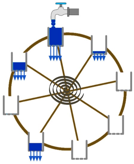
Figure 1. A cartoon of a linear-jerk-controlled chaotic waterwheel. Water inflow fills the water cups, creating a torque that keeps the wheel rotating. At the center of the waterwheel, a controlled spring is designed to control the jerk and avoid (in principle) large pulls.

The waterwheel’s mechanism is simple: water is introduced from the top of the system at a consistent rate. If the flow rate is too slow, the top cups will not receive enough water to overcome friction, and the wheel will remain stationary. However, when the inflow rate increases, the top cup becomes heavy enough to set the wheel in motion. The wheel eventually reaches a stable rotation in either direction because both directions are equally likely, depending on the initial conditions. Interestingly, a further increase in flow rate causes the stable rotation to become chaotic. During this chaotic motion, the wheel rotates in one direction for a few turns before some cups become too full, slowing down or reversing the wheel’s direction. The wheel changes direction erratically, and observers have been known to place small bets on its subsequent turn after a minute.

The equations of motion for the original waterwheel are discussed in Ref. [2] and are derived from two basic principles:

$$\begin{array}{cc}\hfill I{\omega }^{\prime }=\underset{\mathrm{damping}\mathrm{torque}}{\underbrace{-\nu \omega }}+\underset{\mathrm{gravitational}\mathrm{torque}}{\underbrace{gr{\int }_0^{2\pi }m(\theta ,t)sin\theta d\theta }}& (\mathrm{Rigid}-\mathrm{body}\mathrm{motion}\mathrm{of}\mathrm{the}\mathrm{wheel})\end{array}$$

(1)

$$\begin{array}{cc}\hfill \frac{\partial m}{\partial t}=\underset{\mathrm{water}\mathrm{inflow}}{\underbrace{Q}}\underset{\mathrm{water}\mathrm{loss}}{\underbrace{-Km}}\underset{\mathrm{water}\mathrm{transport}}{\underbrace{-\omega \frac{\partial m}{\partial \theta }}}& (\mathrm{Conservation}\mathrm{of}\mathrm{water}),\end{array}$$

(2)

where

• $\theta =$ angle in the lab frame.
• $\omega \left(t\right)={\theta }^{\prime }$, the angular velocity of the wheel.
• $\alpha \left(t\right)={\omega }^{\prime }$, the angular acceleration of the wheel.
• $m(\theta ,t)=$ mass distribution of water at (angular) position $\theta$.
• $Q\left(\theta \right)=$ water inflow rate.
• $r=$ the wheel’s radius.
• $K=$ the amount of mass lost.
• $\nu =$ the viscous damping coefficient.
• $I=$ moment of inertia of the wheel.

As mentioned above, many control systems introduced a jerk-reduction feedback control. In our case, we introduce an additional mechanism into (1),

$$\mathrm{Controlling}\mathrm{torque}:-\lambda {\omega }^{″}\equiv \lambda {\alpha }^{\prime },$$

(3)

where ${\omega }^{″}$ is the angular jerk of the waterwheel. Due to the circular symmetry of the wheel, we can expand

$$m(\theta ,t)=\sum _{n=0}^{\infty }\left[a_n\left(t\right)sinn\theta +b_n\left(t\right)cosn\theta \right].$$

and

$$Q\left(\theta \right)=\sum _{n=0}^{\infty }{q}_{n}cosn\theta .$$

Following the same derivation using amplitude equations, as in Appendix A (similar to the derivation in Ref. [2]), we arrive at:

$$\begin{array}{cc}\hfill & {\alpha }^{\prime }=\left(-\nu \omega +\pi gr{a}_1-I\alpha \right)/\lambda \hfill \\ \hfill & {\omega }^{\prime }=\alpha \hfill \\ \hfill & {a^{\prime }}_1=\omega b_1-K{a}_1\hfill \\ \hfill & {b^{\prime }}_1=-\omega a_1-K{b}_1+q_1.\hfill \end{array}$$

(4)

2.2. Immunology: IL7 Receptor Signaling in T Cells

T-cells play a crucial role in the adaptive immune response of jawed vertebrates. The regulation of T-cell homeostasis is achieved through the secretion and degradation of cytokines, including interleukin 7 (IL7) [18]. Recent studies have suggested that T-cells exhibit elastic-type behavior, which could explain their population-level regulation [19]. This elasticity is a macroscopic property that emerges from the coordinated behavior of individuals rather than from individual agents themselves.

We aim to model the population of T-cells, denoted as x, and the IL7 cytokine, denoted as $h\left(t\right)$, by connecting the dynamics at the receptor level [18] with those at the population level [18,19,20]. Specifically, we propose the following equations:

$$\begin{array}{ccc}\hfill x^{″}& =& -kx-c{x}^{\prime }+\lambda y,\hfill \end{array}$$

(5)

$$\begin{array}{ccc}\hfill y^{\prime }& =& \phi x-\mu xz-\delta y,\hfill \end{array}$$

(6)

$$\begin{array}{ccc}\hfill z^{\prime }& =& \nu xy-\beta z,\hfill \end{array}$$

(7)

Here, k and c represent the T-cell population’s damping coefficient and elastic constant. The parameter $\lambda$ measures the force exerted on the population per unit of interleukin y. The interleukin production rate is $\phi$ per cell, while the interleukin consumption rate is $\mu$ per cell per IL7 receptor, $\rho$. The clearance rate of IL7 due to absorption by other cells (rather than T-cells or dilution in the lymphatic system) is represented by $\delta$. The ligand-induced expression of IL7 receptors per cell is denoted as $\nu$, and the downregulation rate of IL7 receptors at the cell level is represented by $\beta$ [18].

2.3. Ecology: The Evolution of Coexisting Populations

Consider a population of four species in an ecological niche. Mathematically, their dynamics can be modeled using the generalized Lotka–Volterra (gLV) model [8] (or generalizations [9]). According to gLV, the time course of each population follows the first-order system of non-linear equations

$$x_i^{\prime }=r_i{x}_i+\sum _{j=1}^4{\beta }_{ij}{x}_i{x}_j,\forall i=1\dots 4.$$

(8)

In this case, it is often useful to aggregate species based on their role in the ecosystem (predator, prey, …). Also, the relevance of each species is calibrated in proportion, $b_{ij}$, to their diversity. Thus, one can define a meta-population as follows:

$$\begin{array}{ccc}\hfill x_i& =& \sum _{i=1}^4{a}_{ij}{y}_j,\mathrm{and}\mathrm{its}\mathrm{inverse},\hfill \end{array}$$

(9)

$$\begin{array}{ccc}\hfill y_j& =& \sum _{i=1}^4{b}_{ji}{x}_i,\hfill \end{array}$$

(10)

where the matrix $\left[b_{ij}\right]$ is the inverse of $\left[a_{ij}\right]$, namely,

$$\sum _{j=1}^4{a}_{ij}{b}_{jk}={\delta }_{ik},$$

where ${\delta }_{ik}$ is the Kronecker delta function.

Plugging these definitions into (8), we find:

$$y_j^{\prime }=\sum _{k=1}^4\sum _{i=1}^4{b}_{jk}{r}_k{a}_{ki}{y}_i+\sum _{k=1}^4\sum _{i=1}^4{\gamma }_{jki}{y}_k{y}_i,\forall j=1\dots 4.$$

(11)

where ${\gamma }_{jki}$ depends on the matrices a, b, and $\beta$. Without defining a specific problem, it is trivial to see that proper choices of b, $r_i$, and $\beta$ can be mapped into the system of Equation (20) (Lorenz), specifically, choosing ${\gamma }_{1ki}=0$. This might be why chaotic oscillations have been observed in ecological systems [21].

2.4. Rheology

Our final example is the most elaborated one and deserves deeper exposition. Here, we narrow our focus on examining thermosyphon models that involve viscoelastic fluids. This presents some interesting peculiarities that could impact the behavior of a Newtonian fluid, such as water. On one hand, the dynamics exhibit memory, as they depend on past events. On the other hand, small disturbances cause the fluid to act like an elastic solid with a resonant frequency that may eventually become significant.

The simplest method of dealing with viscoelasticity is through the use of the Maxwell constitutive equation [12,22]. Despite being a simplified model, it has been demonstrated to be valid even for complex fluids like blood, in which red blood cells alter their behavior based on concentration and vessel geometry [23]. In this model, both Newton’s law of viscosity and Hooke’s law of elasticity are generalized and supplemented by an evolution equation for the stress tensor, $\mathsf{\Sigma }$. The stress tensor is involved in the conservation of momentum equation.

$$\rho \left(\frac{\partial \mathbf{v}}{\partial t}+\mathbf{v}·\nabla \mathbf{v}\right)=-\nabla p+\nabla ·\mathsf{\Sigma }+\rho \mathbf{g},$$

(12)

Here, p represents the hydrostatic pressure, $\rho$ stands for the material density, and $\mathbf{g}$ denotes the acceleration caused by gravity ($g=9.81$ m/s${}^2$). Additionally, the continuity equation is introduced as a complement to the aforementioned equation, assuming the material to be incompressible (which holds sufficiently true for liquids):

$$\nabla ·\mathbf{v}=0.$$

(13)

In the case of a thin section thermosyphon with a Maxwell fluid, the stress tensor $\mathsf{\Sigma }$ simplifies to a single independent component, denoted as $\tilde{\sigma }$. This component follows the evolution governed by the equation:

$$\frac{\mu }{E}\frac{\partial \tilde{\sigma }}{\partial t}+\tilde{\sigma }=\mu \dot{\gamma },$$

(14)

Here, $\mu$ represents the viscosity of the fluid, E corresponds to Young’s modulus, and $\dot{\gamma }$ is the only non-zero element of the shear strain rate tensor $\dot{\mathsf{\Gamma }}$ (which describes the rate of fluid deformation), defined as

$$\dot{\mathsf{\Gamma }}=\left(\nabla \mathbf{v}+{\left(\nabla \mathbf{v}\right)}^T\right).$$

Under steady flow conditions, Equation (14) reduces to Newton’s law, leading to the well-known Navier–Stokes equation expressed in Equation (12). Additionally, for short time scales when we expect an impulsive response from a resting state, Equation (14) simplifies to Hooke’s law of elasticity.

In order to elucidate the coupling between fluid and thermodynamic mechanisms discussed in Section 1, we shall establish a mathematical framework that encompasses the variables of interest: the velocity v, the temperature distribution T within the fluid, and the concentration S of the solute as it circulates through the loop. The behavior of the solute concentration is governed by transport equations.

$$\begin{array}{ccc}\hfill \rho \left(\frac{\partial T}{\partial t}+\mathbf{v}·\nabla T\right)& =& -\nabla ·{\mathbf{J}}_T+K_T\hfill \end{array}$$

(15)

$$\begin{array}{ccc}\hfill \rho \left(\frac{\partial S}{\partial t}+\mathbf{v}·\nabla S\right)& =& -\nabla ·{\mathbf{J}}_S+K_S\hfill \end{array}$$

(16)

In the given context, ${\mathbf{J}}_{T,S}$ denote the flows or currents of heat and solute concentration, while $K_{T,S}$ represent external sources of temperature or solute concentration. Generally, these terms are determined by constitutive equations that involve linear combinations of gradients of other variables. For example, according to Fourier’s law of heat conduction, ${\mathbf{J}}_T=-\nu \nabla T$; thus, Equation (15) yields the familiar Laplacian term $\nu {\nabla }^{2}T$.

To proceed, we follow the same procedure as in Ref. [24], also summarized in Appendix A, and we arrive at the following equation, which generalizes Equation (2) for a viscoelastic fluid.

$$\rho \frac{\mu }{E}{\left(\frac{d^{2}v}{d{t}^2}\right)}_s+\rho {\left(\frac{dv}{dt}\right)}_s=-\rho gcos\varphi +F_s-\nabla \left(\frac{\partial p}{\partial x}+\frac{\mu }{E}\frac{{\partial }^{2}p}{\partial x\partial t}\right),$$

(17)

where the term $F_s$ represents the component of the wall law force that acts along the pipe (more details on this function are provided below).

Additional physical assumptions, constitutive equations, and nondimensionalization lead to our main system of equations (see Appendix A):

$$\left\{\begin{array}{c}{\displaystyle \epsilon \frac{d^{2}v}{d{t}^2}+\frac{dv}{dt}+G\left(v\right)v=\oint (T(t,x)-S(t,x))f\left(x\right)dx,v\left(0\right)=v_0,\frac{dv}{dt}\left(0\right)=w_0}\\ {\displaystyle \frac{\partial T}{\partial t}+v\frac{\partial T}{\partial x}=h(t,x)+\nu \frac{{\partial }^{2}T}{\partial x^2},T(0,x)=T_0\left(x\right)}\\ {\displaystyle \frac{\partial S}{\partial t}+v\frac{\partial S}{\partial x}=c\frac{{\partial }^{2}S}{\partial x^2}-b\frac{{\partial }^{2}T}{\partial x^2},S(0,x)=S_0\left(x\right)}\end{array}\right.$$

(18)

The expression $h(t,x)+\nu \frac{{\partial }^{2}T}{\partial x^2}$ denotes the heat transfer law along the loop, where $h(t,x)$ is a known function (refer to [25,26]). As stated in the introduction, this study offers an alternative approach to the widely used Newton’s linear cooling model discussed in [13]. Our specific focus lies in investigating a non-Newtonian heat transfer law that takes into account the presence of a viscoelastic fluid.

While previous works, such as [14,15], have employed this heat transfer law in modeling thermosyphons with Newtonian fluids, they did not account for the viscoelastic effects. Hence, our current investigation merges both extensions, addressing the classical thermosyphon problem in a comprehensive manner.

In Appendix A, we provide a detailed analytical study of the system, including the well-posedness of the ODE/PDE model, the existence of a global attractor, and the construction of an inertial manifold. The inertial manifold enables us to describe the system’s asymptotic behavior via a unified and explicitly reduced system of ODEs.

3. Numerical Experiments

This section presents numerical experiments using MATLAB to integrate the differential equations numerically. In particular, we use the solver ode15s for stiff systems.

As shown in Appendix A, we derive the system of equations

$$\left\{\begin{array}{c}\epsilon \dot{w}=2a_1-2d_1-G\left(v\right)v-w\\ \dot{v}=w\\ \dot{a_1}=A-\nu 4{\pi }^2{k}^2{a}_1+2\pi kv{a}_2\\ {\displaystyle \dot{a_2}=B-2\pi v{a}_1-\nu 4{\pi }^2{a}_2}\\ \dot{d_1}=-c4{\pi }^2{d}_1+b4{\pi }^2{a}_1+v2\pi d_2\\ \dot{d_2}=-c4{\pi }^2{d}_2+b4{\pi }^2{a}_1-v2\pi d_1\end{array}\right.$$

(19)

where $(a_1\left(t\right),a_2\left(t\right))$ describe the temperature $T(t,x)$, $(d_1\left(t\right),d_2\left(t\right))$ describe the solute concentrations $S(t,x)$ and $w\left(t\right),andv\left(t\right)$ denotes the acceleration and the velocity of the fluid.

We prove in Appendix A.4 that the asymptotic behavior of the temperature $T(t,x)$ and the solute concentration $S(t,x)$ are given by the coefficients of Fourier expansions $a_k\left(t\right)$ and $d_k\left(t\right)$, respectively, with $k=\pm 1$ for a circular circuit. Moreover, the equation for $k=-1$ is the conjugate of $k=1$, and this is enough to consider $k=1$. Thus, if $b_1$ is the coefficient of the Fourier expansions of the heat flux, we obtain Equation (A72).

Finally, after of change of variables (see Remark A4), in order to simplify the notations, we can omit the subscripts since we only have one coefficient; $a\left(t\right)$ and $d\left(t\right)$ denote the temperature and solute concentrations, respectively. We consider the real and imaginary parts of these coefficients, given by

$$a\left(t\right)=a_1\left(t\right)+i{a}_2\left(t\right),d\left(t\right)=d_1\left(t\right)+i{d}_2\left(t\right)\mathrm{and}{b}_1=A+iB.$$

Notice that if we assume the viscoelastic parameter $\epsilon$, and the Soret diffusion coefficients b and c are zero, we recover the model analyzed in [14] for a Newtonian fluid. Moreover, if we include the Soret effect, but $\epsilon =0$, our model reduces to that in Ref. [15].

Hereafter, we consider the full model (19) (that we refer to as Model M3), a simplified model without the Soret effect (Model M1), and the viscoelastic Lorenz model (Model M2). Although M1 and M2 are intrinsically equivalent, we study this using the traditional parametrization to preserve the familiarity with the Lorenz model in the chaos literature.

Also, as the general model (19) supersedes the other two, and it has a ground physical interpretation, we entitle Section 3.1 and Section 3.3 explicitly in terms of the physical assumptions underlying each model.

3.1. M1 $\left(\right(v\left(t\right),T(t,x))$: Thermodiffusion and Viscoelasticity in a Closed-Loop Thermosyphon without Solute S(t,x)

In this section, we consider a fluid without solute and we analyze and discuss the behavior of the $v\left(t\right)$ and the temperature $T(t,x)$ ( $a_1\left(t\right)$, and $a_2\left(t\right)$) of the fluid, given by the solutions of the following system:

$$\left\{\begin{array}{c}\epsilon \dot{w}=2a_1-G\left(v\right)v-w\\ \dot{v}=w\\ \dot{a_1}=A-\nu 4{\pi }^2{k}^2{a}_1+2\pi kv{a}_2\\ {\displaystyle \dot{a_2}=B-2\pi v{a}_1-\nu 4{\pi }^2{a}_2}\end{array}\right.$$

(20)

We describe the results of numerical experiments that were obtained, considering various parameters of the viscoelastic coefficients.

In the absence of viscoelasticity, the Lorenz-type behavior of the system was observed, see [14]. Therefore, for the numerical simulations, we take the same values of the parameters and the initial conditions as in [14] to explore the effect of viscoelasticity on the chaotic behavior of the system. That is, $A=0,B=30$, and $\nu =0.025$, and the initial conditions, are fixed as $w\left(0\right)=,v\left(0\right)=0, a_1\left(0\right)=-0.1,\mathrm{and}{a}_2\left(0\right)=1.$

We study the behavior of the system upon varying the viscoelastic coefficient $\epsilon$. To assess the effect of viscoelasticity on the system response, we generated a bifurcation diagram to visualize the dynamic behavior of the system. The parameter $\epsilon$ serves as a control variable that represents the degree of viscoelasticity in the system. By varying $\epsilon$ and observing the corresponding peaks of the fluid velocity at large times, we can gain valuable insights into the system’s response under different viscoelastic conditions, see Figure 2.

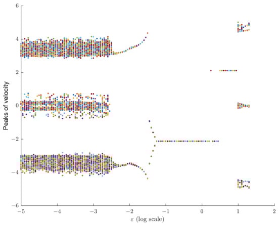
Figure 2. Bifurcation diagram Model M1. We only vary the viscoelastic parameter $\epsilon$ to emphasize the role of elasticity in the chaotic/non-chaotic nature of the solutions. Despite the fact that elasticity is associated with oscillatory motion, we show that new patterns of chaotic behavior arise for large values of $\epsilon$.

Through the analysis of the bifurcation diagram, we can observe that if the parameter value is small, chaos remains as expected. Then, between epsilon ${10}^{-2}$ and ${10}^{-1}$, there seems to be a region of periodicity that transitions into stable behavior between ${10}^{-1}$ and 10. However, the surprising finding is that near 10, the velocity behavior becomes more complex.

Given the multidimensional nature of the system, we plot the velocity in temporal graphs or the impact of the relevant modes of temperature on velocity in phase-space diagrams. During our analysis, we carefully observe significant qualitative changes in the system’s behavior. For low enough values of $\epsilon$, we recover, as expected, Lorenz-type behaviors observed in [14]; see Figure 3. In fact, the system presents chaotic behavior when the value of the viscoelastic component is between ${10}^{-7}$ and ${10}^{-3}$.

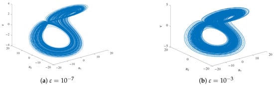
Figure 3. Temperature velocity phase diagram $(a_1,a_2,v)$ for Model M1.

By increasing the viscoelastic coefficient, a significant alteration in the system’s behavior becomes apparent. As the coefficient increases within the range of ${10}^{-3}$ to ${10}^{-2}$, the system’s behavior gradually undergoes a transformation, eventually transitioning into a periodic pattern. Observe the emergence of periodic behavior in the velocity at ${10}^{-2}$, Figure 4, and observe that the phase diagram has simplified for $\epsilon ={10}^{-2.4}$, Figure 5.

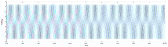
Figure 4. Example of velocity evolution for $\epsilon ={10}^{-2}$ for Model M1.

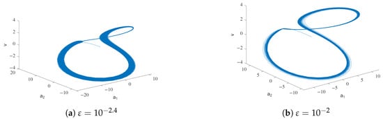
Figure 5. Temperature velocity phase diagram $(a_1,a_2,v)$ for Model M1.

Beyond ${10}^{-2}$, the system begins to stabilize. For instance, for $\epsilon ={10}^{-1}$, after a transition, the system has stable behavior. Notice that, in this case, equilibrium is reached. This behavior holds until $\epsilon =10$. However, it is important to note that the transition becomes more complex as $\epsilon$ is larger; see Figure 6.

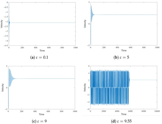
Figure 6. Comparison of four velocity time-courses for different values of $\epsilon$ and fixing the rest of the parameters of Model M1. Note how small changes in $\epsilon$ between panels (c,d) also induce transient chaotic behavior followed by stability at a fixed point.

Corroborating what was observed in the phase diagram, as the value of $\epsilon$ approaches 10, the system shows a tendency to exhibit more complex behaviors. This observation becomes evident when $\epsilon$ varies between 10 and 12. Surprisingly, within this range, the system reverts back to displaying chaotic behavior; see Figure 7.

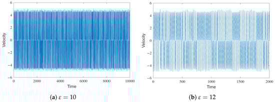
Figure 7. Velocity evolution on time.

Finally, when $\epsilon$ goes beyond 12, the system stabilizes. First, quasi-periodic behavior is observed, and then, as $\epsilon$ is large enough, periodic behavior is found; see Figure 8.

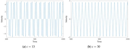
Figure 8. Velocity evolution on time.

In summary, the effect of the viscoelastic parameter $\epsilon$ on chaos is far from trivial. For large values, it tends to remove chaos but, as shown in Figure 2, there are regions where chaos reappears. To study this more systematically, in the discussion section, we display the maximum value of the Lyapunov exponent for different values of $\epsilon$.

3.2. M2 General Lorenz System: Considering the Viscoelastic Fluid

For the thermosyphon model without viscoelasticity, $\epsilon =0$ in (20), equivalence with the classical Lorenz equations was shown, see [14]. The authors performed some changes of variables to prove that the three-dimensional model of the thermosyphon corresponded exactly to the Lorenz system in the case of linear friction. Analogously, performing the same changes of variables as in [14], we obtain from (20) the following system:

$$\left\{\begin{array}{c}\epsilon w^{\prime }=\sigma (y-x)-w\\ x^{\prime }=w\\ y^{\prime }=x·(\rho -z)-y\\ {\displaystyle z^{\prime }=xy-\beta z.}\end{array}\right.$$

(21)

Observe that if the parameter $\epsilon$ is zero in the previous model, we recover the classical Lorenz system:

$$\left\{\begin{array}{c}{x}^{\prime }=\sigma (y-x)\\ y^{\prime }=x·(\rho -z)-y\\ {\displaystyle z^{\prime }=xy-\beta z.}\end{array}\right.$$

(22)

We are interested in analyzing how the parameter $\epsilon$ variation affects the Lorenz system’s chaotic regime. Therefore, taking the typical parameters that cause chaos in the classical Lorenz system, we analyze and discuss the system’s behavior for different parameters of the viscoelastic coefficients.

Therefore, we consider $\sigma =10,\beta =\frac{8}{3}$, and $\rho =28$, and initial conditions are fixed as $w\left(0\right)=0,x\left(0\right)=1,y\left(0\right)=1$ and $z\left(0\right)=0$.

Following the analysis conducted in the previous model, we first present the bifurcation diagram to understand the system’s behavior, as we vary the parameter $\epsilon$, see Figure 9.

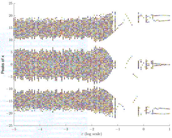
Figure 9. Bifurcation diagram, Model M2, compared with that in Figure 2. Again, elasticity does not mean periodic behavior; rather, new complex regions of chaotic-stable transitions emerge.

Similar to what occurred in the previous model, starting from chaos, when the viscoelasticity is sufficiently small, chaotic behavior persists. However, when $\epsilon$ reaches a value of ${10}^{-1}$, a predictable behavior emerges. It is worth noting that near $\epsilon =1$, small regions with more complex behaviors appear, which require further detailed analyses.

To accomplish this, we will plot the phase diagram of $(x,y,z)$ for notable parameter values where the behavior changes. The chaotic behavior of the system is observed for small enough $\epsilon$. Specifically, the classical Lorenz-type behavior remains from ${10}^{-7}$ to ${10}^{-2}$; see Figure 10.

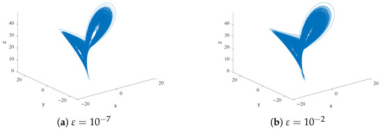
Figure 10. Phase diagram $(x,y,z)$ for Model M2.

At values below $\epsilon =0.1$, the system exhibits chaotic behavior. However, when $\epsilon =0.1$ is reached, the system transitions towards periodic behavior. Remarkably, this periodic behavior persists until $\epsilon =1$, but at $\epsilon =0.1$, the system begins to change from periodic behavior. The system preserves this periodic behavior until $\epsilon =1$; see Figure 11.

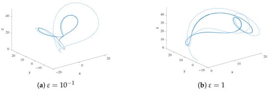
Figure 11. Phase diagram $(x,y,z)$ for Model M2.

Similar to the previous model, we have identified parameter values of epsilon that induce chaos from the initial periodic behavior of the system. In particular, for parameter $\epsilon$ values between $1.2$ and $1.5$, the system reverts back to chaotic behavior Figure 12.

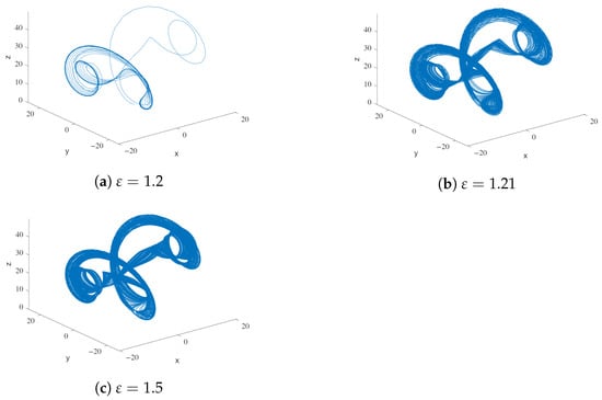
Figure 12. Phase diagram $(x,y,z)$ for Model M2.

After $\epsilon =1.5$ the behavior changes drastically again. For $\epsilon =1.6$, the solutions present a periodic behavior. Finally, the behavior becomes stable for larger values of the parameter $\epsilon$.

As mentioned above, the Lorenz model is a paradigmatic case of a simple model displaying a route to chaos. To illustrate this, we show four bifurcation diagrams for the Lorenz parameter $\rho$ in Figure 13. Note that, for small values of the viscoelastic parameter $\epsilon$, the two bifurcation diagrams are almost identical (so the chaotic patterns are preserved even though $\epsilon \to 0$ is a singular perturbation). Interestingly, larger values stretch the bifurcation pattern and create new stability gaps.

Figure 13. Comparison of bifurcation diagrams for the Lorenz parameter $\rho$ with and without elasticity. The Lorenz system, (22), is represented with blue dots, and the system (21) is represented with green dots.

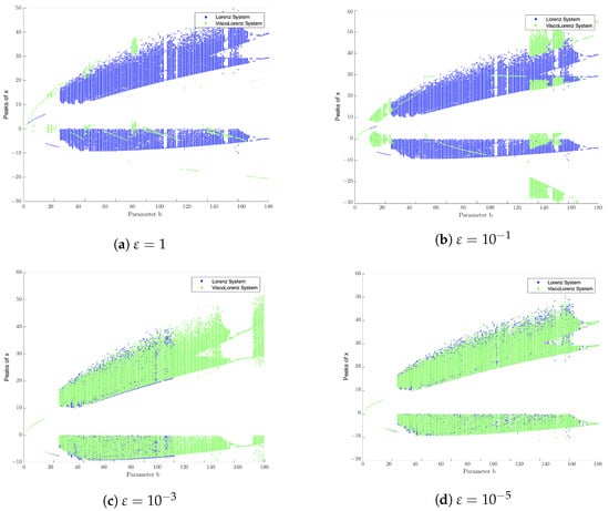
This similarity between bifurcation diagrams is best quantified in Figure 18 (red line). For values of $\epsilon \le {10}^{-1.4}$, the Lyapunov exponent is the same as the original Lorenz system’s. It is also worth noting that the appearance of chaos is intermittent for larger values, as seen in Figure 9.

3.3. M3 $\left(v\right(t),T(t,x),S(t,x\left)\right)$: General Model (19)

In this subsection, we analyze the influence of viscoelasticity in the general case where a binary fluid is considered, this is when we consider a solute (as water and antifreeze), and we study the evolution of the velocity $v\left(t\right)$, the temperature $T(t,x)$ of the fluid (given by $a_1\left(t\right),a_2\left(t\right))$ and the solute concentrated $S(t,x)$ (given by $d_1\left(t\right),d_2\left(t\right))$, see (19).

We are going to proceed as in the previous cases. We will assume the values calculated [15] in order to obtain chaos, and then, we discuss the behavior of the new system depending on the value of the viscoelasticity $\epsilon$. Therefore, we take $A=0,$ $B=30,$ $\nu =0.025,c=0.001$ and $b={10}^{-3}$. Moreover, we consider the initial conditions $w\left(0\right)=0,$ $v\left(0\right)=0,a_1\left(0\right)=-0.1,a_2\left(0\right)=1,d_1\left(0\right)=0.01,d_2\left(0\right)=1$.

First, to understand the system’s behavior globally, we plotted the bifurcation velocity diagram for large time values; see Figure 14.

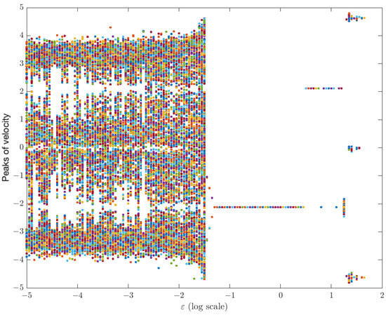
Figure 14. Bifurcation diagram for Model M3. As discussed for models M1 and M2, the role of elasticity is not to force oscillations (or resonance) but to change the chaotic behavior dramatically.

Repeating the pattern observed in previous models, for small parameter values, chaotic behavior is preserved, and as the parameter representing viscoelasticity increases, chaos disappears. However, what is interesting is that for values greater than 10 in the diagram, more complex behaviors are once again observed.

To further validate the conclusions derived from the bifurcation diagram, we will graph the velocity and the temperature phase diagram for specific values of the parameter epsilon that are deemed relevant. First, we confirm the intuitive idea that while the viscoelastic coefficient is small, the behavior remains chaotic. In particular, from $\epsilon ={10}^{-7}$ to $\epsilon ={10}^{-2}$ chaotic behavior of the system is observed; see Figure 15.

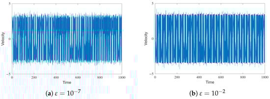
Figure 15. Velocity evolution for Model M3.

However, once $\epsilon$ exceeds ${10}^{-2}$, the system stabilizes rapidly, transitioning from chaotic behavior to equilibrium. Specifically, from $\epsilon ={10}^{-2}$ to $\epsilon ={10}^{-1}$, the system demonstrates periodic behavior; see Figure 16. At $\epsilon ={10}^{-1.2}$, the velocity initially undergoes a complex transition but eventually converges to equilibrium. This stabilizing effect continues to manifest with varying degrees of complexity until reaching $\epsilon =10$.

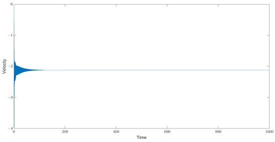
Figure 16. Velocity evolution for $\epsilon ={10}^{-1}$ for Model M3.

For values close to (but greater than) $\epsilon =10$, the behavior of the solutions becomes more complex. First, we obtain periodic behavior, $\epsilon =12$, then quasiperiodic behavior, and chaos from $\epsilon =14$; see Figure 17. Beyond $\epsilon =15$, the system tends to stabilize. Sometimes the system presents periodic behavior, $\epsilon =15$ or $\epsilon =20$, but other times, it converges to equilibrium. For instance, $\epsilon =21$ or 25. As discussed before, the maximum Lyapunov exponent allows to explain this non-monotonic effect of the viscoelastic parameters, as shown in Figure 18.

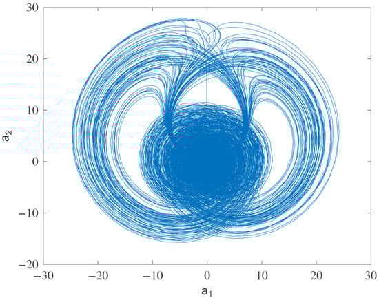
Figure 17. Temperature phase diagram for $\epsilon =14$.

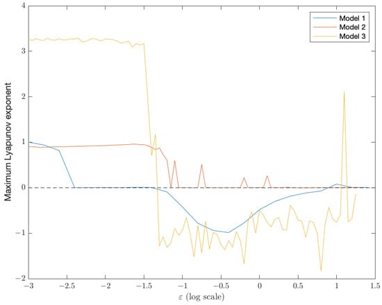
Figure 18. Maximum Lyapunov Exponent. This diagram summarizes the main idea of the work: elasticity is a non-trivial contributor to the emergence or disappearance of chaotic behavior.

4. Discussion

Through our study of three chaotic systems, it is clear that the interaction of viscoelasticity can lead to intricate nonlinear and chaotic behaviors. As a result, drawing conclusions that are not specific to the studied system can be challenging. However, our article provides general insights into all three models based on a thorough analysis of numerical simulations.

For example, while chaos has been observed in ecological systems, our research reveals that this is not contradictory but rather a natural outcome of the Lotka–Volterra model’s inherent structure.

Traditionally, elasticity is linked to phenomena such as oscillations or resonance. However, our study demonstrates that the interplay between elasticity and other model features is more complex, resulting in complex interactions that preserve, modify, and generate novel chaotic regimes.

The intricacies resulting from the interaction of viscoelasticity are evident in the analysis of the three chaotic systems, see Table 1. As such, generalizing results beyond the specific studied systems can pose challenges. Nevertheless, our article provides comprehensive insights into all three models through detailed numerical simulations.

Table 1. Categorization of Models Based on the viscoelastic parameter $\epsilon$. For the sake of simplicity, we group stable and oscillatory behaviors under the label non-chaotic.

Model	Chaos	Non-Chaotic	Chaos	Non-Chaotic
M1	${10}^{-7}<\epsilon <{10}^{-3}$	${10}^{-3}<\epsilon <10$	$10<\epsilon <12$	$12<\epsilon$
M2	${10}^{-7}<\epsilon <{10}^{-2}$	${10}^{-1}<\epsilon <1$	$1.2<\epsilon <1.5$	$\epsilon >1.5$
M3	${10}^{-7}<\epsilon <{10}^{-2}$	${10}^{-2}<\epsilon <12$	$14<\epsilon <15$	$\epsilon >15$

To summarize the behavior of models M1–M3, Figure 18 showcases the maximum Lyapunov exponent, which exhibits a fascinating pattern in the three systems as the viscoelasticity-affecting parameter increases. As viscoelasticity increases, we observe transitions from chaos to predictable long-term behaviors, like equilibria, periodicity, or quasi-periodicity. However, increasing the viscoelastic parameter can reintroduce chaos, highlighting the captivating nature of these systems, wherein changes in the viscoelastic parameter lead to transitions between ordered and chaotic dynamics.

5. Conclusions

This research delves into the role of elasticity in chaotic systems by examining four different models from various fields, such as mechanics, immunology, ecology, and rheology. Through numerical simulations, we discovered that elasticity has a significant impact on the chaotic behavior of these systems, which we refer to as elastic-Lorenz equations. Our study provides insight into the importance of elasticity in chaotic systems and sparks new areas of research.

The implications of our findings are far-reaching. For example, in immunology, where chaos plays a significant role in the behavior of the immune system, understanding the effects of elasticity on chaotic dynamics could be crucial in treating diseases. Our research also has potential applications in rheology, which studies the flow of matter and is vital in many industrial processes. Additionally, our discoveries shed light on complex systems, such as financial markets and ecosystems, where chaotic behavior is prevalent.

Furthermore, our research suggests potential extensions. We used the basic Maxwell model of viscoelasticity, but exploring linear and non-linear generalizations of the constitutive equation could reveal new and exciting phenomena. Another potential extension is the use of time-fractional models, which have successfully modeled viscoelastic materials. As our elasticity-driven models contain both the first and second derivatives of velocity, we hope that further developments in the field will result from our findings.

Appendix A.1. Well-Posedness and Boundedness: Global Attractor

For completeness, we include the details of well-posedness and boundedness for the present model as it requires specific work, although the techniques used are similar to those in Refs. [28,29].

In this context, we enforce the condition that the thermal diffusivity $\nu \ge 0$ maintains physical consistency. The system of Equation (18) represents an ODE/PDE system governing the evolution of the observables v, T, and S. The solute concentration $S(t,x)$ adheres to a solute diffusivity $c>0$ and a positive Soret coefficient b, similar to previous models for binary fluids, like in [6,15,30].

In subsequent discussions, we utilize the notation $\oint ·dx={\int }_0^1·dx$ for integration along a closed circuit path, which can be associated with integration over periodic functions with a period of 1. The function f in the equation characterizes the loop’s geometry and gravitational forces [24,27], where $\oint f\left(x\right)dx=0$, since the integral of $f\left(x\right)=cos\varphi \left(x\right)$ over a closed loop yields zero.

The parameter $\epsilon$ in Equation (18) represents the non-dimensional form of $\mu /E$, with time units. Roughly, $\epsilon$ determines the (non-dimensional) timescale for the material to transition from an elastic to a fluid-like behavior.

We assume that the friction law $G\left(v\right)$ at the inner wall of the loop is positive and remains bounded away from zero. Previous works have considered $G\left(v\right)$ as a constant for linear friction [27] (Stokes flow) or $\left|v\right|$ for quadratic friction [25,26]. A more general form of $G\left(v\right)$ is given by $\tilde{g}\left(Re\right)\left|v\right|$, where $Re=\rho vL/\mu$ is the Reynolds number, and $\tilde{g}$ is a function of $Re$. Here, we consider a general function of the velocity, assumed to be large [31,32]. The functions G, f, and l incorporate relevant physical constants of the model, such as the cross-sectional area D, the length of the loop L, and the Prandtl, Rayleigh, or Reynolds numbers. We require G and l to be continuous functions satisfying $G\left(v\right)\ge G_0>0$ and $l\left(v\right)\ge l_0>0$, where $G_0$ and $l_0$ are positive constants. Additionally, we impose further constraints on G in Equation (A23), mandating G to be a nonlinear friction function, such that there exists a constant $h_0\ge 0$, satisfying the following:

$$\underset{s\to \infty }{lim\; sup}\frac{|G^{\prime }\left(s\right)|}{G\left(s\right)}=0\mathrm{and}\underset{s\to \infty }{lim\; sup}\frac{|s{G}^{\prime }\left(s\right)|}{G\left(s\right)}\le h_0.$$

We will introduce some function spaces that will be used to study the existence of solutions of (18). Let $\mathsf{\Omega }=(0,1)$ and consider the spaces

$$L_{per}^2\left(\mathsf{\Omega }\right)=\{u\in L_{loc}^2\left(IR\right),u(x+1)=u\left(x\right)a.e.x\in IR\},H_{per}^m\left(\mathsf{\Omega }\right)=H_{loc}^m\left(IR\right)\cap L_{per}^2\left(\mathsf{\Omega }\right)$$

(A4)

where $m\in IN\cup \left\{0\right\}$, and $u\in L_{loc}^2\left(IR\right)$ (or $H_{loc}^m\left(IR\right)$) if for every open set $\omega \subset \subset IR$ one has $u\in L_{loc}^2\left(\omega \right)$ (or $H_{loc}^m\left(\omega \right)$, respectively). Finally, we consider functions with zero average, and we denote by the following:

$$\begin{array}{c}\hfill {\dot{L}}_{per}^2(0,1)=\{u\in L_{loc}^2\left(IR\right),u(x+1)=u\left(x\right)a.e.,\oint u\left(x\right)dx=0\},\end{array}$$

(A5)

$$\begin{array}{c}\hfill {\dot{H}}_{per}^m(0,1)=H_{loc}^m\left(IR\right)\cap {\dot{L}}_{per}^2(0,1).\end{array}$$

(A6)

Appendix A.2. Existence and Uniqueness of Solutions

In this section, we demonstrate the presence and singularity of solutions for the thermosyphon model (18), where f and h belong to ${\dot{L}}_{per}^2(0,1)$, $T_0$ is in ${\dot{H}}_{per}^1(0,1)$, and $S_0$ is in ${\dot{L}}_{per}^2(0,1)$. Here, ${\dot{L}}_{per}^2(0,1)$ and ${\dot{H}}_{per}^1(0,1)$ are defined by (A5). It should be noted that the term dot indicates functions that have zero averages and not the time derivatives of the functions. To begin with, we choose this framework by observing that for $\nu >0$, integrating the temperature equation along the loop, while considering the periodicity of T, we have the following:

$\oint \frac{\partial T}{\partial x}dx=\oint \frac{{\partial }^{2}T}{\partial x^2}dx=0,$ and $\frac{d}{dt}\oint T(t,x)dx=(\oint h(t,x).$

Next, if $h(t,x)=h\left(x\right)$, we have $\oint T(t,x)dx=\oint T_0\left(x\right)dx+t\oint h\left(x\right)dx$. Therefore, the temperature is unbounded, as $t\to \infty$, unless $\oint h\left(x\right)dx=0$. However, taking $\tau (t,x)=T(t,x)-\oint T(t,x)dx$ and $h\ast =h-\oint h\left(x\right)dx$ reduces to the case $\oint T(t,x)dx=\oint T_0\left(x\right)dx+t\oint h\left(x\right)dx=0$, since $\tau (t,x)$ would satisfy

$$\frac{\partial \tau }{\partial t}+v\frac{\partial \tau }{\partial x}=h^{*}(t,x)+\nu \frac{{\partial }^2\tau }{\partial x^2},\tau (0,x)={\tau }_0\left(x\right)=T_0\left(x\right)-\oint T_0\left(x\right)dx.$$

Additionally, if we integrate the equation for the solute concentration along the loop and take into account the periodicity of S, we obtain the conditions $\oint \frac{\partial S}{\partial x}dx=\oint \frac{{\partial }^{2}S}{\partial x^2}dx=0$ and $\frac{d}{dt}(\oint S(t,x)dx)=0.$ Since $\oint S(t,x)dx$ is constant, it means that the solute $\oint S(t,x)=\oint S_0\left(x\right)$ for all t.

Let $\sigma (t,x)=S(t,x)-\oint S_0\left(x\right)dx$ (not to be confused with the stress component $\tilde{\sigma }$). Then, from the third equation of system (18), $\sigma$ satisfies the equation:

$$\frac{\partial \sigma }{\partial t}+v\frac{\partial \sigma }{\partial x}=c\frac{{\partial }^2\sigma }{\partial x^2}-b\frac{{\partial }^2\tau }{\partial x^2},\sigma (0,x)={\sigma }_0\left(x\right).$$

Finally, since $\oint f\left(x\right)dx=0$, we have $\oint \left(T\right(t,x)-S(t,x\left)\right)f\left(x\right)dx=\oint \left(\tau \right(t,x)-$ $\sigma (t,x)\left)f\right(x)dx$, and the equation for v is

$$\epsilon \frac{d^{2}v}{d{t}^2}+\frac{dv}{dt}+G\left(v\right)v=\oint (\tau (t,x)-\sigma (t,x))f\left(x\right)dx,v\left(0\right)=v_0,\frac{dv}{dt}\left(0\right)=w_0.$$

Therefore, $(v,\tau ,\sigma )$ satisfies system (18) with ${\tau }_0,{\sigma }_0,h^{*}$ replacing $T_0,S_0,h$, respectively, and $\oint f\left(x\right)dx=\oint {\tau }_0\left(x\right)dx=\oint {\sigma }_0\left(x\right)dx=\oint h^{*}dx=0$ and $\oint T(t,x)dx=\oint S(t,x)dx=0$ for all $t\ge 0.$ From now on, we consider all the functions of system (18) to have zero average.

Furthermore, since $\nu ,c>0$, the operators $\nu A=-\nu \frac{{\partial }^2}{\partial x^2}$ and $cA=-c\frac{{\partial }^2}{\partial x^2}$, along with periodic boundary conditions, are unbounded, self-adjoint operators with a compact resolvent in $L_{per}^2(0,1)$, which are positive when restricted to the space of zero average functions in ${\dot{L}}_{per}^2(0,1)$. Moreover, the equations for the temperature T and the solute concentration S in (18) are parabolic types for $\nu ,c>0.$

We express system (18) as the following evolution system for acceleration, velocity, temperature, and solute concentrations:

$$\left\{\begin{array}{ccc}{\displaystyle \frac{dw}{dt}+\frac{1}{\epsilon }w}& =\hfill & {\displaystyle -\frac{1}{\epsilon }G\left(v\right)v+\frac{1}{\epsilon }\oint (T(t,x)-S(t,x))f\left(x\right)dx,w\left(0\right)=w_0}\hfill \\ \frac{dv}{dt}& -w=\hfill & 0,v\left(0\right)=v_0\hfill \\ {\displaystyle \frac{\partial T}{\partial t}-\nu \frac{{\partial }^{2}T}{\partial x^2}}& =\hfill & -v\frac{\partial T}{\partial x}+h(t,x),T(0,x)=T_0\left(x\right)\hfill \\ {\displaystyle \frac{\partial S}{\partial t}-c\frac{{\partial }^{2}S}{\partial x^2}}& =\hfill & -v\frac{\partial S}{\partial x}-b\frac{{\partial }^{2}T}{\partial x^2},S(0,x)=S_0\left(x\right).\hfill \end{array}\right.$$

(A7)

That is:

$$\frac{d}{dt}\left(\begin{array}{c}w\hfill \\ v\hfill \\ T\hfill \\ S\hfill \end{array}\right)+\left(\begin{array}{cccc}\frac{1}{\epsilon }& 0& 0& 0\\ -1& 0& 0& 0\\ 0& 0& -\nu \frac{{\partial }^2}{\partial x^2}& 0\\ 0& 0& 0& -c\frac{{\partial }^2}{\partial x^2}\end{array}\right)\left(\begin{array}{c}w\hfill \\ v\hfill \\ T\hfill \\ S\hfill \end{array}\right)=\left(\begin{array}{cc}{F}_1(w,v,T,S)\hfill & \\ F_2(w,v,T,S)\hfill & \\ F_3(w,v,T,S)\hfill & \\ F_4(w,v,T,S)\hfill \end{array}\right)$$

(A8)

with

$$\begin{array}{c}\hfill F_1(w,v,T,S)=-\frac{1}{\epsilon }G\left(v\right)v+\frac{1}{\epsilon }\oint (T(t,x)-S(t,x))f\left(x\right)dx,\end{array}$$

(A9)

$$\begin{array}{c}\hfill F_2(w,v,T,S)=0,\end{array}$$

(A10)

$$\begin{array}{c}\hfill F_3(w,v,T,S)=-v\frac{\partial T}{\partial x}+h(t,x),\end{array}$$

(A11)

$$\begin{array}{c}\hfill F_4(w,v,T,S)=-v\frac{\partial S}{\partial x}-b\frac{{\partial }^{2}T}{\partial x^2}\end{array}$$

(A12)

and initial data $\left(\begin{array}{c}w\hfill \\ v\hfill \\ T\hfill \\ S\hfill \end{array}\right)\left(0\right)=\left(\begin{array}{c}{w}_0\hfill \\ v_0\hfill \\ T_0\hfill \\ S_0\hfill \end{array}\right)$.

The operator $B=\left(\begin{array}{cccc}\frac{1}{\epsilon }& 0& 0& 0\\ -1& 0& 0& 0\\ 0& 0& -\nu \frac{{\partial }^2}{\partial x^2}& 0\\ 0& 0& 0& -c\frac{{\partial }^2}{\partial x^2}\end{array}\right)$ is a sectorial operator in $\mathcal{Y}=I{R}^2\times {\dot{H}}_{per}^1(0,1)\times {\dot{L}}_{per}^2(0,1)$ with domain $D\left(B\right)=I{R}^2\times {\dot{H}}_{per}^3(0,1)\times {\dot{H}}_{per}^2(0,1)$ and has a compact resolvent, see Equation (A5).

Using the results and techniques in the sectorial operator of [33] to prove the existence of solutions of the system, we have Theorem A1.

Theorem A1. 

We assume that $H\left(r\right)=rG\left(r\right)$ is locally Lipschitz, $f,h\left(t\right)\in {\dot{L}}_{per}^2(0,1)$, $G\left(v\right)\ge G_0>0$. Then, given $(w_0,v_0,T_0,S_0)\in \mathcal{Y}=I{R}^2\times {\dot{H}}_{per}^1(0,1)\times {\dot{L}}_{per}^2(0,1)$, there exists a unique solution of (18), satisfying

$$(w,v,T,S)\in C([0,\infty ),\mathcal{Y})\cap C(0,\infty ,I{R}^2\times {\dot{H}}_{per}^3(0,1)\times {\dot{H}}_{per}^2(0,1)),$$

$$\left(\frac{dw}{dt},\frac{dv}{dt},\frac{\partial T}{\partial t},\frac{\partial S}{\partial t}\right)\in C(0,\infty ,I{R}^2\times {\dot{H}}_{per}^{3-\delta }(0,1)\times {\dot{H}}_{per}^{2-\delta }(0,1)),$$

for every $\delta >0.$ In particular, (A7) defines a nonlinear semigroup, $S^{*}\left(t\right)$ in $\mathcal{Y}=I{R}^2\times {\dot{H}}_{per}^1(0,1)\times {\dot{L}}_{per}^2(0,1),$ with $S^{*}\left(t\right)(w_0,v_0,T_0,S_0)=(w\left(t\right),v\left(t\right),T(t,x),S(t,x))$.

Proof. 

In order to prove this, we cover several steps:

Step (i). We prove the local existence and regularity. This follows easily from the variation of the constants formula as presented in [33]. In order to prove this, we write the system as (A8), and we have:

$$U_t+BU=F\left(U\right),withU=\left(\begin{array}{c}w\hfill \\ v\hfill \\ T\hfill \\ S\hfill \end{array}\right),$$

$$B=\left(\begin{array}{cccc}\frac{1}{\epsilon }& 0& 0& 0\\ -1& 0& 0& 0\\ 0& 0& -\nu \frac{{\partial }^2}{\partial x^2}& 0\\ 0& 0& 0& -c\frac{{\partial }^2}{\partial x^2}\end{array}\right),$$

$$F=\left(\begin{array}{c}{F}_1\hfill \\ F_2\hfill \\ F_3\hfill \\ F_4\hfill \end{array}\right)$$

where the operator B is a sectorial operator in $\mathcal{Y}=I{R}^2\times {\dot{H}}_{per}^1(0,1)\times {\dot{L}}_{per}^2(0,1)$ with domain $D\left(B\right)=I{R}^2\times {\dot{H}}_{per}^3(0,1)\times {\dot{H}}_{per}^2(0,1)$, and has a compact resolvent. In this context, operator $A=-\frac{{\partial }^2}{\partial x^2}$ must be understood in the variational sense, i.e., for every $T,\phi \in {\dot{H}}_{per}^1(0,1)$,

$$⟨A\left(T\right),\phi ⟩=\oint \frac{\partial T}{\partial x}\frac{\partial \phi }{\partial x}dx$$

and ${\dot{L}}_{per}^2(0,1)$ coincides with the fractional space of exponent $\frac{1}{2}$, as in [33]. We denote ${\dot{H}}_{per}^{-1}(0,1)$ as the dual space and $\parallel .\parallel$ as the norm on the space ${\dot{L}}_{per}^2(0,1)$. If we prove that the nonlinearity $F:\mathcal{Y}=I{R}^2\times {\dot{H}}_{per}^1(0,1)\times {\dot{L}}_{per}^2(0,1)\mapsto {\mathcal{Y}}^{-\frac{1}{2}}=I{R}^2\times {\dot{L}}_{per}^2(0,1)\times {\dot{H}}_{per}^{-1}(0,1)$ is well defined, Lipschitz, and bounded on bounded sets, we obtain the local existence for the initial data in $\mathcal{Y}=I{R}^2\times {\dot{H}}_{per}^1(0,1)\times {\dot{L}}_{per}^2(0,1)$.

Using $H\left(v\right)\equiv G\left(v\right)v$ as a locally Lipschitz function, with $f,h\left(t\right)\in {\dot{L}}_{per}^2(0,1)$, we can follow the approach in [28], and we will prove the nonlinear terms, $F_{1\dots 4}$ in Equations (A9)–(A12), satisfying $F_1:I{R}^2\times {\dot{L}}_{per}^2(0,1)\times {\dot{L}}_{per}^2(0,1)\mapsto IR$, $F_2:I{R}^2\times {\dot{H}}_{per}^1(0,1)\times {\dot{L}}_{per}^2(0,1)\mapsto IR,$ $F_3:I{R}^2\times {\dot{H}}_{per}^1(0,1)\times {\dot{L}}_{per}^2(0,1)\mapsto {\dot{L}}_{per}^2(0,1)$ and $F_4:I{R}^2\times {\dot{H}}_{per}^1(0,1)\times {\dot{L}}_{per}^2(0,1)\mapsto {\dot{H}}_{per}^{-1}(0,1)$; that is, $F:\mathcal{Y}\mapsto {\mathcal{Y}}^{-\frac{1}{2}}$ is well defined, Lipschitz, and bounded on bounded sets.

For $F_3$, in this case, we have that

$$\parallel F_3(w_1,v_1,T_1,S_1)-F_3(w_2,v_2,T_2,S_2)\parallel =\parallel -v_1{\left(T_1\right)}_x+v_2{\left(T_2\right)}_x\parallel \le$$

$$\le \parallel (v_2-v_1)\left(T_1\right)x\parallel +\parallel v_2{\left((T_2-T_1)\right)}_x\parallel \le$$

$$\le \parallel v_2-v_1{\parallel }_{\infty }\parallel T_1{\left(t\right)\parallel }_{{\dot{H}}_{per}^1}+\parallel v_2{\parallel }_{\infty }{\parallel T_2-T_1\left(t\right)\parallel }_{{\dot{H}}_{per}^1}\le$$

$$\le C\left(\parallel v_2-v_1{\parallel }_{\infty }+{\parallel T_2-T_1\left(t\right)\parallel }_{{\dot{H}}_{per}^1}\right).$$

In this way, $F_3$ is locally Lipschitz and bounded on bounded sets.

Applying the techniques of the variation of constants formula from [33], we obtain the unique local solution $(w,v,T,S)\in C([0,t^{*}],\mathcal{Y})$ (with a suitable $t^{*}>0$) of (A7), which is given by

$$\begin{array}{cc}w\left(t\right)=\hfill & w_0{e}^{-\frac{1}{\epsilon }t}-\frac{1}{\epsilon }{\int }_0^t{e}^{-\frac{1}{\epsilon }(t-r)}H\left(r\right)dr+\hfill \\ \hfill & +\frac{1}{\epsilon }{\int }_0^t\left[\oint \left(T\right(r,x)-S(r,x\left)\right)f\left(x\right)dx\right]e^{-\frac{1}{\epsilon }(t-r)}dr\hfill \end{array}$$

(A13)

with $H\left(r\right)=G\left(v\right(r\left)\right)v\left(r\right)$.

$$v\left(t\right)=v_0+{\int }_0^{t}w\left(r\right)dr$$

(A14)

$$\begin{array}{ccc}\hfill T(t,x)& =& e^{-\nu At}{T}_0\left(x\right)+{\int }_0^t{e}^{-\nu A(t-r)}h(x,r)]dr\hfill \\ & & -{\int }_0^t{e}^{-\nu A(t-r)}v\left(r\right)\frac{\partial T(r,x)}{\partial x}dr,\hfill \end{array}$$

(A15)

$$S(t,x)=e^{-cAt}{S}_0\left(x\right)+{\int }_0^t{e}^{-cA(t-r)}[-v\left(r\right)\frac{\partial S}{\partial x}\left(r\right)-b\frac{{\partial }^{2}T}{\partial x^2}\left(r\right)]dr.$$

(A16)

where $(w,v,T,S)\in C([0,t^{*}],\mathcal{Y}=I{R}^2\times {\dot{H}}_{per}^1(0,1)\times {\dot{L}}_{per}^2(0,1))$ and using the results from [33], (the smoothing effect of the equations with the bootstrapping method), we obtain the regularity of solutions.

Step (ii). To prove global existence, we must show that the solutions are bounded in the $\mathcal{Y}=I{R}^2\times {\dot{H}}_{per}^1(0,1)\times {\dot{L}}_{per}^2(0,1)$ norm on finite time intervals, and using the nonlinearity of $F,$ maps bounded on bounded sets, we can conclude.

Part I: We study the norm of temperature, T.

To prove that the norm of T is bounded on finite time, we multiply the equation for the temperature by T in ${\dot{L}}_{per}^2(0,1).$ Then, integrating by parts, we obtain:

$$\frac{1}{2}\frac{d}{dt}{\parallel T\parallel }^2+\nu {\parallel \frac{\partial T}{\partial x}\parallel }^2=\oint h(t,x)T(t,x)dx$$

since $\oint T(t,x)\frac{\partial T}{\partial x}dx=\frac{1}{2}\oint \frac{\partial }{\partial x}\left(T^2\right)dx=0$.

By using Cauchy–Schwartz and Young inequalities, as well as the Poincaré inequality for functions of zero average, since $\oint T(t,x)dx=0,$, and as ${\pi }^2$ is the first nonzero eigenvalue of $A=-\frac{{\partial }^2}{\partial x^2}$ in ${\dot{L}}_{per}^2(0,1)$, we obtain

$$\frac{1}{2}\frac{d}{dt}{\parallel T\parallel }^2+\nu {\pi }^2{\parallel T\parallel }^2\le \frac{1}{4\delta }{\parallel h\left(t\right)\parallel }^2+\delta {\parallel T\parallel }^2,$$

for every $\delta >0$. Now, taking $\delta =\frac{\nu {\pi }^2}{2}$, we have

$$\frac{d}{dt}{\parallel T\parallel }^2+\nu {\pi }^2{\parallel T\parallel }^2\le \frac{{\parallel h\left(t\right)\parallel }^2}{\nu {\pi }^2},$$

(A17)

and conclude that the norm of T in ${\dot{L}}_{per}^2(0,1)$ remains bounded in finite time.

Now, we will prove that the norm $∥\frac{\partial T}{\partial x}∥$ remains bounded in finite time intervals. For this, multiply the second equation of (A7) by $-\frac{{\partial }^{2}T}{\partial x^2}$ in ${\dot{L}}_{per}^2(0,1)$. By integrating by parts, applying the Young inequality, and taking into account that

$$\oint \frac{\partial T}{\partial x}\frac{{\partial }^{2}T}{\partial x^2}dx=\frac{1}{2}\oint \frac{\partial {\left(\frac{\partial T}{\partial x}\right)}^2}{\partial x}=0,$$

since $\frac{\partial T}{\partial x}$ is periodic, we obtain

$$\frac{1}{2}\frac{d}{dt}{∥\frac{\partial T}{\partial x}∥}^2+\nu {∥\frac{{\partial }^{2}T}{\partial x^2}∥}^2\le C_{\delta }{\parallel h\left(t\right)\parallel }^2+\delta {∥\frac{{\partial }^{2}T}{\partial x^2}∥}^2$$

(A18)

for every $\delta >0$ and $C_{\delta }=\frac{1}{4\delta }$. Thus, taking $\delta =\frac{\nu }{2}$, and applying the Poincaré inequality for functions with zero average, we obtain

$$\frac{d}{dt}{∥\frac{\partial T}{\partial x}∥}^2+\nu {\pi }^2{∥\frac{\partial T}{\partial x}∥}^2\le \frac{{\parallel h\left(t\right)\parallel }^2}{\nu },$$

(A19)

which proves that the norm of T in ${\dot{H}}_{per}^1(0,1)$ remains bounded in finite time.

Part II: We study the norm of solute concentration S.

In this step, we show that the norm of S in ${\dot{L}}_{per}^2(0,1)$ does not blow up in finite time. Multiplying the fourth equation of (A7) by S, integrating by parts, applying the Young inequality and again taking into account that $\oint S(t,x)\frac{\partial S}{\partial x}dx=\frac{1}{2}\oint \frac{\partial S^2}{\partial x}dx=0$, since S is also periodic, we have

$$\frac{1}{2}\frac{d}{dt}{\parallel S\parallel }^2+(c-\delta )\parallel \frac{\partial S}{\partial x}{\parallel }^2\le b^2{C}_{\delta }{\parallel \frac{\partial T}{\partial x}\parallel }^2$$

(A20)

for every $\delta >0 \mathrm{with} C_{\delta }=\frac{1}{4\delta }$. Thus, taking $\delta =\frac{c}{2}$, and using (A19) with the Poincaré inequality for functions with zero average, we obtain

$$\frac{d}{dt}{\parallel S\parallel }^2+c{\pi }^2{\parallel S\parallel }^2\le \frac{b^2}{c}{\parallel \frac{\partial T}{\partial x}\parallel }^2\le k_1$$

(A21)

with $k_1>0$. Therefore, $\parallel S\left(t\right)\parallel$ remains bounded in finite time.

Finally, since $\parallel T\parallel$ and $\parallel S\parallel$ are bounded in finite time, this implies that $\left|w\right(t\left)\right|$ and $\left|v\right(t\left)\right|$ remain bounded in finite time. Hence, we obtain a global solution in the nonlinear semigroup in $\mathcal{Y}=I{R}^2\times {\dot{H}}_{per}^1(0,1)\times {\dot{L}}_{per}^2(0,1).$ □

Appendix A.3. Boundedness of the Solutions: Global Attractor

In this section, we adapt the results and techniques in Refs. [15,28] with Refs. [6,14] for a fluid with one component, to prove the existence of the global attractor for a binary fluid for the semigroup defined in the space $\mathcal{Y}=I{R}^2\times {\dot{H}}_{per}^1(0,1)\times {\dot{L}}_{per}^2(0,1)$, in this case, when we consider this transfer law with temperature diffusion.

To obtain the asymptotic bounds on the solutions, as $t\to \infty$, we consider the prescribed flux $h(t,x)$, satisfying that there exists $h_0>0$, such that

$$h_0=\underset{t\to \infty }{lim\; sup}\parallel h(t,x)\parallel , \mathrm{with} h_0=\parallel h\parallel \mathrm{if} h(t,x)=h\left(x\right).$$

(A22)

Moreover, we consider the friction function G, as in [6,14,28], satisfying the hypotheses of the previous section; there exits a constant $g_0\ge 0$, such that

$$\underset{s\to \infty }{lim\; sup}\frac{|G^{\prime }\left(s\right)|}{G\left(s\right)}=0 \mathrm{and} \underset{s\to \infty }{lim\; sup}\frac{|s{G}^{\prime }\left(s\right)|}{G\left(s\right)}\le g_0.$$

(A23)

Using the l’Hopital’s lemma proved in [32], we have the following lemma proved in [28].

Lemma A1. 

If we assume that $G\left(r\right)$ and $H\left(r\right)\equiv rG\left(r\right)$ satisfy the hypotheses of Theorem A1, with (A23), then:

$$\underset{t\to \infty }{lim\; sup}\frac{\left|\tilde{H}\left(t\right)-\frac{1}{\epsilon }{\int }_0^t{e}^{-\frac{1}{\epsilon }(t-r)}\tilde{H}\left(r\right)dr\right|}{\tilde{G}\left(t\right)}\le H_0$$

(A24)

with $H_0=(1+g_0)\epsilon$ being a positive constant, such that $H_0\to 0$ if $\epsilon \to 0$, and $\tilde{G}\left(r\right)=G\left(v\left(r\right)\right)$ and $\tilde{H}\left(r\right)=v\left(r\right)\tilde{G}\left(r\right)$.

Remark A1. 

We note that the conditions (A23) are satisfied for all friction functions G considered in the previous works, i.e., the thermosyphon models where G is constant, or linear or quadratic laws. Moreover, the conditions (A23) are true for $G\left(s\right)\approx {A\left|s\right|}^n,ass\to \infty$.

Theorem A2. 

Under the above notation and hypotheses of Theorem A1, if we assume that G satisfies (A24) for a constant $H_0\ge 0$, and $h(t,x)$ satisfies (A22), then

(i) 

$$\underset{t\to \infty }{lim\; sup}\parallel T\left(t\right)\parallel \le \frac{h_0}{\nu {\pi }^2},$$

(A25)

(ii) 

$$\underset{t\to \infty }{lim\; sup}∥\frac{\partial T}{\partial x}\left(t\right)∥\le \frac{h_0}{\nu {\pi }^2},$$

(A26)

(iii) 

$$\underset{t\to \infty }{lim\; sup}\parallel S\left(t\right)\parallel \le \frac{b{h}_0}{c\nu {\pi }^2}and\underset{t\to \infty }{lim\; sup}\parallel T\left(t\right)-S\left(t\right)\parallel \le \frac{\parallel h\parallel }{\nu {\pi }^2}(1+\frac{b}{c}).$$

(A27)

(iv) 

Moreover, if $c=\nu +b$, then we also have

$$\underset{t\to \infty }{lim\; sup}\parallel T\left(t\right)-S\left(t\right)\parallel \le \frac{h_0}{c{\pi }^2} with \frac{\parallel h\parallel }{c{\pi }^2}\le \frac{\parallel h\parallel }{\nu {\pi }^2}(1+\frac{b}{c})if\nu \le \frac{2c}{c+1}.$$

(A28)

(v) 

$$\underset{t\to \infty }{lim\; sup}\left|v\left(t\right)\right|\le \frac{(b+c)h_0\parallel f\parallel }{c\nu {\pi }^2{G}_0}+H_0 and$$

$$ifc=\nu +b,then\underset{t\to \infty }{lim\; sup}\left|v\left(t\right)\right|\le H_0+\frac{h_0\parallel f\parallel }{c{\pi }^2{G}_0}.$$

(A29)

(vi) 

$$\underset{t\to \infty }{lim\; sup}\left|w\left(t\right)\right|\le G_0^{*}{H}_0+\left(1+\frac{G_0^{*}}{G_0}\right)\frac{(b+c)h_0\parallel f\parallel }{c\nu {\pi }^2} and$$

$$ifc=\nu +b,then\underset{t\to \infty }{lim\; sup}\left|w\left(t\right)\right|\le G_0^{*}{H}_0+\left(1+\frac{G_0^{*}}{G_0}\right)\frac{h_0\parallel f\parallel }{c{\pi }^2}.$$

(A30)

Here, $G_0^{*}={lim\; sup}_{t\to \infty }G(v\left(t\right)$ when v satisfies (A29).

In particular, we have a global compact and connected attractor $\mathcal{A}$ in $\mathcal{Y}=I{R}^2\times {\dot{H}}_{per}^1(0,1)\times {\dot{L}}_{per}^2(0,1)$.

Proof. 

(i)

From (A17), using Gronwall’s lemma, for every $t\ge t_0$, we have

$${\parallel T\parallel }^2\le \frac{h_0^2}{{\nu }^2{\pi }^4}+{\left(\parallel T_0{\parallel }^2-\frac{h_0^2}{{\nu }^2{\pi }^4}\right)}_{+}{e}^{-\nu {\pi }^{2}t},$$

(A31)

where $h_0$ is given by (A22), i.e.,

$$h_0=\underset{t\to \infty }{lim\; sup}\parallel h(t,x)\parallel =\parallel h\parallel \mathrm{if}h(t,x)=h\left(x\right),$$

and we have (A25).

(ii)

From (A19), and working as above, for every $t\ge t_0$,

$${∥\frac{\partial T}{\partial x}∥}^2\le \frac{h_0^2}{{\nu }^2{\pi }^2}+{\left({∥\frac{\partial T_0}{\partial x}∥}^2-\frac{h_0^2}{{\nu }^2{\pi }^4}\right)}_{+}{e}^{-\nu {\pi }^{2}t}$$

(A32)

then we obtain (A26).

(iii)

Using Gronwall’s lemma, from (A21) with (A26), we have (A27).

(iv)

From system (A7), if $c=\nu +b$, $T-S$ satisfies

$$\frac{\partial (T-S)}{\partial t}+v\frac{\partial (T-S)}{\partial x}=h(t,x)+c\frac{{\partial }^2(T-S)}{\partial x^2},$$

this is the same kind of equation for T. Therefore, working as in (i), we have

$${\parallel T-S\parallel }^2\le \frac{h_0^2}{c^2{\pi }^4}+{\left(\parallel T_0-S_0{\parallel }^2-\frac{h_0^2}{{\pi }^4}\right)}_{+}{e}^{-c{\pi }^{2}t},$$

(A33)

and we conclude (A28).

(v)

Working as ([28]), from (A7), we have

$$\frac{dw}{dt}+\frac{1}{\epsilon }w=-\frac{1}{\epsilon }G\left(v\right)v+\frac{1}{\epsilon }\oint (T(t,x)-S(t,x))f\left(x\right)dx$$

(A34)

and $w\left(t\right)=\frac{dv}{dt}$ satisfies

$$\begin{array}{cc}\frac{dv}{ds}\hfill & =w\left(0\right)e^{-\frac{1}{\epsilon }s}-\frac{1}{\epsilon }{\int }_0^s{e}^{-\frac{1}{\epsilon }(s-r)}\tilde{H}\left(r\right)dr+\hfill \\ \hfill & +\frac{1}{\epsilon }{\int }_0^s\left[\oint \left(T\right(r,x)-S(r,x\left)\right)f\left(x\right)dx\right]e^{-\frac{1}{\epsilon }(s-r)}dr\hfill \end{array}$$

(A35)

where $\tilde{H}\left(r\right)=H\left(v\left(r\right)\right)=v\left(r\right)G\left(v\left(r\right)\right)$ and $\tilde{G}\left(s\right)=G\left(v\left(s\right)\right)$. We rewrite (A35) as

$$\frac{dv}{ds}+\tilde{G}\left(s\right)v=w\left(0\right)e^{-\frac{1}{\epsilon }s}+I_1\left(s\right)+I_2\left(s\right),$$

(A36)

with

$$\begin{array}{ccc}\hfill I_1\left(s\right)& =& \frac{1}{\epsilon }{\int }_0^s\left[\oint \left(T\right(r,x)-S(r,x\left)\right)f\left(x\right)dx\right]e^{-\frac{1}{\epsilon }(s-r)}dr \mathrm{and}\hfill \\ \hfill I_2\left(s\right)& =& \tilde{H}\left(s\right)-\frac{1}{\epsilon }{\int }_0^s{e}^{-\frac{1}{\epsilon }(s-r)}\tilde{H}\left(r\right).\hfill \end{array}$$

(A37)

For any $\delta >0$, there exits $t_0>0$, such that $\delta \left(s\right)=w\left(0\right)e^{-\frac{1}{\epsilon }}<\delta$ for any $s\ge t_0$, and integrating (A36) with $t\ge t_0$, we obtain

$$\left|v\left(t\right)\right|\le |v\left(t_0\right)|e^{-{\int }_{t_0}^t\tilde{G}\left(s\right)ds}+e^{-{\int }_{t_0}^t\tilde{G}\left(s\right)ds}{\int }_{t_0}^t{e}^{{\int }_{t_0}^s\tilde{G}\left(r\right)dr}(\delta +|I_1\left(s\right)|+|I_2\left(s\right)\left|\right)$$

(A38)

Using L’Hopital’s lemma proved in [32], we obtain the following two results:

$$\underset{t\to \infty }{lim\; sup}{e}^{-{\int }_{t_0}^t\tilde{G}\left(s\right)ds}{\int }_{t_0}^t{e}^{{\int }_{t_0}^s\tilde{G}\left(r\right)dr}\left(\right|I_1\left(s\right)|+|I_2\left(s\right)|+\delta )=$$

$$=\underset{t\to \infty }{lim\; sup}\frac{{\int }_{t_0}^t{e}^{{\int }_{t_0}^s\tilde{G}\left(r\right)dr}\left(\right|I_1\left(s\right)|+|I_2\left(s\right)|+\delta )ds}{e^{{\int }_{t_0}^t\tilde{G}\left(s\right)ds}}\le \underset{t\to \infty }{lim\; sup}\frac{|I_1\left(t\right)|+|I_2\left(t\right)|+\delta }{\tilde{G}\left(t\right)}$$

(A39)

for any $\delta >0$ and

$$\begin{array}{cc}\underset{t\to \infty }{lim\; sup}\left|I_1\left(t\right)\right|\hfill & \le \underset{t\to \infty }{lim\; sup}\frac{{\int }_0^t{e}^{\frac{r}{\epsilon }}|\oint (T(t,x)-S(t,x))f\left(x\right)dx|}{\epsilon e^{\frac{t}{\epsilon }}}\le \hfill \\ & \le \underset{t\to \infty }{lim\; sup}|\oint (T(t,x)-S(t,x))f\left(x\right)dx|\hfill \end{array}$$

with

$$\underset{t\to \infty }{lim\; sup}|\oint (T(t,x)-S(t,x))f\left(x\right)dx|\le \parallel f\parallel \underset{t\to \infty }{lim\; sup}(\parallel T\parallel +\parallel S\parallel );$$

and from (A38) with (A24), we conclude for any $\delta ,$

$$\underset{t\to \infty }{lim\; sup}\left|v\left(t\right)\right|\le \frac{\parallel f\parallel {lim\; sup}_{t\to \infty }(\parallel T-S\parallel )}{G_0}+H_0+\delta .$$

(A40)

Thus, using $\parallel T-S\parallel \le \parallel T\parallel +\parallel S\parallel$ with the above results, we obtain (A29).

(vi) From (A34) with Gronwall’s lemma, we have

$$|w(t)|\le |w(t_0)|e^{-\frac{1}{\epsilon }t}+\frac{1}{\epsilon }{\int }_{t_0}^t{e}^{-\frac{1}{\epsilon }(t-r)}\left[G(r)|v(r)|+|\oint (T(r,x)-S(r,x))f(x)dx|\right]dr$$

(A41)

where $\tilde{G}\left(r\right)=G\left(v\left(r\right)\right)$. Consequently, for any $\delta >0$, there exits $t_0$, such that for any $t\ge t_0$

$$\frac{1}{\epsilon }{\int }_{t_0}^t{e}^{-\frac{1}{\epsilon }(t-r)}\left[G(v(r))|v(r)|+|\oint (T(r,x)-S(r,x))f(x)dx|\right]dr\le$$

$$\le [\delta +\underset{t\to \infty }{lim\; sup}\left[G(v(t))|v(t)|+|\oint (T(t,x)-S(t,x))f(x)dx|\right](1-e^{-\frac{1}{\epsilon }(t-t_0)})$$

(A42)

this is

$$\underset{t\to \infty }{lim\; sup}|w(t)|\le \underset{t\to \infty }{lim\; sup}\left[G(v(t))|v(t)|+|\oint (T(t,x)-S(t,x))f(x)dx|+\delta \right],$$

(A43)

for any $\delta >0$, and using the above results, we have (A30).

Finally, since the sectorial operator B, as defined in Theorem A1, has a compact resolvent, the rest follows from [34] [Theorems 4.2.2 and 3.4.8]. □

Appendix A.4. Asymptotic Behavior: Reduction to Finite-Dimensional Systems

Finally, in this section, we aim to analyze the long-term behavior of system (A7) by examining its asymptotic properties. To achieve this, we utilize the Fourier expansions of the functions involved in the system, namely the temperature and solute concentrations. Our focus lies on the Fourier coefficients of the loop’s geometric function, denoted as $f\left(x\right)$, and the prescribed flux across the loop wall, denoted as $h=h\left(x\right)$. These coefficients play a crucial role in studying the system’s asymptotic behavior. We establish the system’s asymptotic behavior (A7) through the appropriate Fourier coefficients associated with f and h.

To investigate the system’s asymptotic behavior, we consider the coefficients $a_k\left(t\right)$ for temperature and $d_k\left(t\right)$ for the solute concentration, where $k\in K\cap J$ represent the relevant modes. Thus, we obtain a finite system of differential equations:

$$\left\{\begin{array}{cccc}\frac{dw}{dt}=\frac{2Re\left({\sum }_{k\in {(K\cap J)}_{+}}{a}_k\left(t\right)c_{-k}\right)}{\epsilon }-\frac{2Re\left({\sum }_{k\in {(K\cap J)}_{+}}{d}_k\left(t\right)c_{-k}\right)}{\epsilon }-\frac{G\left(v\right)v}{\epsilon }-\frac{w}{\epsilon },& \hfill & & \\ \frac{dv}{dt}=w,\\ \frac{d\left(a_k\right)}{dt}=l\left(v\right)b_k-l\left(v\right)a_k\left(t\right)-4\nu {\pi }^2{k}^2{a}_k\left(t\right)-2\pi kv{a}_k\left(t\right)i,& \hfill & & \\ \frac{d\left(d_k\right)}{dt}=-4c{\pi }^2{k}^2{d}_k\left(t\right)+4b{\pi }^2{a}_k\left(t\right)-2\pi kv{d}_k\left(t\right)i.& \hfill & \end{array}\right.$$

(A44)

Furthermore, it is worth noting that the Fourier expansion of any function g belonging to ${\dot{H}}_{per}^m(0,1)$, where $m\ge 0$, can be expressed as $g\left(x\right)={\sum }_{k\in I{Z}^{*}}{a}_k{e}^{2\pi kix}$, with $I{Z}^{*}=IZ\backslash \left\{0\right\}$. Moreover, we have the following expression for the norm of g in ${\dot{H}}_{per}^m(0,1)$:

$${\parallel g\parallel }_{{\dot{H}}_{per}^m(0,1)}={\left(2\pi \right)}^m{\left(\sum _{k\in I{Z}^{*}}{k}^{2m}{\left|a_k\right|}^2\right)}^{\frac{1}{2}}.$$

(A45)

Assume that $T\in {\dot{H}}_{per}^1(0,1) \mathrm{and} f,h,S\in {\dot{L}}_{per}^2(0,1)$ are given by the following Fourier series expansions:

$$h\left(x\right)=\sum _{k\in I{Z}^{*}}{b}_k{e}^{2\pi kix} \mathrm{and} f\left(x\right)=\sum _{k\in I{Z}^{*}}{c}_k{e}^{2\pi kix} \mathrm{with} I{Z}^{*}=IZ\backslash \left\{0\right\}$$

(A46)

$$T(t,x)=\sum _{k\in I{Z}^{*}}{a}_k\left(t\right)e^{2\pi kix} \mathrm{and} S(t,x)=\sum _{k\in I{Z}^{*}}{d}_k\left(t\right)e^{2\pi kix}$$

(A47)

with the initial data $T_0\in {\dot{H}}_{per}^1(0,1)$ are given by $T_0\left(x\right)={\sum }_{k\in I{Z}^{*}}{a}_{k0}{e}^{2\pi kix}$ and $S_0\in {\dot{L}}_{per}^2(0,1)$ is given by $S_0\left(x\right)={\sum }_{k\in I{Z}^{*}}{d}_{k0}{e}^{2\pi kix}.$ Since all functions involved are real and periodic, we have ${\overline{a}}_k=a_{-k}$, ${\overline{b}}_k=b_{-k}$, ${\overline{c}}_k=c_{-k}$ and ${\overline{d}}_k=d_{-k}$.

Proposition A1. 

Under the above notation and hypotheses of Theorem A1, we consider $h,f\in {\dot{L}}_{per}^2(0,1)$ given by (A46) and the initial data $T_0\in {\dot{H}}_{per}^1(0,1)$ given by $T_0\left(x\right)={\sum }_{k\in I{Z}^{*}}{a}_{k0}{e}^{2\pi kix}$ and $S_0\in {\dot{L}}_{per}^2(0,1)$ given by $S_0\left(x\right)={\sum }_{k\in I{Z}^{*}}{d}_{k0}{e}^{2\pi kix}.$ Let $(w,v,T,S)$ be the solution of system (18) given by Theorem A1, we then have the following:

(i) 

Coefficients $a_k\left(t\right)$ and $d_k\left(t\right)$ in (A47) satisfy the following equations:

$$\left\{\begin{array}{c}{\displaystyle \frac{d\left(a_k\right)}{dt}+\left(2k\pi vi+4\nu k^2{\pi }^2\right)a_k\left(t\right)=b_k,a_k\left(0\right)=a_{k0},k\in I{Z}^{*}}\hfill \\ \frac{d\left(d_k\right)}{dt}+\left(2k\pi vi+4c{k}^2{\pi }^2\right)d_k\left(t\right)=4b{\pi }^2{k}^2{a}_k\left(t\right),d_k\left(0\right)=d_{k0},k\in I{Z}^{*}.\hfill \end{array}\right.$$

(A48)

(ii) 

The equation for velocity is

$$\epsilon \frac{d^{2}v}{d{t}^2}+\frac{dv}{dt}+G\left(v\right)v=\sum _{k\in I{Z}^{*}}(a_k\left(t\right)-d_k\left(t\right)){\overline{c}}_k.$$

Proof. 

By using the following Fourier expansion for a generic function $u(t,x)$ of $u(t,x)={\sum }_{k\in I{Z}^{*}}{u}_k\left(t\right)e^{2\pi kix} \mathrm{with} I{Z}^{*}=IZ\backslash \left\{0\right\}$, the Fourier coefficients $u_k\left(t\right)$ satisfy the following relations:

$$\begin{array}{ccc}\hfill \frac{\partial u(t,x)}{\partial t}& =& \sum _{k\in I{Z}^{*}}\frac{d{u}_k}{dt}{e}^{2\pi kix},\hfill \end{array}$$

(A49)

$$\begin{array}{ccc}\hfill \frac{\partial u(t,x)}{\partial x}& =& \sum _{k\in I{Z}^{*}}2\pi ki{u}_k\left(t\right)e^{2\pi kix},\hfill \end{array}$$

(A50)

$$\begin{array}{ccc}\hfill \frac{{\partial }^{2}u(t,x)}{\partial x^2}& =& -\sum _{k\in I{Z}^{*}}4{\pi }^2{k}^2{u}_k\left(t\right)e^{2\pi kix}.\hfill \end{array}$$

(A51)

Consider the model (18) and the Fourier series expansions of all functions, depending on the spatial variable x, i.e., $T(t,x)={\sum }_{k\in I{Z}^{*}}{a}_k\left(t\right)e^{2\pi kix}$,

With $S(t,x)={\sum }_{k\in I{Z}^{*}}{d}_k\left(t\right)e^{2\pi kix}$ given by (A47), $h\left(x\right)={\sum }_{k\in I{Z}^{*}}{b}_k{e}^{2\pi kix}$ and $f\left(x\right)={\sum }_{k\in I{Z}^{*}}{c}_k{e}^{2\pi kix}$ given by (A46), with the expansions of initial data for temperature $T_0\left(x\right)={\sum }_{k\in I{Z}^{*}}{a}_{k0}{e}^{2\pi kix}$ and for solute $S_0\left(x\right)={\sum }_{k\in I{Z}^{*}}{d}_{k0}{e}^{2\pi kix}$, we can easily find that the coefficients for temperature $a_k\left(t\right)$ and solute concentration $d_k\left(t\right)$ are the solutions of (A48).

Moreover, it is sufficient to note that

$$\oint (T(t,x)-S(t,x))f\left(x\right)dx=\sum _{k\in I{Z}^{*}}(a_k\left(t\right)-d_k\left(t\right)){\overline{c}}_k,$$

(A52)

since all the functions involved are real and periodic, we have for all $k\in I{Z}^{*}=IZ\backslash \left\{0\right\},$ ${\overline{a}}_k=a_{-k},{\overline{b}}_k=b_{-k},{\overline{c}}_k=c_{-k} \mathrm{and} {\overline{d}}_k=d_{-k}$; this allows us to conclude that (18) is equivalent to infinite systems of ODEs consisting of (A48) coupled with

$$\epsilon \frac{d^{2}v}{d{t}^2}+\frac{dv}{dt}+G\left(v\right)v=\sum _{k\in I{Z}^{*}}(a_k\left(t\right)-d_k\left(t\right))c_{-k},v\left(0\right)=v_0,\frac{dv}{dt}\left(0\right)=w_0.$$

□

Remark A2. 

It is worth mentioning that system (18) is synonymous with system (A7) concerning acceleration, velocity, temperature, and solute concentration. Moreover, based on the proposition above, it can be equated to the following infinite system of ordinary differential Equation (A53):

$$\left\{\begin{array}{c}{\displaystyle \frac{dw}{dt}+\frac{1}{\epsilon }w=-\frac{1}{\epsilon }G\left(v\right)v+\frac{1}{\epsilon }\sum _{k\in I{Z}^{*}}(a_k\left(t\right)-d_k\left(t\right))c_{-k},w\left(0\right)=w_0}\hfill \\ \frac{dv}{dt}=w,v\left(0\right)=v_0\hfill \\ \frac{d\left(a_k\right)}{dt}+\left(2k\pi vi+4\nu k^2{\pi }^2\right)a_k\left(t\right)=b_k,a_k\left(0\right)=a_{k0},k\in I{Z}^{*}\hfill \\ \frac{d\left(d_k\right)}{dt}+\left(2k\pi vi+4c{k}^2{\pi }^2\right)d_k\left(t\right)=4b{k}^2{\pi }^2{a}_k\left(t\right),d_k\left(0\right)=d_{k0},k\in I{Z}^{*}.\hfill \end{array}\right.$$

(A53)

The system of Equation (A53) captures two significant characteristics: (i) the interaction between the modes occurs through the velocity, while diffusion acts as a linear damping term, and (ii) the evolution of temperature impacts the evolution of solute concentration.

In the subsequent analysis, we will utilize this explicit equation for the Fourier modes of temperature and solute concentrations to examine the asymptotic behavior of the system and derive explicit low-dimensional models. Similar explicit constructions were presented in various previous studies, such as [28], and by Bloch and Titi in [35] for a nonlinear beam equation, where nonlinearity arises solely from the appearance of the $L^2$ norm of the unknown. Stuart also provided a related construction in [36] for a nonlocal reaction–diffusion equation.

In the following section, we will establish the boundedness of these coefficients, which enhances, to some extent, the boundedness of temperature and solute concentrations. This, in turn, proves the existence of the inertial manifold for system (A7), employing similar techniques as in Refs. [6,14,15,28,29].

Appendix A.5. Inertial Manifold

We consider the general case $\nu >0$ with the heat transfer law across the loop wall given by a prescribed function $h\left(x\right)$, and use inertial manifold techniques, in the spirit of the non-diffusion case of [37]. In this case, the existence of an inertial manifold does not rely on the existence of significant gaps in the spectrum of the elliptic operator but on the invariance of particular sets of Fourier modes.

Proposition A2. 

Under the above notation and hypotheses of Theorem A2, with initial conditions $(w_0,v_0,T_0,S_0)\in \mathcal{Y}=I{R}^2\times {\dot{H}}_{per}^1(0,1)\times {\dot{L}}_{per}^2(0,1)$, for every solution of system (A7), $(w,v,T,S),$ and for every $k\in I{Z}^{*}$, and recalling the expansions

$$h\left(x\right)=\sum _{k\in I{Z}^{*}}{b}_k{e}^{2\pi kix} and f\left(x\right)=\sum _{k\in I{Z}^{*}}{c}_k{e}^{2\pi kix} with I{Z}^{*}=IZ\backslash \left\{0\right\}$$

$$T(t,x)=\sum _{k\in I{Z}^{*}}{a}_k\left(t\right)e^{2\pi kix} and S(t,x)=\sum _{k\in I{Z}^{*}}{d}_k\left(t\right)e^{2\pi kix}$$

with the initial data $T_0\in {\dot{H}}_{per}^1(0,1)$ given by $T_0\left(x\right)={\sum }_{k\in I{Z}^{*}}{a}_{k0}{e}^{2\pi kix}$ and $S_0\in {\dot{L}}_{per}^2(0,1)$ given by $S_0\left(x\right)={\sum }_{k\in I{Z}^{*}}{d}_{k0}{e}^{2\pi kix}$, we have

(i) 

$$\underset{t\to \infty }{lim\; sup}|a_k\left(t\right)|\le \frac{|b_k|}{4{\pi }^2\nu k^2},i.e.,\underset{t\to \infty }{lim\; sup}{k}^2\left|a_k\left(t\right)\right|\le \frac{|b_k|}{4{\pi }^2\nu },$$

(A54)

$$\underset{t\to \infty }{lim\; sup}|d_k\left(t\right)|\le \frac{b|b_k|}{4{\pi }^2\nu k^{2}c},i.e.,\underset{t\to \infty }{lim\; sup}{k}^2\left|d_k\left(t\right)\right|\le \frac{b|b_k|}{4{\pi }^2\nu c},$$

(A55)

$$\underset{t\to \infty }{lim\; sup}\left|v\left(t\right)\right|\le \frac{1}{4{\pi }^2\nu }\frac{I_0}{G_0}\left(1+\frac{b}{c}\right)+H_0, with I_0=\sum _{k\in I{Z}^{*}}\frac{|b_k\left|\right|c_k|}{k^2}$$

(A56)

and $G_0$ is a positive constant, such that $G\left(v\right)\ge G_0,$

$$\underset{t\to \infty }{lim\; sup}\left|w\left(t\right)\right|\le G_0^{*}{H}_0+\left(1+\frac{G_0^{*}}{G_0}\right)\left(1+\frac{b}{c}\right)\frac{1}{4{\pi }^2\nu }{I}_0, with G_0^{*}=\underset{t\to \infty }{lim\; sup}G\left(v\left(t\right)\right).$$

(A57)

(ii) 

$$\underset{t\to \infty }{lim\; sup}\parallel T\left(t\right)\parallel \le \frac{\parallel h\parallel }{4{\pi }^2\nu },\underset{t\to \infty }{lim\; sup}{\parallel T\left(t\right)\parallel }_{{\dot{H}}_{per}^1}\le \frac{\parallel h\parallel }{2\pi \nu } and \underset{t\to \infty }{lim\; sup}{\parallel T\left(t\right)\parallel }_{{\dot{H}}_{per}^2}\le \frac{\parallel h\parallel }{\nu },$$

(A58)

$$\underset{t\to \infty }{lim\; sup}\parallel S\left(t\right)\parallel \le \frac{b}{c}\frac{\parallel h\parallel }{4{\pi }^2\nu },\underset{t\to \infty }{lim\; sup}{\parallel S\left(t\right)\parallel }_{{\dot{H}}_{per}^1}\le \frac{b}{c}\frac{\parallel h\parallel }{2\pi \nu } and \underset{t\to \infty }{lim\; sup}{\parallel S\left(t\right)\parallel }_{{\dot{H}}_{per}^2}\le \frac{b}{c}\frac{\parallel h\parallel }{\nu },$$

(A59)

$$\underset{t\to \infty }{lim\; sup}\left|v\left(t\right)\right|\le \frac{\parallel f\parallel \parallel h\parallel }{G_0}\left(1+\frac{b}{c}\right)\frac{1}{4{\pi }^2\nu }+H_0$$

(A60)

$$\underset{t\to \infty }{lim\; sup}\left|w\left(t\right)\right|\le G_0^{*}{H}_0+\left(1+\frac{G_0^{*}}{G_0}\right)\left(1+\frac{b}{c}\right)\frac{1}{4{\pi }^2\nu }\parallel f\parallel \parallel h\parallel .$$

(A61)

In particular, if $h\in {\dot{H}}_{per}^m(0,1)$, we have the global compact and connected attractor $\mathcal{A}\subset [-M,M]\times [-N,N]\times \mathcal{C}\times \mathcal{C}\subset I{R}^2\times {\dot{H}}_{per}^{m+2}(0,1)\times {\dot{H}}_{per}^{m+2}(0,1)$, where $M,N$ are the upper bounds for acceleration and velocity, as given in (A61) and (A60), respectively, and $T,S\in \mathcal{C}=\{R\left(x\right)\in {\dot{H}}_{per}^{m+2}(0,1),R\left(x\right)={\sum }_{k\in I{Z}^{*}}{r}_k{e}^{2\pi kix},|r_k|\le d|b_k\left|\right\},$ where $d=\frac{1}{4{\pi }^2\nu }max\{1,\frac{b}{c}\}$ and $\mathcal{A}$ is a compact set in $I{R}^2\times {\dot{H}}_{per}^{m+2}(0,1)\times {\dot{H}}_{per}^{m+2}(0,1)$.

Proof. 

(i) From (A48), we have

$$a_k\left(t\right)=a_{k0}{e}^{-4\nu {\pi }^2{k}^{2}t}{e}^{-{\int }_0^t\left[2\pi kvi\right]}+b_k{\int }_0^t{e}^{-4\nu {\pi }^2{k}^2(t-s)}{e}^{-{\int }_s^t\left[2\pi kvi\right]}ds$$

(A62)

and taking into account that

$$\begin{array}{ccc}\hfill |e^{-{\int }_0^{t}2\pi kvi}|& =& |e^{-{\int }_s^{t}2\pi kvi}|=1,\hfill \end{array}$$

(A63)

we obtain:

$$|a_k\left(t\right)|\le \frac{|b_k|}{4\nu {\pi }^2{k}^2}+{\left(|a_{k0}|-\frac{|b_k|}{4\nu {\pi }^2{k}^2}\right)}_{+}{e}^{-4\nu {\pi }^2{k}^{2}t}$$

(A64)

and we have (A54), i.e., ${lim\; sup}_{t\to \infty }\left|a_k\left(t\right)\right|\le \frac{|b_k|}{4\nu {\pi }^2{k}^2}$.

From (A48), we have

$$d_k\left(t\right)=d_{k0}{e}^{-4c{\pi }^2{k}^{2}t}{e}^{-{\int }_0^{t}2\pi kvi}+4b{\pi }^2{k}^2{\int }_0^t{a}_k\left(s\right)e^{-4c{\pi }^2{k}^2(t-s)}{e}^{-{\int }_s^{t}2\pi kvi}ds,$$

(A65)

therefore, from (A65), we have

$$|d_k\left(t\right)|\le |d_{k0}|e^{-4c{\pi }^2{k}^{2}t}+\frac{b}{c}\underset{t\to \infty }{lim\; sup}|a_k\left(t\right)|(1-e^{-4c{\pi }^2{k}^{2}t}).$$

(A66)

Finally, taking into account that (A66) with (A54), we obtain

$$|d_k\left(t\right)|\le \frac{b|b_k|}{c4{\pi }^2{k}^2\nu }+{\left(|d_{k0}|-\frac{b|b_k|}{c4{\pi }^2{k}^2\nu }\right)}_{+}{e}^{-4c{\pi }^2{k}^{2}t},$$

(A67)

and we have (A55), i.e., ${lim\; sup}_{t\to \infty }\left|d_k\left(t\right)\right|\le \frac{b|b_k|}{c4{\pi }^2{k}^2\nu }$.

From (iii) in Theorem A2, with

$${\displaystyle \oint (T(t,x)-S(t,x))f\left(x\right)dx=\sum _{k\in I{Z}^{*}}{a}_k\left(t\right)c_{-k}-\sum _{k\in I{Z}^{*}}{d}_k\left(t\right)c_{-k}}$$

and using (A54) and (A55), we have

$$\underset{t\to \infty }{lim\; sup}|\oint (T(t,x)-S(t,x))f\left(x\right)dx|\le \left(1+\frac{b}{c}\right)\frac{1}{4{\pi }^2\nu }{I}_0,$$

(A68)

where $I_0={\sum }_{k\in I{Z}^{*}}\frac{|b_k\left(t\right)\left|\right|c_k\left(t\right)|}{k^2}$. Hence, from (A40), we obtain (A56), namely

$$\underset{t\to \infty }{lim\; sup}\left|v\left(t\right)\right|\le \frac{I_0}{G_0}\frac{1}{4{\pi }^2\nu }\left(1+\frac{b}{c}\right)+H_0$$

and using (A43), we obtain (A57), i.e.,

$$\underset{t\to \infty }{lim\; sup}\left|w\left(t\right)\right|\le G_0^{*}{H}_0+\left(1+\frac{G_0^{*}}{G_0}\right)\left(1+\frac{b}{c}\right)\frac{1}{4{\pi }^2\nu }{I}_0, \mathrm{with} G_0^{*}=\underset{t\to \infty }{lim\; sup}G\left(v\left(t\right)\right).$$

(ii) Using Theorem A2 and taking into account Equation (A45) with $I_0\le {\sum }_{k\in I{Z}^{*}}|b_k\left(t\right)\left|\right|c_k\left(t\right)|\le \parallel h\parallel \parallel f\parallel ,$ we find that for any solution of (A7), in conjunction with (A58), (A59), (A60), and (A61), given that the sectorial operator B defined above (in Section 2.1.1) has a compact resolvent from [Theorem 4.2.2 and 3.4.8] in Ref. [30], the system has a global, compact, and connected attractor, $\mathcal{A}$, in $\mathcal{Y}=I{R}^2\times {\dot{H}}_{per}^1(0,1)\times {\dot{L}}_{per}^2(0,1)$.

Next, we show that $\mathcal{A}\subset [-M,M]\times [-N,N]\times \mathcal{C}\times \mathcal{C}$, where $\mathcal{C}=\{R\left(x\right)\in {\dot{H}}_{per}^{m+2}(0,1),$ $R\left(x\right)={\sum }_{k\in I{Z}^{*}}{r}_k{e}^{2\pi kix},|r_k|\le d|b_k\left|\right\},$, with $d=\frac{1}{4{\pi }^2\nu }max\{1,\frac{b}{c}\}$.

From Equations (A54) and (A55), for any $\left(w\right(t),v(t),T(t,x),S(t,x\left)\right)\in \mathcal{A}$, we have $k^2|a_k|\le d|b_k|$ and $k^2|d_k|\le d|b_k|$; therefore, ${\parallel T\parallel }_{{\dot{H}}_{per}^{m+2}}\le d{\parallel h\parallel }_{{\dot{H}}_{per}^m}$ and ${\parallel S\parallel }_{{\dot{H}}_{per}^{m+2}}\le d{\parallel h\parallel }_{{\dot{H}}_{per}^m}$, i.e., if $h\in {\dot{H}}_{per}^m(0,1)$ then $T,S\in {\dot{H}}_{per}^{m+2}(0,1)$, and we have $\left(w\right(t),v(t),T(t,x),S(t,x\left)\right)\in [-M,M]\times [-N,N]\times \mathcal{C}\times \mathcal{C}$; that is, we have $\mathcal{A}\subset [-M,M]\times [-N,N]\times \mathcal{C}\times \mathcal{C}$.

Finally, we show that $\mathcal{C}$ is compact in ${\dot{H}}_{per}^{m+2}(0,1)$.

Certainly, given any sequence $\left\{R^n\right\}$ in $\mathcal{C}$, we can derive a subsequence denoted as $\left\{R^n\right\}$, which exhibits weak convergence to a function R. Moreover, for any $k\in I{Z}^{*}$, the Fourier coefficients satisfy $r_k^n\to r_k$ as $n\to \infty$, where $r_k$ represents the kth Fourier coefficient of R. Consequently, we have $k^2|r_k|\le d|b_k|$ for every integer $N_0$.

$$\parallel R^n{-R\parallel }_{m+2}^2\le \sum _{\left|k\right|=1}^{N_0}{\left|k\right|}^{2(m+2)}|r_k^n-r_k{|}^2+C\sum _{\left|k\right|=N_0+1}^{\infty }{\left|k\right|}^{2m}{\left|b_k\right|}^2,$$

since there exists a positive constant C, such that

$$\sum _{\left|k\right|=N_0+1}^{\infty }{\left|k\right|}^{2m}{\left|k\right|}^4|r_k^n-r_k{|}^2\le C\sum _{\left|k\right|=N_0+1}^{\infty }{\left|k\right|}^{2m}{\left|b_k\right|}^2;$$

where ${\parallel .\parallel }_{m+2}$ denotes the norm in ${\dot{H}}_{per}^{m+2}(0,1)$. Hence, the first term goes to zero, such as $n\to \infty$, and the second can be made arbitrarily small, such as $N_0\to \infty$, since $h\in {\dot{H}}_{per}^m(0,1)$ with ${\parallel h\parallel }_m^2=C{\sum }_{k\in I{Z}^{*}}{\left|k\right|}^{2m}{\left|b_k\right|}^2<\infty$. Consequently, $R\in \mathcal{C}$ and $R^n\to R$ in ${\dot{H}}_{per}^{m+2}(0,1)$, and the result is proved. □

Now, we will prove that there exists an inertial manifold $\mathcal{M}$ (see a definition in Ref. [38]) for the semigroup $S^{*}\left(t\right)$ in the phase space $\mathcal{Y}=I{R}^2\times {\dot{H}}_{per}^1(0,1)\times {\dot{L}}_{per}^2(0,1),$ i.e., a submanifold of $\mathcal{Y}$, such that

(i)

$S^{*}\left(t\right)\mathcal{M}\subset \mathcal{M}$ for every $t\ge 0,$

(ii)

there exists $\delta >0$, satisfying that for every bounded set, $B\subset \mathcal{Y},$ there exists $C\left(B\right)\ge 0$, such that $dist(S\left(t\right),\mathcal{M})\le C\left(B\right)e^{-\delta t},t\ge 0$; see, for example, [38,39].

Assume that $h\in {\dot{H}}_{per}^1(0,1)$ with

$$h=\sum _{k\in K}{b}_k{e}^{2\pi kix}$$

with $b_k\ne 0$ for every $k\in K\subset I{Z}^{*}$ with $0\notin K,$ since $\oint h\left(x\right)dx=0.$ We denote by $V_1$ and $V_0$ the closure of the subspaces of ${\dot{H}}_{per}^1(0,1)$ and ${\dot{L}}_{per}^2(0,1)$, respectively, generated by $\{e^{2\pi kix},k\in K\}.$

Theorem A3. 

Assume that $h\in {\dot{H}}_{per}^1(0,1)$ and $f\in {\dot{L}}_{per}^2(0,1).$ Then, the set $\mathcal{M}=I{R}^2\times V_1\times V_0$ is an inertial manifold for the flow of $S^{*}\left(t\right)(w_0,v_0,T_0,S_0)=(w\left(t\right),v\left(t\right),T\left(t\right),S\left(t\right))$ in the space $\mathcal{Y}=I{R}^2\times {\dot{H}}_{per}^1(0,1)\times {\dot{L}}_{per}^2(0,1)$. Moreover, if K is a finite set, the dimension of $\mathcal{M}$ is $2\left|K\right|+2,$ where $\left|K\right|$ is the number of elements in K.

Proof. 

Step (i). First, we show that $\mathcal{M}$ is invariant. Note that if $k\notin K,$ then $b_k=0$; therefore, if $a_{k0}=0,$ from (A62), we have that $a_k\left(t\right)=0$ for every t, i.e., ${\displaystyle T(t,x)=\sum _{k\in K}{a}_k\left(t\right)e^{2\pi kix}}$, and if $d_{k0}=0,$ using $a_k\left(t\right)=0,$ from (A65), we have $d_k\left(t\right)=0$ for every t, i.e., ${\displaystyle S(t,x)=\sum _{k\in K}{d}_k\left(t\right)e^{2\pi kix}.}$ Therefore, if $(w_0,v_0,T_0,S_0)\in \mathcal{M},$ then $\left(w\right(t),v(t),T(t),S(t\left)\right)\in \mathcal{M}$ for every $t,$ i.e., $\mathcal{M}$ is invariant.

Step (ii). From previous assertions, ${\displaystyle \oint (T(t,x)-S(t,x))f\left(x\right)dx=\sum _{k\in K}{a}_k\left(t\right)·c_{-k}-\sum _{k\in K}{d}_k\left(t\right)·c_{-k}}$, the flow on $\mathcal{M}$ is given by

$$\left\{\begin{array}{c}\frac{dw}{dt}+\frac{1}{\epsilon }w+\frac{1}{\epsilon }G\left(v\right)v=\frac{1}{\epsilon }\sum _{k\in K}{a}_k\left(t\right)·c_{-k}-\frac{1}{\epsilon }\sum _{k\in K}{d}_k\left(t\right)·c_{-k}\\ \frac{dv}{dt}=w\\ \frac{d\left(a_k\right)}{dt}+\left[2\pi kvi+4\nu {\pi }^2{k}^2\right]a_k\left(t\right)=b_k,k\in K\\ \frac{d\left(d_k\right)}{dt}+\left[2\pi kvi+4c{\pi }^2{k}^2\right]d_k\left(t\right)=4b{\pi }^2{k}^2{a}_k\left(t\right),k\in K\\ a_k=d_k=0,k\notin K\end{array}\right.$$

(A69)

Now, we consider the following decomposition in ${\dot{H}}_{per}^1(0,1)$, $T=T^1+T^2,$ where $T^1$ is the projection of T on $V_1$ and $T^2$ is the projection of T on the subspace generated by $\{e^{2\pi kix},k\in I{Z}^{*}\backslash K\}$ i.e., ${\displaystyle T^1=\sum _{k\in K}{a}_k{e}^{2\pi kix}}$ and ${\displaystyle T^2=\sum _{k\in I{Z}^{*}\backslash K}{a}_k{e}^{2\pi kix}=T-T^1.}$

Analogously, we consider the decomposition $S=S^1+S^2$ in ${\dot{L}}_{per}^2(0,1)$, where $S^1$ is the projection of S on $V_0,$ i.e., $S^1={\sum }_{k\in K}{d}_k{e}^{2\pi kix}$ and $S^2=S-S^1$. Then, given $(w_0,v_0,T_0,S_0)\in \mathcal{Y}$, we decompose $T_0=T_0^1+T_0^2,S_0=S_0^1+S_0^2$, and $T\left(t\right)=T^1\left(t\right)+T^2\left(t\right),S\left(t\right)=S^1\left(t\right)+S^2\left(t\right)$ and we consider $(w\left(t\right),v\left(t\right),T^1\left(t\right),S^1\left(t\right))\in \mathcal{M}$ and

$$(w\left(t\right),v\left(t\right),T\left(t\right),S\left(t\right))-(w\left(t\right),v\left(t\right),T^1\left(t\right),S^1\left(t\right))=(0,0,T^2\left(t\right),S^2\left(t\right)).$$

From (A64), and taking into account that $b_k=0$ for $k\in I{Z}^{*},$ we derive $|a_k\left(t\right)|\le |a_{k0}|e^{-4\nu {\pi }^2{k}^{2}t}$; moreover, with $4\nu {\pi }^2{k}^{2}t\ge 4\nu {\pi }^{2}t$ for every $k\in I{Z}^{*}$ with (A45), it implies that $\parallel T^2{\left(t\right)\parallel }_{{\dot{H}}_{per}^1}\le {\parallel T_0^2\parallel }_{{\dot{H}}_{per}^1}{e}^{-4\nu {\pi }^{2}t}$ i.e., $T^2\left(t\right)\to 0$ in ${\dot{H}}_{per}^1(0,1)$ if $t\to \infty$.

Moreover, we have $S^2\left(t\right)={\sum }_{k\in I{Z}^{*}\backslash K}{d}_k\left(t\right)e^{2\pi kix}$; therefore,

$$\parallel S^2{\left(t\right)\parallel }_{{\dot{L}}_{per}^2}^2=\sum _{k\in I{Z}^{*}\backslash K}{\left|d_k\left(t\right)\right|}^2.$$

Since $b_k=0$ for $k\in I{Z}^{*}\backslash K,$ from (A67), we have

$$|d_k{\left(t\right)|}^2\le {\left|d_{k0}\right|}^2{e}^{-8c{\pi }^2{k}^{2}t}.$$

Thus,

$$\parallel S^2{\left(t\right)\parallel }_{{\dot{L}}_{per}^2}^2\le 4e^{-8c{\pi }^{2}t}{\parallel S_{20}\parallel }_{{\dot{L}}_{per}^2}^2.$$

(A70)

Therefore, $\parallel T^2{\left(t\right)\parallel }_{{\dot{H}}_{per}^1}$ and $\parallel S^2{\left(t\right)\parallel }_{{\dot{L}}_{per}^2}\to 0$ as $t\to \infty$ with the exponential decay rate $e^{-4{\pi }^2\delta t},$ where $\delta =min\{\nu ,c\}$. Thus, $\mathcal{M}$ attracts $\left(w\right(t),v(t),T(t),S(t\left)\right)$ with the exponential rate $e^{-4{\pi }^2\delta t}$ in $I{R}^2\times {\dot{H}}_{per}^1(0,1)\times {\dot{L}}_{per}^1(0,1)$. □

Remark A3. 

If $T_0,S_0\in {\dot{H}}_{per}^m(0,1),$ from $|a_k\left(t\right)|\le |a_{k0}|e^{-4\delta {\pi }^{2}t}$ and taking into account of (A45), we have $\parallel T^2{\left(t\right)\parallel }_{{\dot{H}}_{per}^m(0,1)}\le e^{-4\delta {\pi }^{2}t}{\parallel T_0^2\parallel }_{{\dot{H}}_{per}^m(0,1)}$; Furthermore, we note that, by working as above, we have:

$$\parallel S^2{\left(t\right)\parallel }_{{\dot{H}}_{per}^m(0,1)}^2\le 4e^{-8\delta {\pi }^{2}t}{\parallel S_{20}\parallel }_{{\dot{H}}_{per}^m(0,1)}^2$$

and the invariant $\mathcal{M},$ attracts the solutions $\left(w\right(t),v(t),T(t),S(t\left)\right)$ in

$$I{R}^2\times {\dot{H}}_{per}^m(0,1)\times {\dot{H}}_{per}^m(0,1)$$

with exponential rate $e^{-4{\pi }^2\delta t}$.

Appendix A.6. The Explicit Reduced Subsystem

Under the hypotheses and notation of Theorem A3, we suppose that

$$f\left(x\right)=\sum _{k\in J}{c}_k{e}^{2\pi kix},$$

(A71)

with $c_k\ne 0$ for every $k\in J\subset IZ$ and $c_k=0$ if $k\notin J.$. On the inertial manifold

$${\displaystyle \oint (T(t,x)-S(t,x))f\left(x\right)dx=\sum _{k\in K}{a}_k\left(t\right)·c_{-k}-\sum _{k\in K}{d}_k\left(t\right)·c_{-k}=\sum _{K\cap J}(a_k\left(t\right)-d_k\left(t\right))c_{-k}.}$$

Hence, the behaviors of velocity v and acceleration w are influenced by the Fourier coefficients of T and S within the set $K\cap J$. To solve the complete system, we first determine the coefficients of T and S belonging to $K\cap J$, and then proceed to solve the equations for the coefficients of T and S, where $k\notin K\cap J$ (i.e., $|K\backslash (K\cap J\left)\right|$).

It is worth noting that $0\notin K\cap J$. Since $K=-K$ and $J=-J$, the set $K\cap J$ contains an even number of elements, denoted as $2n_0$. Therefore, the number of positive elements in $K\cap J$, denoted as ${(K\cap J)}_{+}$, is $n_0$.

Corollary A1. 

Under the assumptions and notation of Theorem A3, if we assume that the set $K\cap J$ is finite with $|K\cap J|=2n_0$, then the asymptotic behavior of system (A7) can be described by a system of $N=4n_0+2$ coupled equations in $IZ{R}^N$. These equations determine the variables $(w,v,a_k,d_k)$ for $k\in K\cap J$, along with a family of $|K\backslash (K\cap J\left)\right|$ linear non-autonomous equations.

Proof. 

On the inertial manifold:

$$\oint (T(t,x)-S(t,x))f\left(x\right)dx=\sum _{k\in K}(a_k-d_k)\left(t\right)c_{-k}=\sum _{k\in K\cap J}{a}_k\left(t\right)c_{-k}-\sum _{k\in K\cap J}{d}_k\left(t\right)c_{-k}.$$

Consequently, the system’s dynamics rely on the coefficients within $K\cap J$. Additionally, the equations for $a_{-k}$ and $d_{-k}$ are conjugates of the equations for $a_k$ and $d_k$, respectively. This implies that ${\displaystyle \sum _{k\in K\cap J}{a}_k\left(t\right)c_{-k}=2Re\left({\displaystyle \sum _{k\in {(K\cap J)}_{+}}{a}_k\left(t\right)c_{-k}}\right)}$ and ${\displaystyle \sum _{k\in K\cap J}{d}_k\left(t\right)c_{-k}=2Re\left({\displaystyle \sum _{k\in {(K\cap J)}_{+}}{d}_k\left(t\right)c_{-k}}\right)}$.

From this, taking real and imaginary parts of $a_k,(a_1^k,a_2^k)$ and $d_k,(d_1^k,d_2^k),k\in {(K\cap J)}_{+}$ in (A53) with $n_0=\left|{(K\cap J)}_{+}\right|,$ we conclude. □

Remark A4. 

Taking the real and imaginary parts of the coefficients of the temperature, $a_k\left(t\right)$, the heat flux at the wall of the loop, $b_k$, the geometry of the circuit, $c_k$, and the solute concentration, $d_k\left(t\right),k\in {(K\cap J)}_{+},$ as

$$a_k\left(t\right)=a_1^k\left(t\right)+i{a}_2^k\left(t\right),b_k=b_1^k+i{b}_2^k,c_k=c_1^k+i{c}_2^k,d_k\left(t\right)=d_1^k\left(t\right)+i{d}_2^k\left(t\right)$$

the asymptotic behavior of system (A7) is given by a reduced explicit system of ODEs in $I{R}^N,$ with $N=4n_0+2,$ given by

$$\left\{\begin{array}{c}{\displaystyle \frac{dw}{dt}+\frac{1}{\epsilon }w+\frac{1}{\epsilon }G\left(v\right)v\left(t\right)=\frac{1}{\epsilon }2\sum _{k\in {(k\cap J)}_{+}}[a_2^k\left(t\right)c_2^k-a_1^k\left(t\right)c_1^k]-}\hfill \\ -\frac{1}{\epsilon }2\sum _{k\in {(k\cap J)}_{+}}[d_2^k\left(t\right)c_2^k-d_1^k\left(t\right)c_1^k]\hfill \\ \frac{dv}{dt}=w\hfill \\ \frac{d\left(a_1^k\right)}{dt}+[4{\pi }^2{k}^2\nu a_1^k\left(t\right)-2\pi kv\left(t\right)a_2^k\left(t\right)]=b_1^k,k\in {(K\cap J)}_{+}\hfill \\ \frac{d\left(a_2^k\right)}{dt}+[2\pi kv\left(t\right)a_1^k\left(t\right)+4{\pi }^2{k}^2\nu a_2^k\left(t\right)]=b_2^k,k\in {(K\cap J)}_{+}\hfill \\ \frac{d\left(d_1^k\right)}{dt}+[4c{\pi }^2{k}^2{d}_1^k\left(t\right)-2\pi kv\left(t\right)d_2^k\left(t\right)]=4b{\pi }^2{k}^2{a}_1^k\left(t\right),k\in {(K\cap J)}_{+}\hfill \\ \frac{d\left(d_2^k\right)}{dt}+[4c{\pi }^2{k}^2{d}_2^k\left(t\right)+2\pi kv\left(t\right)d_1^k\left(t\right)]=4b{\pi }^2{k}^2{a}_2^k\left(t\right),k\in {(K\cap J)}_{+}\hfill \end{array}\right.$$

Thus, we reduced the asymptotic behavior of the initial system (A7) to the dynamics of the reduced explicit system (A72). It is worth noting that, from the above analysis, it is possible to design the geometry of the circuit and/or the external heating source, by properly choosing the functions f and/or the ambient temperature, h, so that the resulting system has an arbitrary number of equations of the form $N=4n+2$.

Note that K and J may be infinite sets, but their intersection is finite. For instance, for a circular circuit, we have $f\left(x\right)\sim asin\left(x\right)+bcos\left(x\right)$, i.e., $J=\{\pm 1\}$, and then $K\cap J$ is either $\{\pm 1\}$ or the empty set.

If we take, for the sake of simplicity, a circular geometry, then $J=\{\pm 1\}$ and $K\cap J=\{\pm 1\}.$ Also, if we take $k=1$ and omit the equation for $-k$, the conjugate of k, we have the following transformed set of equations:

$$\left\{\begin{array}{cccc}\frac{dw}{dt}=\frac{2Re\left(a_1\left(t\right)c_{-1}\right)}{\epsilon }-\frac{2Re\left(d_1\left(t\right)c_{-1}\right)}{\epsilon }-\frac{G\left(v\right)v}{\epsilon }-\frac{w}{\epsilon },& \hfill & & \\ \frac{dv}{dt}=w,\\ \frac{d\left(a_1\right)}{dt}=l\left(v\right)b_1-l\left(v\right)a_1\left(t\right)-4\nu {\pi }^2{a}_1\left(t\right)-2\pi v{a}_1\left(t\right)i,& \hfill & & \\ \frac{d\left(d_1\right)}{dt}=-4c{\pi }^2{d}_1\left(t\right)+4b{\pi }^2{a}_1\left(t\right)-2\pi v{d}_1\left(t\right)i& \hfill & \end{array}\right.$$

(A72)

where the variables of interest are $w\left(t\right)$, representing the fluid acceleration, $v\left(t\right)$, the fluid velocity, $a_1\left(t\right)$, the Fourier mode of temperature, and the Fourier mode of solute concentration, $d_1\left(t\right)$. To simplify the notation, we can omit the subscripts as we only have a single coefficient.

To reduce the number of independent parameters, we introduce a change of variables: $a_1{c}_{-1}\to a$ and $d_1{c}_{-1}\to d$. Additionally, we express the equations in terms of their real and imaginary components using the following approach:

$$a\left(t\right)=a_1\left(t\right)+i{a}_2\left(t\right),$$

$$d\left(t\right)=d_1\left(t\right)+i{d}_2\left(t\right)$$

$$b_1=A+iB$$

with $a_1\left(t\right)$, $a_2\left(t\right)$, $d_1\left(t\right)$, $d_2\left(t\right)$, A, $B\in IR$. Finally, we integrate the system to arrive at Equation (19) in Section 3.

References

- Lorenz, E.N. Deterministic nonperiodic flow. J. Atmos. Sci. 1963, 20, 130–141. [Google Scholar] [CrossRef]
- Strogatz, S.H. Nonlinear Dynamics and Chaos: With Applications to Physics, Biology, Chemistry, and Engineering; CRC Press: Boca Raton, FL, USA, 2018. [Google Scholar]
- Ott, E. Chaos in Dynamical Systems; Cambridge University Press: Cambridge, UK, 2002. [Google Scholar]
- Shukla, J. Predictability in the midst of chaos: A scientific basis for climate forecasting. Science 1998, 282, 728–731. [Google Scholar] [CrossRef] [PubMed]
- Boffetta, G.; Cencini, M.; Falcioni, M.; Vulpiani, A. Predictability: A way to characterize complexity. Phys. Rep. 2002, 356, 367–474. [Google Scholar] [CrossRef]
- Jiménez-Casas, A.; Rodríguez-Bernal, A. Finite-Dimensional Asymptotic Behavior in a Thermosyphon Including the Soret Effect. Math. Methods Appl. Sci. 1999, 22, 117–137. [Google Scholar] [CrossRef]
- Loiseau, J.C. Data-driven modeling of the chaotic thermal convection in an annular thermosyphon. Theor. Comput. Fluid Dyn. 2020, 34, 339–365. [Google Scholar] [CrossRef]
- Malcai, O.; Biham, O.; Richmond, P.; Solomon, S. Theoretical analysis and simulations of the generalized Lotka-Volterra model. Phys. Rev. E 2002, 66, 031102. [Google Scholar] [CrossRef]
- García-Algarra, J.; Galeano, J.; Pastor, J.M.; Iriondo, J.M.; Ramasco, J.J. Rethinking the logistic approach for population dynamics of mutualistic interactions. J. Theor. Biol. 2014, 363, 332–343. [Google Scholar] [CrossRef]
- Currie, J.; Castro, M.; Lythe, G.; Palmer, E.; Molina-París, C. A stochastic T cell response criterion. J. R. Soc. Interface 2012, 9, 2856–2870. [Google Scholar] [CrossRef]
- Castro, M.; Lythe, G.; Molina-Paris, C.; Ribeiro, R.M. Mathematics in modern immunology. Interface Focus 2016, 6, 20150093. [Google Scholar] [CrossRef]
- Bravo-Gutiérrez, M.E.; Castro, M.; Hernández-Machado, A.; Poiré, E.C. Controlling Viscoelastic Flow in Microchannels with Slip. Langmuir 2011, 27, 2075–2079. [Google Scholar] [CrossRef]
- Jiménez Casas, Á.; Castro Ponce, M. A Thermosyphon Model with a Viscoelastic Binary Fluid. Electron. J. Differ. Equ. 2015, 22, 54–61. [Google Scholar]
- Rodríguez-Bernal, A.; Van Vleck, E.S. Diffusion Induced Chaos in a Closed Loop Thermosyphon. SIAM J. Appl. Math. 1998, 58, 1072–1093. [Google Scholar] [CrossRef]
- Jiménez-Casas, Á.; Ovejero, A.M.L. Numerical Analysis of a Closed-Loop Thermosyphon Including the Soret Effect. Appl. Math. Comput. 2001, 124, 289–318. [Google Scholar] [CrossRef]
- Storey, I.; Bourmistrova, A.; Subic, A. Smooth control over jerk with displacement constraint. Proc. Inst. Mech. Eng. Part J. Mech. Eng. Sci. 2012, 226, 2656–2673. [Google Scholar] [CrossRef]
- Lu, Y.S.; Lin, Y.Y. Smooth motion control of rigid robotic manipulators with constraints on high-order kinematic variables. Mechatronics 2018, 49, 11–25. [Google Scholar] [CrossRef]
- Park, J.H.; Waickman, A.T.; Reynolds, J.; Castro, M.; Molina-París, C. IL7 receptor signaling in T cells: A mathematical modeling perspective. Wiley Interdiscip. Rev. Syst. Biol. Med. 2019, 11, e1447. [Google Scholar] [CrossRef]
- Arias, C.F.; Herrero, M.A.; Acosta, F.J.; Fernandez-Arias, C. Population mechanics: A mathematical framework to study T cell homeostasis. Sci. Rep. 2017, 7, 9511. [Google Scholar] [CrossRef]
- Castro, M.; van Santen, H.M.; Férez, M.; Alarcón, B.; Lythe, G.; Molina-París, C. Receptor pre-clustering and T cell responses: Insights into molecular mechanisms. Front. Immunol. 2014, 5, 132. [Google Scholar] [CrossRef]
- Samardzija, N.; Greller, L.D. Explosive route to chaos through a fractal torus in a generalized Lotka-Volterra model. Bull. Math. Biol. 1988, 50, 465–491. [Google Scholar] [CrossRef]
- Morrison, F.A. Understanding Rheology; Oxford University Press: New York, NY, USA, 2001; Volume 1. [Google Scholar]
- Thurston, G.B.; Henderson, N.M. Effects of Flow Geometry on Blood Viscoelasticity. Biorheology 2006, 43, 729–746. [Google Scholar]
- Welander, P. On the Oscillatory Instability of a Differentially Heated Fluid Loop. J. Fluid Mech. 1967, 29, 17–30. [Google Scholar] [CrossRef]
- Liñan, A. Analytical Description of Chaotic Oscillations in a Toroidal Thermosyphon. In Fluid Physics, Lecture Notes of Summer Schools; World Scientific: London, UK, 1994; p. 17. [Google Scholar]
- Herrero, M.A.; Velazquez, J.J.L. Stability Analysis of a Closed Thermosyphon. Eur. J. Appl. Math. 1990, 1, 1–23. [Google Scholar] [CrossRef]
- Keller, J.B. Periodic Oscillations in a Model of Thermal Convection. J. Fluid Mech. 1966, 26, 599–606. [Google Scholar] [CrossRef]
- Yasappan, J.; Jiménez-Casas, Á.; Castro, M. Stabilizing Interplay between Thermodiffusion and Viscoelasticity in a Closed-Loop Thermosyphon. Discret. Contin. Dyn. Syst. B 2015, 20, 3267–3299. [Google Scholar] [CrossRef]
- Jiménez-Casas, Á. Asymptotic Behaviour of a Closed-Loop Thermosyphon with Linear Friction and Viscoelastic Binary Fluid. Math. Methods Appl. Sci. 2019, 42, 6791–6809. [Google Scholar] [CrossRef]
- Hart, J.E. A Model of Flow in a Closed-Loop Thermosyphon Including the Soret Effect. J. Heat Transf. 1985, 107, 840–849. [Google Scholar] [CrossRef]
- Velázquez, J.J.L. On the Dynamics of a Closed Thermosyphon. SIAM J. Appl. Math. 1994, 54, 1561–1593. [Google Scholar] [CrossRef]
- Rodríguez-Bernal, A.; Van Vleck, E.S. Complex Oscillations in a Closed Thermosyphon. Int. J. Bifurc. Chaos 1998, 8, 41–56. [Google Scholar] [CrossRef]
- Henry, D. Geometric Theory of Semilinear Parabolic Equations; Springer: Berlin/Heidelberg, Germany, 2006; Volume 840. [Google Scholar]
- Hale, J.K. Asymptotic Behavior of Dissipative Systems; Number 25; American Mathematical Society: Providence, RI, USA, 2010. [Google Scholar]
- Bloch, A.M.; Titi, E.S. On the dynamics of rotating elastic beams. In New Trends in Systems Theory; Springer: Berlin/Heidelberg, Germany, 1991; pp. 128–135. [Google Scholar]
- Stuart, A. Perturbation theory for infinite dimensional dynamical systems. In Advances in Numerical Analysis; Oxford University Press: Oxford, UK, 1995. [Google Scholar]
- Rodriguez-Bernal, A. Attractors and Inertial Manifolds for the Dynamics of a Closed Thermosiphon. J. Math. Anal. Appl. 1995, 193, 942–965. [Google Scholar] [CrossRef]
- Foias, C.; Sell, G.R.; Temam, R. Inertial Manifolds for Nonlinear Evolutionary Equations. J. Differ. Equ. 1988, 73, 309–353. [Google Scholar] [CrossRef]
- Rodriguez Bernal, A. Inertial Manifolds for Dissipative Semiflows in Banach Spaces. Appl. Anal. 1990, 37, 95–141. [Google Scholar] [CrossRef]
Disclaimer/Publisher’s Note: The statements, opinions and data contained in all publications are solely those of the individual author(s) and contributor(s) and not of MDPI and/or the editor(s). MDPI and/or the editor(s) disclaim responsibility for any injury to people or property resulting from any ideas, methods, instructions or products referred to in the content. |
© 2023 by the authors. Licensee MDPI, Basel, Switzerland. This article is an open access article distributed under the terms and conditions of the Creative Commons Attribution (CC BY) license (https://creativecommons.org/licenses/by/4.0/).