Statistical Modeling Using a New Distribution with Application in Health Data

Abstract

The modeling of pandemics is significant in understanding and addressing the spread of infectious diseases. This study introduces a novel and highly flexible extension of the asymmetric unit Burr–Hatke distribution, termed the power Burr–Hatke distribution (PUBHD), and comprehensively investigates its mathematical properties. Multiple parameter estimation methods are employed, and their asymptotic behavior is analyzed through simulation experiments. The different estimation techniques are compared to identify the most efficient approach for estimating the distribution’s parameters. To demonstrate the applicability and usefulness of the PUBHD model, we conducted a case study using a sample from the COVID-19 dataset and compared its performance with other established models. Our findings show that the PUBHD model provides a superior fit to the COVID-19 dataset and offers a valuable tool for accurately modeling real-life pandemics.

1. Introduction

The significance of statistical theory lies in its ability to model and analyze real-world events. Lifetime data modeling and analysis are crucial in numerous fields, including medicine, engineering, insurance, and finance. Statistical probability distributions and their extensions are commonly utilized to analyze lifespan datasets. Incorporating one or two additional parameters into the fundamental distributions offers new possibilities for distribution theory modeling. In recent years, generalized distributions have gained popularity in constructing flexible distributions capable of fitting real data. As a result, statisticians are continually seeking new statistical models to fit datasets from various domains. Statistical models facilitate the explanation and prediction of real-world phenomena. Several distributions have recently found widespread use in such modeling efforts.

Bounded distributions that are restricted to a range of values between 0 and 1 have received increasing attention in recent academic papers. These distributions are critical in modeling data in various fields, including biology, finance, and environmental science. In many cases, the data of interest are naturally bounded between 0 and 1, making using bounded distributions essential. Also, modeling data with bounded distributions can better fit the observed data and lead to more accurate parameter estimates. Recent papers have proposed new bounded distributions, such as the Burr type XII and the Generalized Beta of the Second Kind (GB2), which can account for skewness and kurtosis in the data. Furthermore, these distributions can be used to model survival and censored data, often encountered in medical and social sciences research. As a result, the development of bounded distributions and their applications has become crucial to understanding complex phenomena and making informed decisions based on data.

The COVID-19 pandemic, caused by the SARS-CoV-2 virus, has led to unprecedented global challenges for public health systems. Statistical distribution models have become a valuable tool to predict and understand the transmission dynamics of the disease. These models aim to describe the distribution of COVID-19 cases over time and across different regions. One commonly used model is the exponential distribution, which assumes a constant growth rate in the number of cases. However, this model fails to capture the effects of interventions, such as social distancing and vaccination campaigns. Other statistical distributions, such as the logistic and Poisson distributions, have been proposed to better capture the changing dynamics of the pandemic. These models have been used to inform public health policies and guide decision making in response to the pandemic. Despite their limitations, statistical distribution models have proved useful in understanding and managing the COVID-19 pandemic. Several recent papers have utilized statistical distributions in modeling and analyzing COVID-19 data. For instance, Kucharski et al. [1] proposed a stochastic model based on a time-dependent negative binomial distribution to estimate the reproduction number of COVID-19. The authors of [2] employed a generalized Pareto distribution to investigate the tail behavior of COVID-19 cases in China. Another study [3] applied a mixture of Weibull distributions to model the incubation and symptomatic periods of COVID-19. The fight against the COVID-19 pandemic received a significant boost by introducing vaccines by the end of August 2021. As a result, numerous countries have reported zero active cases of COVID-19 infection, indicating that the situation is under control in most regions. Many are hopeful that the pandemic will soon come to an end. In light of this, several researchers have conducted studies on the vaccination process and analyzed the impact of vaccine distribution on the spread of the virus. For instance, sources such as [4,5,6,7,8,9,10,11] have examined the efficacy of vaccination efforts and explored their potential to reduce the spread of COVID-19.

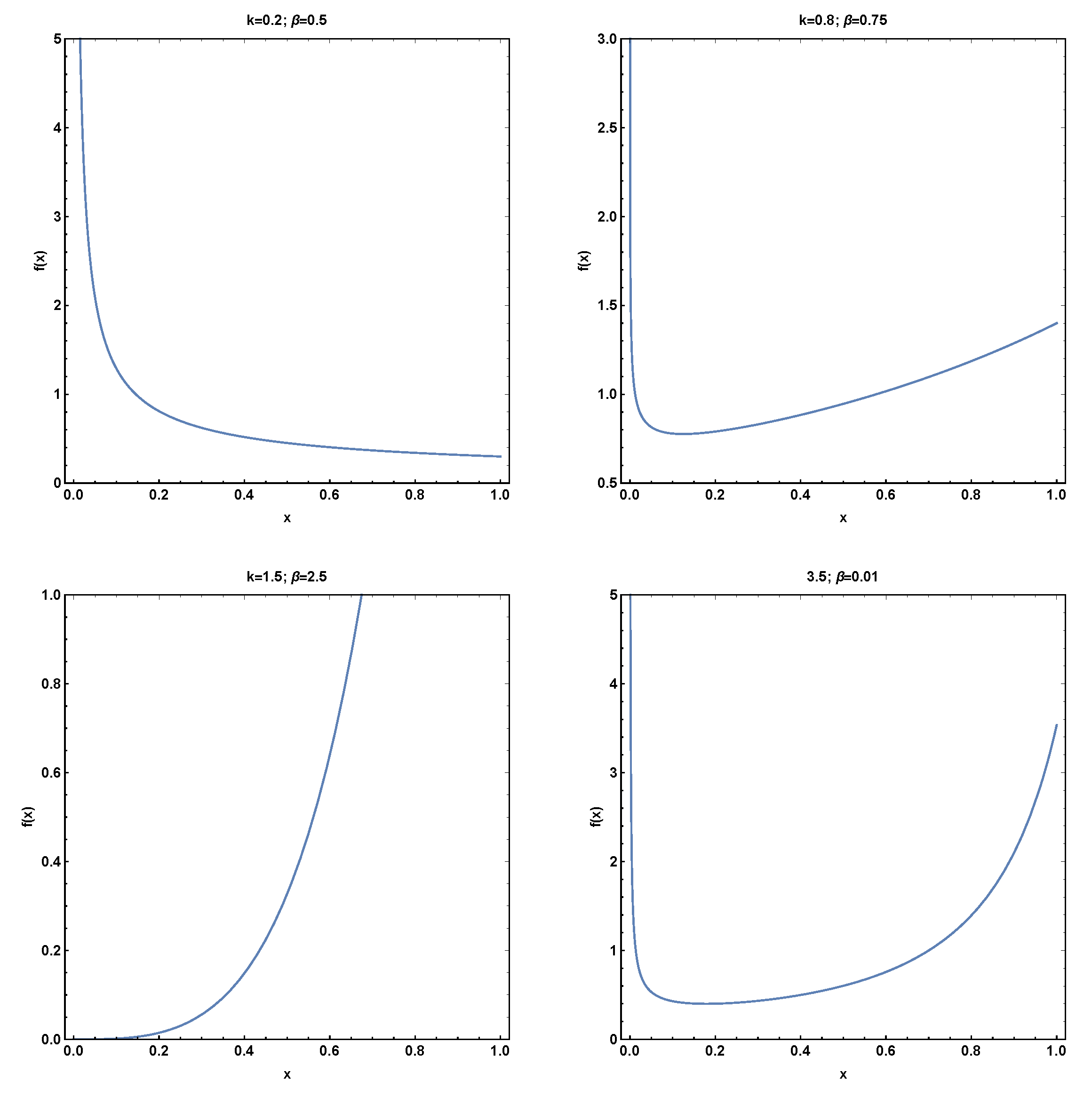
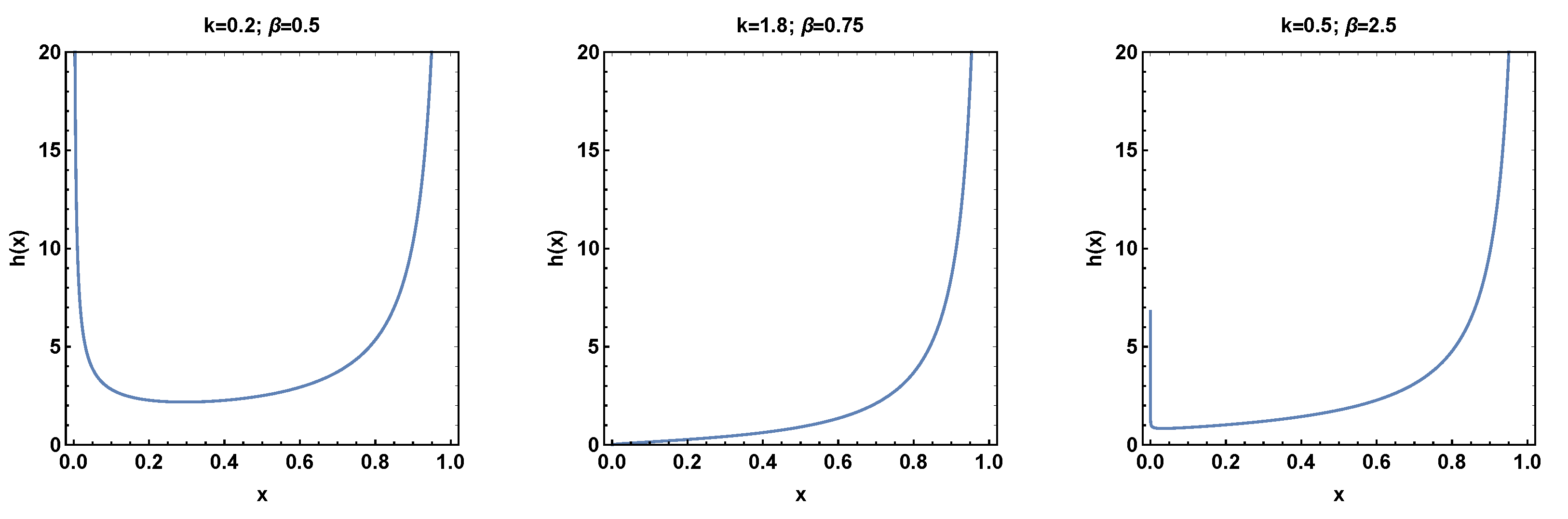
This research paper presents a significant contribution to the field of probability distributions by introducing a novel two-parameter bounded distribution using the power transformation method for generalization. The proposed distribution offers the capability to model a hazard rate function that exhibits both bathtub and increasing shapes. The bathtub-shaped hazard rate function is particularly interesting in various domains as it accurately captures the failure rates observed in certain real-world scenarios. To assess the effectiveness of the newly proposed model, an empirical investigation was conducted utilizing a real dataset from the COVID-19 pandemic. The model’s efficacy in practical applications could be evaluated by employing the proposed two-parameter distribution and comparing its performance with several existing distributions. The empirical analysis yielded valuable insights into the capabilities and advantages of the novel two-parameter distribution when applied to real-world data. This study significantly contributes to the existing body of knowledge by demonstrating the applicability and usefulness of the new distribution in capturing the complexities present in real datasets. By incorporating the proposed model, researchers and practitioners gain a powerful tool to accurately model and analyze datasets with bathtub-shaped hazard rate functions. Such modeling capabilities enhance understanding of failure rates and enable more precise decision making in various domains, including public health, engineering, and finance.

The paper is structured as follows. Section 2 defines the proposed distribution, including its PDF and CDF. In Section 3, we present the mathematical derivation of the associated properties and equations of the proposed model. Section 4 explains the methods and techniques used for the estimation process. To compare the performance of these estimation methods, a simulation study is conducted in Section 5. In Section 6, we analyze the efficiency of the proposed distribution by applying it to a real dataset of COVID-19 cases from various life applications and compare it to other distributions. Finally, in Section 7, we present the conclusions and major findings of the study.

2. Model Formulation

In (2022), Sağlam and Karakaya [12] presented a unit distribution called unit Burr–Hatke distribution (UBHD) with cumulative distribution function (CDF), defined as follows:

$$\begin{array}{cc}\hfill G\left(t\right)& =\frac{t^{\beta }}{1-log\left(t\right)},0<t<1,\beta >0,\hfill \end{array}$$

(1)

its probability density function (PDF) is defined as follows:

$$\begin{array}{cc}\hfill g\left(t\right)& =\frac{t^{\beta -1}(\beta +\beta (-log\left(t\right))+1)}{{(log\left(t\right)-1)}^2}.\hfill \end{array}$$

(2)

The power transformation $X=T^{\frac{1}{k}}$ is applied to the CDF (1) to have power unit Burr–Hatke distribution (PUBHD) with CDF defined as follows:

$$\begin{array}{c}\hfill F\left(x\right)=\frac{x^{\beta k}}{1-log\left(x^k\right)},0<x<1,k,\beta >0,\end{array}$$

(3)

we have PUBHD PDF defined as follows:

$$\begin{array}{c}\hfill f\left(x\right)=\frac{k{x}^{\beta k-1}\left(\beta +\beta \left(-log\left(x^k\right)\right)+1\right)}{{\left(log\left(x^k\right)-1\right)}^2}.\end{array}$$

(4)

The hazard function (HF) of PUBHD is defined as follows:

$$h\left(x\right)=\frac{k{x}^{\beta k-1}(\beta +\beta (-k)log\left(x\right)+1)}{(klog\left(x\right)-1)\left(x^{\beta k}+klog\left(x\right)-1\right)}.$$

(5)

Possible shapes for both PDF (4) and HF (5) are, respectively, presented in Figure 1 and Figure 2.

3. Statistical Properties

3.1. Quantile Function

The quantile function, also known as the inverse cumulative distribution function, is a fundamental concept in statistics and probability theory. It plays a crucial role in analyzing and interpreting data, especially when dealing with non-standard distributions or when determining specific points in a distribution. A quantile function is a powerful tool for understanding and utilizing the information contained within a probability distribution, making it an indispensable component in statistical analysis and decision making processes.

By obtaining the CDF (3) of the PUBHD, the quantile function (QF) of the PUBHD is obtained by calculating the inverse function of the CDF (3) as follows:

$$Q\left(u\right)={\left(\frac{uW\left(\frac{e^{\beta }\beta }{u}\right)}{\beta }\right)}^{\frac{1}{\beta k}},0<u<1,$$

(6)

where $W(·)$ is the Lambert function.

If u follows a uniform distribution, then the QF (6) is used to generate datasets of size n from the PUBHD by the following formula:

$$x_i={\left(\frac{u_{i}W\left(\frac{e^{\beta }\beta }{u_i}\right)}{\beta }\right)}^{\frac{1}{\beta k}},i=1,2,\dots ,n.$$

(7)

3.2. Moments

Moments about the origin play a crucial role in analyzing the distribution of a new system or quantity. When considering moments about the origin of a new distribution, engineers and researchers can gain valuable insights into the overall behavior and characteristics of the system. By calculating these moments, they can determine the distribution’s average position, spread, and symmetry. This information is vital for understanding the system’s properties, making predictions, and optimizing its design or performance. Moments about the origin allow for the quantification of important parameters, such as the center of mass, the variance, and even higher-order moments, which provide a deeper understanding and help capture the intricacies of the distribution. Whether in physics, statistics, or other scientific fields, moments about the origin serve as essential tools for analyzing and interpreting the behavior and properties of new distributions, allowing for more informed decision making and advancing knowledge in various domains.

The PUBHD’s hth moment is calculated as follows:

$$\begin{array}{c}\hfill {\mu }_r^{\prime }={\int }_0^{\infty }{x}^{r}f\left(x\right)dx=\frac{h{e}^{\beta +\frac{h}{k}}\mathrm{Ei}\left(-\frac{h+k\beta }{k}\right)}{k}+1,\end{array}$$

(8)

where $\mathrm{Ei}\left(z\right)=-{\int }_{-z}^{\infty }\frac{e^{-t}}{t}dt$. Measures such as the mean, variance, skewness, and kurtosis are commonly calculated alongside moments about the origin.

Table 1. Some numerical values for the PUBHD moments with CV, skewness, and kurtosis.

Parameters		Measures
$\mathit{\beta }$	k	${\mathit{\mu }}_{\mathbf{1}}^{\prime }$	${\mathit{\mu }}_{\mathbf{2}}^{\prime }$	${\mathit{\mu }}_{\mathbf{3}}^{\prime }$	${\mathit{\mu }}_{\mathbf{4}}^{\prime }$	${\mathit{\sigma }}^{\mathbf{2}}$	CV	Skewness	Kurtosis
0.1	0.1	0.09273	0.05017	0.03443	0.02621	0.04157	2.19887	2.60337	24.05780
	0.5	0.30401	0.19171	0.14105	0.11182	0.09929	1.03649	0.71578	32.01571
	1.0	0.44125	0.30401	0.23454	0.19171	0.10930	0.74926	0.10893	58.28333
	1.5	0.52637	0.38222	0.30401	0.25368	0.10515	0.61605	−0.23095	95.05568
	2.0	0.58603	0.44125	0.35877	0.30401	0.09782	0.53368	−0.47295	143.01398
	3.5	0.69455	0.55853	0.47353	0.41359	0.07614	0.39727	−0.95956	366.37956
0.7	0.1	0.13983	0.07653	0.05274	0.04024	0.05698	1.70716	1.91894	23.43719
	0.5	0.42916	0.28084	0.20979	0.16773	0.09666	0.72444	0.20963	67.69790
	1.0	0.59134	0.42916	0.33895	0.28084	0.07947	0.47672	−0.39358	216.71068
	1.5	0.68030	0.52431	0.42916	0.36431	0.06150	0.36452	−0.73477	523.34808
	2.0	0.73703	0.59134	0.49652	0.42916	0.04813	0.29765	−0.97163	1064.5
	3.5	0.82795	0.71147	0.62617	0.56047	0.02597	0.19465	−1.41023	5085.71
1.0	0.1	0.16158	0.08917	0.06163	0.04710	0.06306	1.55416	1.69514	24.0789
	0.5	0.47583	0.31831	0.24015	0.19310	0.09189	0.63708	0.04443	94.5673
	1.0	0.63867	0.47583	0.38096	0.31831	0.06793	0.40809	−0.54838	361.374
	1.5	0.72351	0.57261	0.47583	0.40793	0.04915	0.30641	−0.87887	968.205
	2.0	0.77587	0.63867	0.54471	0.47583	0.03669	0.24689	−1.10345	2113.36
	3.5	0.85688	0.75245	0.67227	0.60847	0.01821	0.15750	−1.50364	11,425.7
2.0	0.1	0.22674	0.12891	0.09012	0.06929	0.07750	1.22779	1.19328	28.446
	0.5	0.58731	0.41893	0.32632	0.26749	0.07400	0.46317	−0.32977	243.63
	1.0	0.73792	0.58731	0.48873	0.41893	0.04279	0.28032	−0.88121	1347.01
	1.5	0.80781	0.67953	0.58731	0.51761	0.02697	0.20328	−1.17117	4388.41
	2.0	0.84824	0.73792	0.65377	0.58731	0.01841	0.15996	−1.35679	10,850.9
	3.5	0.90692	0.83040	0.76627	0.71166	0.00790	0.09798	−1.66010	71,863.04
2.5	0.1	0.25565	0.14751	0.10372	0.07999	0.08215	1.12115	1.01971	31.562
	0.5	0.62672	0.45876	0.36242	0.29975	0.06599	0.40988	−0.46022	362.6493
	1.0	0.76918	0.62672	0.52951	0.45876	0.03508	0.24349	−0.99079	2252.86
	1.5	0.83284	0.71481	0.62672	0.55831	0.02118	0.17476	−1.26220	7767.72
	2.0	0.86896	0.76918	0.69048	0.62672	0.01409	0.13661	−1.43206	19,876.9
	3.5	0.92048	0.85309	0.79519	0.74487	0.00581	0.08280	−1.70189	13,8750.7
3.0	0.1	0.28246	0.16532	0.11692	0.09046	0.08554	1.03540	0.87562	35.213
	0.5	0.65916	0.49344	0.39483	0.32927	0.05895	0.36834	−0.56847	519.733
	1.0	0.79365	0.65916	0.56420	0.49344	0.02927	0.21556	−1.07897	3538.76
	1.5	0.85198	0.74297	0.65916	0.59260	0.01710	0.15349	−1.33363	12,738.8
	2.0	0.88459	0.79365	0.72004	0.65916	0.01115	0.11939	−1.49001	33,441.04
	3.5	0.93051	0.87031	0.81762	0.77109	0.00447	0.07181	−1.73298	242,550.3

presents numerical values for moments about the origin, as well as related measures, including the coefficient of variation, coefficient of skewness, and coefficient of kurtosis, for various values of parameters $\beta$ and k. These values correspond to the PUBHD distribution. The relationship between the parameter values (specifically $\beta$ and k) and the measure values in Table 1 can provide insights into how these parameters impact the statistical properties of the PUBHD distribution. Here are some observations:

• As the parameter $\beta$ increases, both the mean and variance tend to increase. This indicates that a higher value of $\beta$ leads to a shift in the distribution towards larger values, resulting in a greater spread or dispersion.
• The coefficient of variation generally decreases as $\beta$ increases. This suggests that, as the distribution becomes more concentrated around its mean, the relative variability decreases.
• The skewness coefficient, which measures the asymmetry of the distribution, varies depending on the parameter values. For a fixed value of $\beta$, as k increases, the skewness tends to decrease, indicating a more symmetric distribution. However, as $\beta$ increases, the skewness can exhibit varying trends depending on the specific value of k.
• The kurtosis coefficient measures the peakedness or flatness of the distribution compared to a normal distribution. As $\beta$ increases, the kurtosis increases, indicating heavier tails and a more peaked distribution.

These observations demonstrate the parameter values’ influence on the PUBHD distribution’s statistical properties. Understanding these relationships can help researchers and practitioners analyze and interpret data generated from the PUBHD distribution, enabling them to make informed decisions and draw meaningful conclusions.

3.3. Moment-Generating Function

The moment-generating function (MGF) is closely related to moments about the origin. The moment-generating function of a random variable is a mathematical function that uniquely characterizes its probability distribution. It provides a systematic way to compute moments of the random variable by taking derivatives of the MGF at the origin. Specifically, the nth derivative of the MGF at zero corresponds to the nth moment about the origin. The MGF of PUBHD is determined as follows:

$$\begin{array}{c}\hfill MGF={\int }_0^{\infty }{e}^{hx}f\left(x\right)dx=\sum _{r=0}^{\infty }\frac{h^r}{r!}\left[\frac{h{e}^{\beta +\frac{h}{k}}\mathrm{Ei}\left(-\frac{h+k\beta }{k}\right)}{k}+1\right].\end{array}$$

(9)

3.4. Order Statistics

Order statistics refers to the branch of statistics that deals with studying and analyzing the characteristics of a set of ordered observations or data points. It focuses on understanding the properties and behavior of various statistical measures associated with data ordering, such as the minimum, maximum, median, quartiles, and percentiles. Order statistics play a crucial role in various fields, including economics, finance, biology, and engineering, as they provide valuable insights into the distribution and variability of data. By examining the order of observations, researchers can make informed decisions, draw meaningful conclusions, and make accurate predictions based on the underlying statistical properties of the dataset.

The $i\mathrm{th}$ order statistics for the PDF and CDF of PUBHD are derived, respectively, as follows:

$$\begin{array}{cc}\hfill f_{i:n}\left(x\right)& =\frac{n!}{(i-1)!(n-i)!}{\left[F\left(x\right)\right]}^{i-1}{[1-F\left(x\right)]}^{n-i}f\left(x\right)\hfill \\ \hfill & =\frac{n!x^{\beta k}{\left(\frac{k{x}^{\beta k-1}(\beta +\beta (-k)log\left(x\right)+1)}{{(klog\left(x\right)-1)}^2}\right)}^{i-1}{\left(\frac{k{x}^{\beta k-1}(-\beta +\beta klog\left(x\right)-1)}{{(klog\left(x\right)-1)}^2}+1\right)}^{n-i}}{\mathrm{\Gamma }\left(i\right)\mathrm{\Gamma }(-i+n+1)(1-klog(x\left)\right)},\hfill \\ \hfill F_{i:n}\left(x\right)& =\sum _{r=i}^n{(}_r^n){\left(F\left(x\right)\right)}^r{(1-F\left(x\right))}^{n-r}=\frac{\mathrm{\Gamma }(n+1)}{\mathrm{\Gamma }(-i+n+1)}{\left(\frac{k{x}^{\beta k-1}(\beta +\beta (-k)log\left(x\right)+1)}{{(klog\left(x\right)-1)}^2}\right)}^i\hfill \\ \hfill & {\left(\frac{k{x}^{\beta k-1}(-\beta +\beta klog\left(x\right)-1)}{{(klog\left(x\right)-1)}^2}+1\right)}^{n-i}{}_2{\tilde{F}}_1\left(1,i-n;i+1;\frac{1}{\frac{{(klog\left(x\right)-1)}^2{x}^{1-k\beta }}{k(klog(x)\beta -\beta -1)}+1}\right).\hfill \end{array}$$

4. Estimation Methods

In this section, we discuss the conventional parameter estimation methods for the PUBHD. These methods involve maximizing or minimizing an objective function to obtain the estimator. For more details, see [13,14,15].

The parameter estimation for PUBHD is obtained through maximum likelihood estimation ($Est{.}_1$) by maximizing the following equation.

$$\begin{array}{c}\hfill logL=\sum _{i=1}^{n}log\left(\beta +\beta \left(-log\left(x_i^k\right)\right)+1\right)+(\beta k-1)\sum _{i=1}^{n}log\left(x_i\right)-2\sum _{i=1}^{n}log\left(1-log\left(x_i^k\right)\right)+nlog\left(k\right).\end{array}$$

The parameter estimation for PUBHD is obtained through Anderson–Darling estimation ($Est{.}_2$) by minimizing the following equation.

$$\begin{array}{cc}\hfill A& =-n-\frac{1}{n}\sum _{i=1}^n(2i-1)[logF\left(x_i\right)+logS\left(x_i\right)]\hfill \\ \hfill & =-n-\frac{1}{n}\sum _{i=1}^n(2i-1)[log\left(\frac{x_i^{\beta k}}{1-log\left(x_i^k\right)}\right)+log\left(1-\frac{x_i^{\beta k}}{1-log\left(x_i^k\right)}\right)].\hfill \end{array}$$

The parameter estimation for PUBHD is obtained through Cramér–von Mises estimation ($Est{.}_3$) by minimizing the following equation.

$$\begin{array}{cc}\hfill C\left(x_i\right)& =-\frac{1}{12n}+\sum _{i=1}^n{\left[F\left(x_i\right)-\frac{2i-1}{2n}\right]}^2\hfill \\ \hfill & =-\frac{1}{12n}+\sum _{i=1}^n{\left[\left(\frac{x_i^{\beta k}}{1-log\left(x_i^k\right)}\right)-\frac{2i-1}{2n}\right]}^2\hfill \end{array}$$

The parameter estimation for PUBHD is obtained through maximum product of the spacings estimation ($Est{.}_4$) by maximizing the following equation.

$$T=\frac{1}{n+1}\sum _{i=1}^{n+1}log{E}_i,E_i=F\left(x_{\left(i\right)}\right)-F\left(x_{(i-1)}\right).$$

The parameter estimation for PUBHD is obtained through least-squares estimation ($Est{.}_5$) by minimizing the following equation.

$$\begin{array}{cc}\hfill LS& =\sum _{i=1}^n{\left[F\left(x_i\right)-\frac{i}{n+1}\right]}^2=\sum _{i=1}^n{\left[\left(\frac{x_i^{\beta k}}{1-log\left(x_i^k\right)}\right)-\frac{i}{n+1}\right]}^2.\hfill \end{array}$$

The parameter estimation for PUBHD is obtained through right-tail Anderson–Darling estimation ($Est{.}_6$) by minimizing the following equation.

$$\begin{array}{cc}\hfill R& =\frac{n}{2}-2\sum _{i=1}^{n}F\left(x_i\right)-\frac{1}{n}\sum _{i=1}^n\left(2i-1\right)logS\left(x_{n+1-i}\right)\hfill \\ \hfill & =\frac{n}{2}-2\sum _{i=1}^n\frac{x_i^{\beta k}}{1-log\left(x_i^k\right)}-\frac{1}{n}\sum _{i=1}^n\left(2i-1\right)log\frac{x_{n+1-i}^{\beta k}}{1-log\left(x_{n+1-i}^k\right)}.\hfill \end{array}$$

The parameter estimation for PUBHD is obtained through weighted least square estimation ($Est{.}_7$) by minimizing the following equation.

$$W=\sum _{i=1}^n\frac{{(n+1)}^2(n+2)}{i(n-i+1)}{\left[F\left(x_i\right)-\frac{i}{n+1}\right]}^2=\sum _{i=1}^n\frac{{(n+1)}^2(n+2)}{i(n-i+1)}{\left[\frac{x_i^{\beta k}}{1-log\left(x_i^k\right)}-\frac{i}{n+1}\right]}^2.$$

The parameter estimation for PUBHD is obtained through left-tailed Anderson–Darling estimation ($Est{.}_8$) by minimizing the following equation.

$$\begin{array}{cc}\hfill LT& =-\frac{3}{2}n+2\sum _{i=1}^{n}F\left(x_i\right)-\frac{1}{n}\sum _{i=1}^n(2i-1)logF\left(x_i\right)\hfill \\ \hfill & =-\frac{3}{2}n+2\sum _{i=1}^n\frac{x_i^{\beta k}}{1-log\left(x_i^k\right)}-\frac{1}{n}\sum _{i=1}^n(2i-1)log\frac{x_i^{\beta k}}{1-log\left(x_i^k\right)}.\hfill \end{array}$$

The parameter estimation for PUBHD is obtained through minimum spacing absolute distance estimation ($Est{.}_9$) by minimizing the following equation.

$$\begin{array}{cc}\hfill M{S}_1& =\sum _{i=1}^{n+1}|E_i-\frac{1}{n+1}|.\hfill \end{array}$$

The parameter estimation for PUBHD is obtained through minimum spacing absolute-log distance estimation ($Est{.}_{10}$) by minimizing the following equation.

$$\begin{array}{cc}\hfill M{S}_2& =\sum _{i=1}^{n+1}|log{E}_i-log\frac{1}{n+1}|.\hfill \end{array}$$

The parameter estimation for PUBHD is obtained through Anderson–Darling left-tail second-order estimation ($Est{.}_{11}$) by minimizing the following equation.

$$\begin{array}{cc}\hfill LTS& =2\sum _{i=1}^{n}logF\left(x_i\right)+\frac{1}{n}\sum _{i=1}^n\frac{(2i-1)}{F\left(x_i\right)}\hfill \\ \hfill & =2\sum _{i=1}^{n}log\frac{x_i^{\beta k}}{1-log\left(x_i^k\right)}+\frac{1}{n}\sum _{i=1}^n\frac{(2i-1)[1-log\left(x_i^k\right)]}{x_i^{\beta k}}.\hfill \end{array}$$

The parameter estimation for PUBHD is obtained through Kolmogorov estimation ($Est{.}_{12}$) by minimizing the following equation.

$$\begin{array}{c}\hfill KM=MA{X}_{1\le i\le n}\left[\frac{i}{n}-F\left(x_i\right),F\left(x_i\right)-\frac{i-1}{n}\right]\end{array}$$

5. Numerical Simulation

In this section, we will employ all the estimating methods discussed earlier to identify estimators for our proposed model using randomly generated datasets. The objective of this study is to investigate the behavior and performance of these estimating approaches. To evaluate the success of these methods, various measurements will be utilized, including the average of bias (BIAS), mean squared errors (MSE), and mean relative errors (MRE), which will be calculated for different parameter combinations and sample sizes using the R programming language. A simulation will be conducted to determine the most accurate approach for estimating the model parameters. In this simulation, we will generate 1000 samples with varying sizes (30, 60, 100, 150, 200, and 300). The numerical outcomes of the simulations are presented in

Table 2. Simulation values of BIAS, MSE, and MRE for $k=0.75,\beta =0.25$.

n	Est.	Est.Par.	$\mathit{Est}{.}_1$	$\mathit{Est}{.}_2$	$\mathit{Est}{.}_3$	$\mathit{Est}{.}_4$	$\mathit{Est}{.}_5$	$\mathit{Est}{.}_6$	$\mathit{Est}{.}_7$	$\mathit{Est}{.}_8$	$\mathit{Est}{.}_9$	$\mathit{Est}{.}_{10}$	$\mathit{Est}{.}_{11}$	$\mathit{Est}{.}_{12}$
30	BIAS	$\widehat{k}$	0.2242${}^{\left\{4\right\}}$	$0.{22761}^{\left\{6\right\}}$	$0.{22953}^{\left\{7\right\}}$	$0.{23828}^{\left\{10\right\}}$	$0.{23396}^{\left\{9\right\}}$	$0.{23898}^{\left\{11\right\}}$	$0.{23223}^{\left\{8\right\}}$	$0.{22349}^{\left\{3\right\}}$	$0.{19765}^{\left\{2\right\}}$	$0.{22559}^{\left\{5\right\}}$	$0.{24253}^{\left\{12\right\}}$	$0.{17698}^{\left\{1\right\}}$
		$\widehat{\beta }$	$0.{10723}^{\left\{2\right\}}$	$0.{12459}^{\left\{6\right\}}$	$0.{12883}^{\left\{10\right\}}$	$0.{1287}^{\left\{9\right\}}$	$0.{13719}^{\left\{12\right\}}$	$0.{13161}^{\left\{11\right\}}$	$0.{12793}^{\left\{8\right\}}$	$0.{11786}^{\left\{4\right\}}$	$0.{11714}^{\left\{3\right\}}$	$0.{12495}^{\left\{7\right\}}$	$0.{1207}^{\left\{5\right\}}$	$0.{10111}^{\left\{1\right\}}$
	MSE	$\widehat{k}$	$0.{08022}^{\left\{4\right\}}$	$0.{08198}^{\left\{5\right\}}$	$0.{08654}^{\left\{9\right\}}$	$0.{08932}^{\left\{11\right\}}$	$0.{08597}^{\left\{8\right\}}$	$0.{08915}^{\left\{10\right\}}$	$0.{08414}^{\left\{7\right\}}$	$0.{07979}^{\left\{3\right\}}$	$0.{07062}^{\left\{2\right\}}$	$0.{08331}^{\left\{6\right\}}$	$0.{09092}^{\left\{12\right\}}$	$0.{05269}^{\left\{1\right\}}$
		$\widehat{\beta }$	$0.{01559}^{\left\{2\right\}}$	$0.{02013}^{\left\{6\right\}}$	$0.{02154}^{\left\{10\right\}}$	$0.{0212}^{\left\{8\right\}}$	$0.{02404}^{\left\{12\right\}}$	$0.{02268}^{\left\{11\right\}}$	$0.{02131}^{\left\{9\right\}}$	$0.{01845}^{\left\{4\right\}}$	$0.{01834}^{\left\{3\right\}}$	$0.{02061}^{\left\{7\right\}}$	$0.{01863}^{\left\{5\right\}}$	$0.{01516}^{\left\{1\right\}}$
	MRE	$\widehat{k}$	$0.{29893}^{\left\{3\right\}}$	$0.{30348}^{\left\{5\right\}}$	$0.{30604}^{\left\{6\right\}}$	$0.{3177}^{\left\{9\right\}}$	$0.{31195}^{\left\{8\right\}}$	$0.{31864}^{\left\{10\right\}}$	$0.{30964}^{\left\{7\right\}}$	$0.{29799}^{\left\{2\right\}}$	$0.{26353}^{\left\{1\right\}}$	$0.{30078}^{\left\{4\right\}}$	$0.{32337}^{\left\{11.5\right\}}$	$0.{32337}^{\left\{11.5\right\}}$
		$\widehat{\beta }$	$0.{42891}^{\left\{2\right\}}$	$0.{49837}^{\left\{5\right\}}$	$0.{51532}^{\left\{9\right\}}$	$0.{51478}^{\left\{8\right\}}$	$0.{54875}^{\left\{11\right\}}$	$0.{52643}^{\left\{10\right\}}$	$0.{51172}^{\left\{7\right\}}$	$0.{47145}^{\left\{4\right\}}$	$0.{46857}^{\left\{3\right\}}$	$0.{49979}^{\left\{6\right\}}$	$0.{78642}^{\left\{12\right\}}$	$0.{23597}^{\left\{1\right\}}$
	$\sum Ranks$		${17}^{\left\{3\right\}}$	${33}^{\left\{5\right\}}$	${51}^{\left\{8\right\}}$	${55}^{\left\{9\right\}}$	${60}^{\left\{11\right\}}$	${63}^{\left\{12\right\}}$	${46}^{\left\{7\right\}}$	${20}^{\left\{4\right\}}$	${14}^{\left\{1\right\}}$	${35}^{\left\{6\right\}}$	$57.5^{\left\{10\right\}}$	$16.5^{\left\{2\right\}}$
60	BIAS	$\widehat{k}$	$0.{17144}^{\left\{3\right\}}$	$0.{19554}^{\left\{5\right\}}$	$0.{20388}^{\left\{9\right\}}$	$0.{2015}^{\left\{7\right\}}$	$0.{21103}^{\left\{10\right\}}$	$0.{2111}^{\left\{11\right\}}$	$0.{20235}^{\left\{8\right\}}$	$0.{18606}^{\left\{4\right\}}$	$0.{1668}^{\left\{2\right\}}$	$0.{21213}^{\left\{12\right\}}$	$0.{19926}^{\left\{6\right\}}$	$0.{15566}^{\left\{1\right\}}$
		$\widehat{\beta }$	$0.{09798}^{\left\{2\right\}}$	$0.{10985}^{\left\{6\right\}}$	$0.{11491}^{\left\{9\right\}}$	$0.{11283}^{\left\{8\right\}}$	$0.{12336}^{\left\{11\right\}}$	$0.{12886}^{\left\{12\right\}}$	$0.{11038}^{\left\{7\right\}}$	$0.{10488}^{\left\{4\right\}}$	$0.{0984}^{\left\{3\right\}}$	$0.{11573}^{\left\{10\right\}}$	$0.{10779}^{\left\{5\right\}}$	$0.{09717}^{\left\{1\right\}}$
	MSE	$\widehat{k}$	$0.{04781}^{\left\{2\right\}}$	$0.{06325}^{\left\{5\right\}}$	$0.{06926}^{\left\{9\right\}}$	$0.{06579}^{\left\{7\right\}}$	$0.{07345}^{\left\{11\right\}}$	$0.{07298}^{\left\{10\right\}}$	$0.{06835}^{\left\{8\right\}}$	$0.{05605}^{\left\{4\right\}}$	$0.{05353}^{\left\{3\right\}}$	$0.{07582}^{\left\{12\right\}}$	$0.{06541}^{\left\{6\right\}}$	$0.{04213}^{\left\{1\right\}}$
		$\widehat{\beta }$	$0.{01353}^{\left\{1\right\}}$	$0.{01616}^{\left\{6\right\}}$	$0.{01796}^{\left\{10\right\}}$	$0.{01658}^{\left\{8\right\}}$	$0.{02008}^{\left\{11\right\}}$	$0.{02153}^{\left\{12\right\}}$	$0.{01647}^{\left\{7\right\}}$	$0.{0149}^{\left\{4\right\}}$	$0.{01365}^{\left\{2\right\}}$	$0.{01762}^{\left\{9\right\}}$	$0.{01546}^{\left\{5\right\}}$	$0.{01383}^{\left\{3\right\}}$
	MRE	$\widehat{k}$	$0.{22859}^{\left\{2\right\}}$	$0.{26072}^{\left\{4\right\}}$	$0.{27184}^{\left\{9\right\}}$	$0.{26866}^{\left\{7\right\}}$	$0.{28138}^{\left\{10\right\}}$	$0.{28147}^{\left\{11\right\}}$	$0.{26981}^{\left\{8\right\}}$	$0.{24808}^{\left\{3\right\}}$	$0.{22241}^{\left\{1\right\}}$	$0.{28285}^{\left\{12\right\}}$	$0.{26569}^{\left\{5.5\right\}}$	$0.{26569}^{\left\{5.5\right\}}$
		$\widehat{\beta }$	$0.{3919}^{\left\{2\right\}}$	$0.{43941}^{\left\{5\right\}}$	$0.{45965}^{\left\{8\right\}}$	$0.{45134}^{\left\{7\right\}}$	$0.{49343}^{\left\{10\right\}}$	$0.{51542}^{\left\{11\right\}}$	$0.{44152}^{\left\{6\right\}}$	$0.{41954}^{\left\{4\right\}}$	$0.{39361}^{\left\{3\right\}}$	$0.{4629}^{\left\{9\right\}}$	$0.{79382}^{\left\{12\right\}}$	$0.{20755}^{\left\{1\right\}}$
	$\sum Ranks$		${12}^{\left\{1\right\}}$	${31}^{\left\{5\right\}}$	${54}^{\left\{9\right\}}$	${44}^{\left\{7.5\right\}}$	${63}^{\left\{10\right\}}$	${67}^{\left\{12\right\}}$	${44}^{\left\{7.5\right\}}$	${23}^{\left\{4\right\}}$	${14}^{\left\{3\right\}}$	${64}^{\left\{11\right\}}$	$39.5^{\left\{6\right\}}$	$12.5^{\left\{2\right\}}$
100	BIAS	$\widehat{k}$	$0.{14271}^{\left\{2\right\}}$	$0.{15641}^{\left\{4\right\}}$	$0.{17132}^{\left\{10\right\}}$	$0.{16442}^{\left\{7\right\}}$	$0.{16918}^{\left\{9\right\}}$	$0.{20087}^{\left\{12\right\}}$	$0.{15946}^{\left\{6\right\}}$	$0.{14484}^{\left\{3\right\}}$	$0.{15765}^{\left\{5\right\}}$	$0.{16512}^{\left\{8\right\}}$	$0.{17619}^{\left\{11\right\}}$	$0.{13774}^{\left\{1\right\}}$
		$\widehat{\beta }$	$0.{08956}^{\left\{1\right\}}$	$0.{10077}^{\left\{9\right\}}$	$0.{1092}^{\left\{11\right\}}$	$0.{09385}^{\left\{5\right\}}$	$0.{10846}^{\left\{10\right\}}$	$0.{12498}^{\left\{12\right\}}$	$0.{0995}^{\left\{7\right\}}$	$0.{09223}^{\left\{4\right\}}$	$0.{09054}^{\left\{2\right\}}$	$0.{10007}^{\left\{8\right\}}$	$0.{09795}^{\left\{6\right\}}$	$0.{09204}^{\left\{3\right\}}$
	MSE	$\widehat{k}$	$0.{03262}^{\left\{1\right\}}$	$0.{04081}^{\left\{4\right\}}$	$0.{04866}^{\left\{9\right\}}$	$0.{04319}^{\left\{6\right\}}$	$0.{0488}^{\left\{10\right\}}$	$0.{0656}^{\left\{12\right\}}$	$0.{04256}^{\left\{5\right\}}$	$0.{03627}^{\left\{3\right\}}$	$0.{04581}^{\left\{7\right\}}$	$0.{04585}^{\left\{8\right\}}$	$0.{05068}^{\left\{11\right\}}$	$0.{03301}^{\left\{2\right\}}$
		$\widehat{\beta }$	$0.{01156}^{\left\{1\right\}}$	$0.{0139}^{\left\{9\right\}}$	$0.{01617}^{\left\{11\right\}}$	$0.{01219}^{\left\{4\right\}}$	$0.{01605}^{\left\{10\right\}}$	$0.{02051}^{\left\{12\right\}}$	$0.{01361}^{\left\{7\right\}}$	$0.{01188}^{\left\{2\right\}}$	$0.{012}^{\left\{3\right\}}$	$0.{0137}^{\left\{8\right\}}$	$0.{01297}^{\left\{6\right\}}$	$0.{01247}^{\left\{5\right\}}$
	MRE	$\widehat{k}$	$0.{19029}^{\left\{1\right\}}$	$0.{20855}^{\left\{3\right\}}$	$0.{22842}^{\left\{9\right\}}$	$0.{21922}^{\left\{6\right\}}$	$0.{22557}^{\left\{8\right\}}$	$0.{26783}^{\left\{12\right\}}$	$0.{21261}^{\left\{5\right\}}$	$0.{19312}^{\left\{2\right\}}$	$0.{2102}^{\left\{4\right\}}$	$0.{22017}^{\left\{7\right\}}$	$0.{23492}^{\left\{10.5\right\}}$	$0.{23492}^{\left\{10.5\right\}}$
		$\widehat{\beta }$	$0.{35823}^{\left\{2\right\}}$	$0.{40307}^{\left\{8\right\}}$	$0.{43679}^{\left\{10\right\}}$	$0.{37538}^{\left\{5\right\}}$	$0.{43386}^{\left\{9\right\}}$	$0.{4999}^{\left\{11\right\}}$	$0.{39798}^{\left\{6\right\}}$	$0.{36891}^{\left\{4\right\}}$	$0.{36216}^{\left\{3\right\}}$	$0.{40027}^{\left\{7\right\}}$	$0.{7935}^{\left\{12\right\}}$	$0.{18366}^{\left\{1\right\}}$
	$\sum Ranks$		$8^{\left\{1\right\}}$	${37}^{\left\{7\right\}}$	${60}^{\left\{11\right\}}$	${33}^{\left\{5\right\}}$	${56}^{\left\{9\right\}}$	${71}^{\left\{12\right\}}$	${36}^{\left\{6\right\}}$	${18}^{\left\{2\right\}}$	${24}^{\left\{4\right\}}$	${46}^{\left\{8\right\}}$	$56.5^{\left\{10\right\}}$	$22.5^{\left\{3\right\}}$
150	BIAS	$\widehat{k}$	$0.{12205}^{\left\{2\right\}}$	$0.{13157}^{\left\{4\right\}}$	$0.{13976}^{\left\{8\right\}}$	$0.{13281}^{\left\{5\right\}}$	$0.{14656}^{\left\{9\right\}}$	$0.{16071}^{\left\{12\right\}}$	$0.{13437}^{\left\{6\right\}}$	$0.{12918}^{\left\{3\right\}}$	$0.{13701}^{\left\{7\right\}}$	$0.{15321}^{\left\{11\right\}}$	$0.{14909}^{\left\{10\right\}}$	$0.{11984}^{\left\{1\right\}}$
		$\widehat{\beta }$	$0.{08172}^{\left\{1\right\}}$	$0.{09073}^{\left\{8\right\}}$	$0.{09762}^{\left\{10\right\}}$	$0.{08629}^{\left\{4\right\}}$	$0.{09781}^{\left\{11\right\}}$	$0.{10776}^{\left\{12\right\}}$	$0.{08713}^{\left\{6\right\}}$	$0.{08652}^{\left\{5\right\}}$	$0.{08614}^{\left\{3\right\}}$	$0.{09168}^{\left\{9\right\}}$	$0.{08794}^{\left\{7\right\}}$	$0.{08238}^{\left\{2\right\}}$
	MSE	$\widehat{k}$	$0.{02414}^{\left\{1\right\}}$	$0.{02773}^{\left\{4\right\}}$	$0.{03201}^{\left\{7\right\}}$	$0.{02797}^{\left\{5\right\}}$	$0.{03686}^{\left\{10\right\}}$	$0.{04422}^{\left\{12\right\}}$	$0.{03042}^{\left\{6\right\}}$	$0.{02605}^{\left\{3\right\}}$	$0.{03401}^{\left\{8\right\}}$	$0.{03949}^{\left\{11\right\}}$	$0.{03641}^{\left\{9\right\}}$	$0.{02553}^{\left\{2\right\}}$
		$\widehat{\beta }$	$0.{00994}^{\left\{1\right\}}$	$0.{01181}^{\left\{8\right\}}$	$0.{01341}^{\left\{11\right\}}$	$0.{01023}^{\left\{2\right\}}$	$0.{01339}^{\left\{10\right\}}$	$0.{01614}^{\left\{12\right\}}$	$0.{01099}^{\left\{7\right\}}$	$0.{01085}^{\left\{5\right\}}$	$0.{01082}^{\left\{4\right\}}$	$0.{01188}^{\left\{9\right\}}$	$0.{01091}^{\left\{6\right\}}$	$0.{01038}^{\left\{3\right\}}$
	MRE	$\widehat{k}$	$0.{16274}^{\left\{1\right\}}$	$0.{17542}^{\left\{3\right\}}$	$0.{18635}^{\left\{7\right\}}$	$0.{17707}^{\left\{4\right\}}$	$0.{19542}^{\left\{8\right\}}$	$0.{21428}^{\left\{12\right\}}$	$0.{17916}^{\left\{5\right\}}$	$0.{17224}^{\left\{2\right\}}$	$0.{18269}^{\left\{6\right\}}$	$0.{20427}^{\left\{11\right\}}$	$0.{19878}^{\left\{9.5\right\}}$	$0.{19878}^{\left\{9.5\right\}}$
		$\widehat{\beta }$	$0.{32689}^{\left\{2\right\}}$	$0.{3629}^{\left\{7\right\}}$	$0.{39047}^{\left\{9\right\}}$	$0.{34515}^{\left\{4\right\}}$	$0.{39124}^{\left\{10\right\}}$	$0.{43105}^{\left\{11\right\}}$	$0.{34851}^{\left\{6\right\}}$	$0.{34609}^{\left\{5\right\}}$	$0.{34457}^{\left\{3\right\}}$	$0.{3667}^{\left\{8\right\}}$	$0.{77965}^{\left\{12\right\}}$	$0.{15979}^{\left\{1\right\}}$
	$\sum Ranks$		$8^{\left\{1\right\}}$	${34}^{\left\{6\right\}}$	${52}^{\left\{8\right\}}$	${24}^{\left\{4\right\}}$	${58}^{\left\{10\right\}}$	${71}^{\left\{12\right\}}$	${36}^{\left\{7\right\}}$	${23}^{\left\{3\right\}}$	${31}^{\left\{5\right\}}$	${59}^{\left\{11\right\}}$	$53.5^{\left\{9\right\}}$	$18.5^{\left\{2\right\}}$
200	BIAS	$\widehat{k}$	$0.{11137}^{\left\{2\right\}}$	$0.{12034}^{\left\{5\right\}}$	$0.{12651}^{\left\{8\right\}}$	$0.{12062}^{\left\{6\right\}}$	$0.{12688}^{\left\{9\right\}}$	$0.{13912}^{\left\{11\right\}}$	$0.{11994}^{\left\{4\right\}}$	$0.{11343}^{\left\{3\right\}}$	$0.{12445}^{\left\{7\right\}}$	$0.{13507}^{\left\{10\right\}}$	$0.{14397}^{\left\{12\right\}}$	$0.{10625}^{\left\{1\right\}}$
		$\widehat{\beta }$	$0.{07675}^{\left\{2\right\}}$	$0.{0831}^{\left\{7\right\}}$	$0.{0928}^{\left\{11\right\}}$	$0.{08046}^{\left\{3\right\}}$	$0.{09046}^{\left\{10\right\}}$	$0.{10021}^{\left\{12\right\}}$	$0.{08389}^{\left\{8\right\}}$	$0.{08047}^{\left\{4\right\}}$	$0.{08079}^{\left\{5\right\}}$	$0.{08269}^{\left\{6\right\}}$	$0.{08579}^{\left\{9\right\}}$	$0.{0767}^{\left\{1\right\}}$
	MSE	$\widehat{k}$	$0.{01889}^{\left\{1\right\}}$	$0.{02334}^{\left\{5\right\}}$	$0.{02481}^{\left\{7\right\}}$	$0.{02362}^{\left\{6\right\}}$	$0.{02646}^{\left\{8\right\}}$	$0.{03186}^{\left\{11\right\}}$	$0.{02212}^{\left\{4\right\}}$	$0.{01995}^{\left\{3\right\}}$	$0.{02868}^{\left\{9\right\}}$	$0.{02992}^{\left\{10\right\}}$	$0.{03424}^{\left\{12\right\}}$	$0.{01991}^{\left\{2\right\}}$
		$\widehat{\beta }$	$0.{00893}^{\left\{1\right\}}$	$0.{01013}^{\left\{7\right\}}$	$0.{01222}^{\left\{11\right\}}$	$0.{00922}^{\left\{2.5\right\}}$	$0.{01181}^{\left\{10\right\}}$	$0.{01414}^{\left\{12\right\}}$	$0.{01024}^{\left\{8\right\}}$	$0.{01009}^{\left\{6\right\}}$	$0.{00973}^{\left\{4\right\}}$	$0.{00993}^{\left\{5\right\}}$	$0.{01056}^{\left\{9\right\}}$	$0.{00922}^{\left\{2.5\right\}}$
	MRE	$\widehat{k}$	$0.{14849}^{\left\{1\right\}}$	$0.{16046}^{\left\{4\right\}}$	$0.{16868}^{\left\{7\right\}}$	$0.{16083}^{\left\{5\right\}}$	$0.{16917}^{\left\{8\right\}}$	$0.{18549}^{\left\{10\right\}}$	$0.{15992}^{\left\{3\right\}}$	$0.{15124}^{\left\{2\right\}}$	$0.{16593}^{\left\{6\right\}}$	$0.{1801}^{\left\{9\right\}}$	$0.{19195}^{\left\{11.5\right\}}$	$0.{19195}^{\left\{11.5\right\}}$
		$\widehat{\beta }$	$0.{30699}^{\left\{2\right\}}$	$0.{33242}^{\left\{7\right\}}$	$0.{37122}^{\left\{10\right\}}$	$0.{32184}^{\left\{3\right\}}$	$0.{36184}^{\left\{9\right\}}$	$0.{40083}^{\left\{11\right\}}$	$0.{33555}^{\left\{8\right\}}$	$0.{32187}^{\left\{4\right\}}$	$0.{32318}^{\left\{5\right\}}$	$0.{33077}^{\left\{6\right\}}$	$0.{77316}^{\left\{12\right\}}$	$0.{14167}^{\left\{1\right\}}$
	$\sum Ranks$		$9^{\left\{1\right\}}$	${35}^{\left\{5.5\right\}}$	${54}^{\left\{9.5\right\}}$	$25.5^{\left\{4\right\}}$	${54}^{\left\{9.5\right\}}$	${67}^{\left\{12\right\}}$	${35}^{\left\{5.5\right\}}$	${22}^{\left\{3\right\}}$	${36}^{\left\{7\right\}}$	${46}^{\left\{8\right\}}$	$65.5^{\left\{11\right\}}$	${19}^{\left\{2\right\}}$
300	BIAS	$\widehat{k}$	$0.{09372}^{\left\{2\right\}}$	$0.{09842}^{\left\{4\right\}}$	$0.{10848}^{\left\{8\right\}}$	$0.{103}^{\left\{6\right\}}$	$0.{1115}^{\left\{9\right\}}$	$0.{11659}^{\left\{11\right\}}$	$0.{09704}^{\left\{3\right\}}$	$0.{09845}^{\left\{5\right\}}$	$0.{10501}^{\left\{7\right\}}$	$0.{11268}^{\left\{10\right\}}$	$0.{12167}^{\left\{12\right\}}$	$0.{09193}^{\left\{1\right\}}$
		$\widehat{\beta }$	$0.{06666}^{\left\{1\right\}}$	$0.{07206}^{\left\{5\right\}}$	$0.{08394}^{\left\{10\right\}}$	$0.{06947}^{\left\{3\right\}}$	$0.{08836}^{\left\{11\right\}}$	$0.{09234}^{\left\{12\right\}}$	$0.{07324}^{\left\{7\right\}}$	$0.{07015}^{\left\{4\right\}}$	$0.{07269}^{\left\{6\right\}}$	$0.{07552}^{\left\{9\right\}}$	$0.{07547}^{\left\{8\right\}}$	$0.{06777}^{\left\{2\right\}}$
	MSE	$\widehat{k}$	$0.{01358}^{\left\{1\right\}}$	$0.{01593}^{\left\{5\right\}}$	$0.{018}^{\left\{7\right\}}$	$0.{01632}^{\left\{6\right\}}$	$0.{01907}^{\left\{8\right\}}$	$0.{0222}^{\left\{11\right\}}$	$0.{01443}^{\left\{2\right\}}$	$0.{01511}^{\left\{4\right\}}$	$0.{01956}^{\left\{9\right\}}$	$0.{02044}^{\left\{10\right\}}$	$0.{02335}^{\left\{12\right\}}$	$0.{01458}^{\left\{3\right\}}$
		$\widehat{\beta }$	$0.{00711}^{\left\{1\right\}}$	$0.{00822}^{\left\{6\right\}}$	$0.{0103}^{\left\{10\right\}}$	$0.{0072}^{\left\{2\right\}}$	$0.{01099}^{\left\{11\right\}}$	$0.{01198}^{\left\{12\right\}}$	$0.{00863}^{\left\{9\right\}}$	$0.{00757}^{\left\{4\right\}}$	$0.{00802}^{\left\{5\right\}}$	$0.{0086}^{\left\{8\right\}}$	$0.{0083}^{\left\{7\right\}}$	$0.{0074}^{\left\{3\right\}}$
	MRE	$\widehat{k}$	$0.{12496}^{\left\{1\right\}}$	$0.{13123}^{\left\{3\right\}}$	$0.{14464}^{\left\{7\right\}}$	$0.{13733}^{\left\{5\right\}}$	$0.{14867}^{\left\{8\right\}}$	$0.{15546}^{\left\{10\right\}}$	$0.{12939}^{\left\{2\right\}}$	$0.{13127}^{\left\{4\right\}}$	$0.{14002}^{\left\{6\right\}}$	$0.{15024}^{\left\{9\right\}}$	$0.{16223}^{\left\{11.5\right\}}$	$0.{16223}^{\left\{11.5\right\}}$
		$\widehat{\beta }$	$0.{26662}^{\left\{2\right\}}$	$0.{28823}^{\left\{5\right\}}$	$0.{33578}^{\left\{9\right\}}$	$0.{27787}^{\left\{3\right\}}$	$0.{35344}^{\left\{10\right\}}$	$0.{36937}^{\left\{11\right\}}$	$0.{29297}^{\left\{7\right\}}$	$0.{28059}^{\left\{4\right\}}$	$0.{29077}^{\left\{6\right\}}$	$0.{30208}^{\left\{8\right\}}$	$0.{76842}^{\left\{12\right\}}$	$0.{12257}^{\left\{1\right\}}$
	$\sum Ranks$		$8^{\left\{1\right\}}$	${28}^{\left\{5\right\}}$	${51}^{\left\{8\right\}}$	${25}^{\left\{3.5\right\}}$	${57}^{\left\{10\right\}}$	${67}^{\left\{12\right\}}$	${30}^{\left\{6\right\}}$	${25}^{\left\{3.5\right\}}$	${39}^{\left\{7\right\}}$	${54}^{\left\{9\right\}}$	$62.5^{\left\{11\right\}}$	$21.5^{\left\{2\right\}}$

,

Table 3. Simulation values of BIAS, MSE, and MRE for $k=2.0,\beta =1.5$.

n	Est.	Est.Par.	$\mathit{Est}{.}_1$	$\mathit{Est}{.}_2$	$\mathit{Est}{.}_3$	$\mathit{Est}{.}_4$	$\mathit{Est}{.}_5$	$\mathit{Est}{.}_6$	$\mathit{Est}{.}_7$	$\mathit{Est}{.}_8$	$\mathit{Est}{.}_9$	$\mathit{Est}{.}_{10}$	$\mathit{Est}{.}_{11}$	$\mathit{Est}{.}_{12}$
30	BIAS	$\widehat{k}$	0.79687${}^{\left\{2\right\}}$	$0.{84872}^{\left\{9\right\}}$	$0.{82126}^{\left\{5\right\}}$	$0.{85819}^{\left\{11\right\}}$	$0.{8413}^{\left\{8\right\}}$	$0.{85659}^{\left\{10\right\}}$	$0.{87871}^{\left\{12\right\}}$	$0.{82613}^{\left\{6\right\}}$	$0.{80223}^{\left\{3\right\}}$	$0.{83133}^{\left\{7\right\}}$	$0.{81713}^{\left\{4\right\}}$	$0.{78058}^{\left\{1\right\}}$
		$\widehat{\beta }$	$0.{60818}^{\left\{1\right\}}$	$0.{66193}^{\left\{6\right\}}$	$0.{64604}^{\left\{4\right\}}$	$0.{67108}^{\left\{8\right\}}$	$0.{68173}^{\left\{10\right\}}$	$0.{66819}^{\left\{7\right\}}$	$0.{6832}^{\left\{11\right\}}$	$0.{63224}^{\left\{2\right\}}$	$0.{66109}^{\left\{5\right\}}$	$0.{67638}^{\left\{9\right\}}$	$0.{6344}^{\left\{3\right\}}$	$0.{83152}^{\left\{12\right\}}$
	MSE	$\widehat{k}$	$0.{94105}^{\left\{2\right\}}$	$1.{04177}^{\left\{9\right\}}$	$0.{99298}^{\left\{6\right\}}$	$1.{0647}^{\left\{11\right\}}$	$1.{01867}^{\left\{8\right\}}$	$1.{05821}^{\left\{10\right\}}$	$1.{09347}^{\left\{12\right\}}$	$0.{98526}^{\left\{4\right\}}$	$0.{94547}^{\left\{3\right\}}$	$1.{00761}^{\left\{7\right\}}$	$0.{98935}^{\left\{5\right\}}$	$0.{81911}^{\left\{1\right\}}$
		$\widehat{\beta }$	$0.{48557}^{\left\{1\right\}}$	$0.{55095}^{\left\{5\right\}}$	$0.{54033}^{\left\{4\right\}}$	$0.{57147}^{\left\{8\right\}}$	$0.{58871}^{\left\{10\right\}}$	$0.{5714}^{\left\{7\right\}}$	$0.{58516}^{\left\{9\right\}}$	$0.{51554}^{\left\{2\right\}}$	$0.{56292}^{\left\{6\right\}}$	$0.{58964}^{\left\{11\right\}}$	$0.{5217}^{\left\{3\right\}}$	$0.{822}^{\left\{12\right\}}$
	MRE	$\widehat{k}$	$0.{39843}^{\left\{1\right\}}$	$0.{42436}^{\left\{9\right\}}$	$0.{41063}^{\left\{5\right\}}$	$0.{42909}^{\left\{11\right\}}$	$0.{42065}^{\left\{8\right\}}$	$0.{42694}^{\left\{10\right\}}$	$0.{43936}^{\left\{12\right\}}$	$0.{41307}^{\left\{6\right\}}$	$0.{40112}^{\left\{2\right\}}$	$0.{41567}^{\left\{7\right\}}$	$0.{40856}^{\left\{3.5\right\}}$	$0.{40856}^{\left\{3.5\right\}}$
		$\widehat{\beta }$	$0.{40546}^{\left\{2\right\}}$	$0.{44129}^{\left\{6\right\}}$	$0.{43069}^{\left\{4\right\}}$	$0.{44739}^{\left\{8\right\}}$	$0.{45448}^{\left\{10\right\}}$	$0.{44546}^{\left\{7\right\}}$	$0.{45547}^{\left\{11\right\}}$	$0.{42149}^{\left\{3\right\}}$	$0.{44073}^{\left\{5\right\}}$	$0.{45092}^{\left\{9\right\}}$	$1.{9332}^{\left\{12\right\}}$	$0.{39929}^{\left\{1\right\}}$
	$\sum Ranks$		$9^{\left\{1\right\}}$	${44}^{\left\{7\right\}}$	${28}^{\left\{4\right\}}$	${57}^{\left\{11\right\}}$	${54}^{\left\{10\right\}}$	${51}^{\left\{9\right\}}$	${67}^{\left\{12\right\}}$	${23}^{\left\{2\right\}}$	${24}^{\left\{3\right\}}$	${50}^{\left\{8\right\}}$	$30.5^{\left\{5.5\right\}}$	$30.5^{\left\{5.5\right\}}$
60	BIAS	$\widehat{k}$	$0.{7834}^{\left\{2\right\}}$	$0.{80926}^{\left\{5\right\}}$	$0.{81217}^{\left\{6\right\}}$	$0.{83188}^{\left\{11\right\}}$	$0.{82871}^{\left\{10\right\}}$	$0.{85468}^{\left\{12\right\}}$	$0.{81898}^{\left\{8\right\}}$	$0.{79205}^{\left\{3\right\}}$	$0.{79864}^{\left\{4\right\}}$	$0.{82083}^{\left\{9\right\}}$	$0.{81603}^{\left\{7\right\}}$	$0.{74978}^{\left\{1\right\}}$
		$\widehat{\beta }$	$0.{58591}^{\left\{1\right\}}$	$0.{62411}^{\left\{6\right\}}$	$0.{62303}^{\left\{5\right\}}$	$0.{62861}^{\left\{8\right\}}$	$0.{63736}^{\left\{9\right\}}$	$0.{64865}^{\left\{11\right\}}$	$0.{62726}^{\left\{7\right\}}$	$0.{61044}^{\left\{2\right\}}$	$0.{61878}^{\left\{4\right\}}$	$0.{64773}^{\left\{10\right\}}$	$0.{61566}^{\left\{3\right\}}$	$0.{78766}^{\left\{12\right\}}$
	MSE	$\widehat{k}$	$0.{91095}^{\left\{2\right\}}$	$0.{96954}^{\left\{5\right\}}$	$0.{98998}^{\left\{9\right\}}$	$1.{00791}^{\left\{11\right\}}$	$1.{00695}^{\left\{10\right\}}$	$1.{05225}^{\left\{12\right\}}$	$0.{98328}^{\left\{8\right\}}$	$0.{92366}^{\left\{3\right\}}$	$0.{94774}^{\left\{4\right\}}$	$0.{98013}^{\left\{7\right\}}$	$0.{97075}^{\left\{6\right\}}$	$0.{7817}^{\left\{1\right\}}$
		$\widehat{\beta }$	$0.{45481}^{\left\{1\right\}}$	$0.{50043}^{\left\{6\right\}}$	$0.{50737}^{\left\{7\right\}}$	$0.{49943}^{\left\{5\right\}}$	$0.{52019}^{\left\{9\right\}}$	$0.{53495}^{\left\{11\right\}}$	$0.{50923}^{\left\{8\right\}}$	$0.{48161}^{\left\{2\right\}}$	$0.{499}^{\left\{4\right\}}$	$0.{53242}^{\left\{10\right\}}$	$0.{4839}^{\left\{3\right\}}$	$0.{75809}^{\left\{12\right\}}$
	MRE	$\widehat{k}$	$0.{3917}^{\left\{1\right\}}$	$0.{40463}^{\left\{4\right\}}$	$0.{40609}^{\left\{5\right\}}$	$0.{41594}^{\left\{11\right\}}$	$0.{41435}^{\left\{10\right\}}$	$0.{42734}^{\left\{12\right\}}$	$0.{40949}^{\left\{8\right\}}$	$0.{39603}^{\left\{2\right\}}$	$0.{39932}^{\left\{3\right\}}$	$0.{41042}^{\left\{9\right\}}$	$0.{40802}^{\left\{6.5\right\}}$	$0.{40802}^{\left\{6.5\right\}}$
		$\widehat{\beta }$	$0.{39061}^{\left\{2\right\}}$	$0.{41607}^{\left\{6\right\}}$	$0.{41535}^{\left\{5\right\}}$	$0.{41907}^{\left\{8\right\}}$	$0.{42491}^{\left\{9\right\}}$	$0.{43243}^{\left\{11\right\}}$	$0.{41817}^{\left\{7\right\}}$	$0.{40696}^{\left\{3\right\}}$	$0.{41252}^{\left\{4\right\}}$	$0.{43182}^{\left\{10\right\}}$	$2.{07432}^{\left\{12\right\}}$	$0.{37489}^{\left\{1\right\}}$
	$\sum Ranks$		$9^{\left\{1\right\}}$	${32}^{\left\{4\right\}}$	${37}^{\left\{6\right\}}$	${54}^{\left\{9\right\}}$	${57}^{\left\{11\right\}}$	${69}^{\left\{12\right\}}$	${46}^{\left\{8\right\}}$	${15}^{\left\{2\right\}}$	${23}^{\left\{3\right\}}$	${55}^{\left\{10\right\}}$	$37.5^{\left\{7\right\}}$	$33.5^{\left\{5\right\}}$
100	BIAS	$\widehat{k}$	$0.{71926}^{\left\{1\right\}}$	$0.{76616}^{\left\{5\right\}}$	$0.{78812}^{\left\{6\right\}}$	$0.{8083}^{\left\{10\right\}}$	$0.{80157}^{\left\{8\right\}}$	$0.{8219}^{\left\{12\right\}}$	$0.{76608}^{\left\{4\right\}}$	$0.{75401}^{\left\{3\right\}}$	$0.{80692}^{\left\{9\right\}}$	$0.{80943}^{\left\{11\right\}}$	$0.{78994}^{\left\{7\right\}}$	$0.{74142}^{\left\{2\right\}}$
		$\widehat{\beta }$	$0.{57157}^{\left\{1\right\}}$	$0.{58919}^{\left\{2\right\}}$	$0.{60946}^{\left\{6\right\}}$	$0.{61007}^{\left\{7\right\}}$	$0.{61768}^{\left\{10\right\}}$	$0.{61863}^{\left\{11\right\}}$	$0.{60201}^{\left\{5\right\}}$	$0.{59215}^{\left\{3\right\}}$	$0.{61678}^{\left\{9\right\}}$	$0.{61041}^{\left\{8\right\}}$	$0.{60011}^{\left\{4\right\}}$	$0.{76118}^{\left\{12\right\}}$
	MSE	$\widehat{k}$	$0.{78716}^{\left\{2\right\}}$	$0.{87788}^{\left\{5\right\}}$	$0.{92463}^{\left\{7\right\}}$	$0.{95993}^{\left\{10\right\}}$	$0.{9538}^{\left\{8\right\}}$	$0.{99311}^{\left\{12\right\}}$	$0.{87368}^{\left\{4\right\}}$	$0.{86083}^{\left\{3\right\}}$	$0.{95771}^{\left\{9\right\}}$	$0.{97046}^{\left\{11\right\}}$	$0.{92452}^{\left\{6\right\}}$	$0.{76141}^{\left\{1\right\}}$
		$\widehat{\beta }$	$0.{43754}^{\left\{1\right\}}$	$0.{45488}^{\left\{2\right\}}$	$0.{48085}^{\left\{7\right\}}$	$0.{47341}^{\left\{6\right\}}$	$0.{49234}^{\left\{10\right\}}$	$0.{49664}^{\left\{11\right\}}$	$0.{46894}^{\left\{5\right\}}$	$0.{46446}^{\left\{3\right\}}$	$0.{48864}^{\left\{9\right\}}$	$0.{48308}^{\left\{8\right\}}$	$0.{46763}^{\left\{4\right\}}$	$0.{71754}^{\left\{12\right\}}$
	MRE	$\widehat{k}$	$0.{35963}^{\left\{1\right\}}$	$0.{38308}^{\left\{4\right\}}$	$0.{39406}^{\left\{5\right\}}$	$0.{40415}^{\left\{10\right\}}$	$0.{40079}^{\left\{8\right\}}$	$0.{41095}^{\left\{12\right\}}$	$0.{38304}^{\left\{3\right\}}$	$0.{377}^{\left\{2\right\}}$	$0.{40346}^{\left\{9\right\}}$	$0.{40471}^{\left\{11\right\}}$	$0.{39497}^{\left\{6.5\right\}}$	$0.{39497}^{\left\{6.5\right\}}$
		$\widehat{\beta }$	$0.{38104}^{\left\{2\right\}}$	$0.{39279}^{\left\{3\right\}}$	$0.{40631}^{\left\{6\right\}}$	$0.{40671}^{\left\{7\right\}}$	$0.{41179}^{\left\{10\right\}}$	$0.{41242}^{\left\{11\right\}}$	$0.{40134}^{\left\{5\right\}}$	$0.{39477}^{\left\{4\right\}}$	$0.{41118}^{\left\{9\right\}}$	$0.{40694}^{\left\{8\right\}}$	$2.{13552}^{\left\{12\right\}}$	$0.{37071}^{\left\{1\right\}}$
	$\sum Ranks$		$8^{\left\{1\right\}}$	${21}^{\left\{3\right\}}$	${37}^{\left\{6\right\}}$	${50}^{\left\{8\right\}}$	${54}^{\left\{9.5\right\}}$	${69}^{\left\{12\right\}}$	${26}^{\left\{4\right\}}$	${18}^{\left\{2\right\}}$	${54}^{\left\{9.5\right\}}$	${57}^{\left\{11\right\}}$	$39.5^{\left\{7\right\}}$	$34.5^{\left\{5\right\}}$
150	BIAS	$\widehat{k}$	$0.{67713}^{\left\{1\right\}}$	$0.{72689}^{\left\{3\right\}}$	$0.{76348}^{\left\{7\right\}}$	$0.{78795}^{\left\{10\right\}}$	$0.{79797}^{\left\{12\right\}}$	$0.{79058}^{\left\{11\right\}}$	$0.{7502}^{\left\{6\right\}}$	$0.{73138}^{\left\{4\right\}}$	$0.{74784}^{\left\{5\right\}}$	$0.{76471}^{\left\{8\right\}}$	$0.{7666}^{\left\{9\right\}}$	$0.{72344}^{\left\{2\right\}}$
		$\widehat{\beta }$	$0.{54919}^{\left\{1\right\}}$	$0.{57464}^{\left\{4\right\}}$	$0.{60347}^{\left\{9\right\}}$	$0.{59172}^{\left\{8\right\}}$	$0.{60689}^{\left\{10\right\}}$	$0.{61651}^{\left\{11\right\}}$	$0.{57749}^{\left\{5\right\}}$	$0.{57226}^{\left\{2\right\}}$	$0.{57374}^{\left\{3\right\}}$	$0.{5867}^{\left\{7\right\}}$	$0.{57895}^{\left\{6\right\}}$	$0.{72947}^{\left\{12\right\}}$
	MSE	$\widehat{k}$	$0.{71021}^{\left\{1\right\}}$	$0.{80611}^{\left\{3\right\}}$	$0.{86989}^{\left\{7\right\}}$	$0.{92084}^{\left\{11\right\}}$	$0.{93718}^{\left\{12\right\}}$	$0.{91953}^{\left\{10\right\}}$	$0.{84525}^{\left\{5\right\}}$	$0.{80639}^{\left\{4\right\}}$	$0.{84985}^{\left\{6\right\}}$	$0.{88342}^{\left\{9\right\}}$	$0.{87993}^{\left\{8\right\}}$	$0.{73813}^{\left\{2\right\}}$
		$\widehat{\beta }$	$0.{40882}^{\left\{1\right\}}$	$0.{43527}^{\left\{4\right\}}$	$0.{47501}^{\left\{10\right\}}$	$0.{45546}^{\left\{8\right\}}$	$0.{47257}^{\left\{9\right\}}$	$0.{48989}^{\left\{11\right\}}$	$0.{43791}^{\left\{5\right\}}$	$0.{43045}^{\left\{2\right\}}$	$0.{43869}^{\left\{6\right\}}$	$0.{44933}^{\left\{7\right\}}$	$0.{43472}^{\left\{3\right\}}$	$0.{67356}^{\left\{12\right\}}$
	MRE	$\widehat{k}$	$0.{33857}^{\left\{1\right\}}$	$0.{36344}^{\left\{2\right\}}$	$0.{38174}^{\left\{6\right\}}$	$0.{39398}^{\left\{10\right\}}$	$0.{39898}^{\left\{12\right\}}$	$0.{39529}^{\left\{11\right\}}$	$0.{3751}^{\left\{5\right\}}$	$0.{36569}^{\left\{3\right\}}$	$0.{37392}^{\left\{4\right\}}$	$0.{38235}^{\left\{7\right\}}$	$0.{3833}^{\left\{8.5\right\}}$	$0.{3833}^{\left\{8.5\right\}}$
		$\widehat{\beta }$	$0.{36613}^{\left\{2\right\}}$	$0.{38309}^{\left\{5\right\}}$	$0.{40231}^{\left\{9\right\}}$	$0.{39448}^{\left\{8\right\}}$	$0.{40459}^{\left\{10\right\}}$	$0.{41101}^{\left\{11\right\}}$	$0.{38499}^{\left\{6\right\}}$	$0.{38151}^{\left\{3\right\}}$	$0.{38249}^{\left\{4\right\}}$	$0.{39113}^{\left\{7\right\}}$	$2.{1742}^{\left\{12\right\}}$	$0.{36172}^{\left\{1\right\}}$
	$\sum Ranks$		$7^{\left\{1\right\}}$	${21}^{\left\{3\right\}}$	${48}^{\left\{9\right\}}$	${55}^{\left\{10\right\}}$	${65}^{\left\{11.5\right\}}$	${65}^{\left\{11.5\right\}}$	${32}^{\left\{5\right\}}$	${18}^{\left\{2\right\}}$	${28}^{\left\{4\right\}}$	${45}^{\left\{7\right\}}$	$46.5^{\left\{8\right\}}$	$37.5^{\left\{6\right\}}$
200	BIAS	$\widehat{k}$	$0.{6452}^{\left\{1\right\}}$	$0.{68886}^{\left\{3\right\}}$	$0.{73175}^{\left\{8\right\}}$	$0.{72665}^{\left\{6\right\}}$	$0.{75681}^{\left\{11\right\}}$	$0.{7815}^{\left\{12\right\}}$	$0.{69717}^{\left\{4\right\}}$	$0.{67774}^{\left\{2\right\}}$	$0.{72939}^{\left\{7\right\}}$	$0.{73947}^{\left\{9\right\}}$	$0.{74834}^{\left\{10\right\}}$	$0.{71843}^{\left\{5\right\}}$
		$\widehat{\beta }$	$0.{53347}^{\left\{1\right\}}$	$0.{5617}^{\left\{5\right\}}$	$0.{58023}^{\left\{9\right\}}$	$0.{56045}^{\left\{4\right\}}$	$0.{59204}^{\left\{10\right\}}$	$0.{6114}^{\left\{11\right\}}$	$0.{55502}^{\left\{3\right\}}$	$0.{5493}^{\left\{2\right\}}$	$0.{57044}^{\left\{8\right\}}$	$0.{5662}^{\left\{6\right\}}$	$0.{56626}^{\left\{7\right\}}$	$0.{711}^{\left\{12\right\}}$
	MSE	$\widehat{k}$	$0.{65196}^{\left\{1\right\}}$	$0.{73289}^{\left\{4\right\}}$	$0.{80989}^{\left\{8\right\}}$	$0.{79044}^{\left\{6\right\}}$	$0.{86583}^{\left\{11\right\}}$	$0.{91351}^{\left\{12\right\}}$	$0.{73989}^{\left\{5\right\}}$	$0.{71549}^{\left\{2\right\}}$	$0.{80829}^{\left\{7\right\}}$	$0.{82614}^{\left\{9\right\}}$	$0.{8485}^{\left\{10\right\}}$	$0.{73256}^{\left\{3\right\}}$
		$\widehat{\beta }$	$0.{39562}^{\left\{1\right\}}$	$0.{42382}^{\left\{6\right\}}$	$0.{44438}^{\left\{9\right\}}$	$0.{4121}^{\left\{4\right\}}$	$0.{45882}^{\left\{10\right\}}$	$0.{48247}^{\left\{11\right\}}$	$0.{41095}^{\left\{3\right\}}$	$0.{41089}^{\left\{2\right\}}$	$0.{43329}^{\left\{8\right\}}$	$0.{42178}^{\left\{5\right\}}$	$0.{42388}^{\left\{7\right\}}$	$0.{64556}^{\left\{12\right\}}$
	MRE	$\widehat{k}$	$0.{3226}^{\left\{1\right\}}$	$0.{34443}^{\left\{3\right\}}$	$0.{36588}^{\left\{7\right\}}$	$0.{36332}^{\left\{5\right\}}$	$0.{3784}^{\left\{11\right\}}$	$0.{39075}^{\left\{12\right\}}$	$0.{34859}^{\left\{4\right\}}$	$0.{33887}^{\left\{2\right\}}$	$0.{3647}^{\left\{6\right\}}$	$0.{36973}^{\left\{8\right\}}$	$0.{37417}^{\left\{9.5\right\}}$	$0.{37417}^{\left\{9.5\right\}}$
		$\widehat{\beta }$	$0.{35565}^{\left\{1\right\}}$	$0.{37447}^{\left\{6\right\}}$	$0.{38682}^{\left\{9\right\}}$	$0.{37364}^{\left\{5\right\}}$	$0.{39469}^{\left\{10\right\}}$	$0.{4076}^{\left\{11\right\}}$	$0.{37002}^{\left\{4\right\}}$	$0.{3662}^{\left\{3\right\}}$	$0.{3803}^{\left\{8\right\}}$	$0.{37747}^{\left\{7\right\}}$	$2.{19162}^{\left\{12\right\}}$	$0.{35922}^{\left\{2\right\}}$
	$\sum Ranks$		$6^{\left\{1\right\}}$	${27}^{\left\{4\right\}}$	${50}^{\left\{9\right\}}$	${30}^{\left\{5\right\}}$	${63}^{\left\{11\right\}}$	${69}^{\left\{12\right\}}$	${23}^{\left\{3\right\}}$	${13}^{\left\{2\right\}}$	${44}^{\left\{7.5\right\}}$	${44}^{\left\{7.5\right\}}$	$55.5^{\left\{10\right\}}$	$43.5^{\left\{6\right\}}$
300	BIAS	$\widehat{k}$	$0.{57374}^{\left\{1\right\}}$	$0.{61534}^{\left\{3\right\}}$	$0.{66462}^{\left\{7\right\}}$	$0.{63701}^{\left\{5\right\}}$	$0.{66455}^{\left\{6\right\}}$	$0.{72786}^{\left\{12\right\}}$	$0.{61816}^{\left\{4\right\}}$	$0.{61039}^{\left\{2\right\}}$	$0.{6876}^{\left\{9\right\}}$	$0.{69602}^{\left\{10\right\}}$	$0.{7082}^{\left\{11\right\}}$	$0.{66609}^{\left\{8\right\}}$
		$\widehat{\beta }$	$0.{51136}^{\left\{1\right\}}$	$0.{52187}^{\left\{5\right\}}$	$0.{54763}^{\left\{7\right\}}$	$0.{51223}^{\left\{2\right\}}$	$0.{54638}^{\left\{6\right\}}$	$0.{58341}^{\left\{11\right\}}$	$0.{51729}^{\left\{3\right\}}$	$0.{51979}^{\left\{4\right\}}$	$0.{553}^{\left\{9\right\}}$	$0.{55578}^{\left\{10\right\}}$	$0.{54956}^{\left\{8\right\}}$	$0.{6782}^{\left\{12\right\}}$
	MSE	$\widehat{k}$	$0.{51382}^{\left\{1\right\}}$	$0.{59618}^{\left\{4\right\}}$	$0.{67687}^{\left\{7\right\}}$	$0.{6301}^{\left\{5\right\}}$	$0.{68806}^{\left\{8\right\}}$	$0.{80197}^{\left\{12\right\}}$	$0.{59368}^{\left\{3\right\}}$	$0.{58168}^{\left\{2\right\}}$	$0.{72936}^{\left\{9\right\}}$	$0.{74137}^{\left\{10\right\}}$	$0.{77451}^{\left\{11\right\}}$	$0.{63728}^{\left\{6\right\}}$
		$\widehat{\beta }$	$0.{37127}^{\left\{3\right\}}$	$0.{37717}^{\left\{4\right\}}$	$0.{40159}^{\left\{6\right\}}$	$0.{35719}^{\left\{1\right\}}$	$0.{40374}^{\left\{8\right\}}$	$0.{44667}^{\left\{11\right\}}$	$0.{36807}^{\left\{2\right\}}$	$0.{37814}^{\left\{5\right\}}$	$0.{41354}^{\left\{10\right\}}$	$0.{41306}^{\left\{9\right\}}$	$0.{40366}^{\left\{7\right\}}$	$0.{59967}^{\left\{12\right\}}$
	MRE	$\widehat{k}$	$0.{28687}^{\left\{1\right\}}$	$0.{30767}^{\left\{3\right\}}$	$0.{33231}^{\left\{7\right\}}$	$0.{31851}^{\left\{5\right\}}$	$0.{33227}^{\left\{6\right\}}$	$0.{36393}^{\left\{12\right\}}$	$0.{30908}^{\left\{4\right\}}$	$0.{30519}^{\left\{2\right\}}$	$0.{3438}^{\left\{8\right\}}$	$0.{34801}^{\left\{9\right\}}$	$0.{3541}^{\left\{10.5\right\}}$	$0.{3541}^{\left\{10.5\right\}}$
		$\widehat{\beta }$	$0.{3409}^{\left\{2\right\}}$	$0.{34792}^{\left\{6\right\}}$	$0.{36508}^{\left\{8\right\}}$	$0.{34149}^{\left\{3\right\}}$	$0.{36425}^{\left\{7\right\}}$	$0.{38894}^{\left\{11\right\}}$	$0.{34486}^{\left\{4\right\}}$	$0.{34652}^{\left\{5\right\}}$	$0.{36867}^{\left\{9\right\}}$	$0.{37052}^{\left\{10\right\}}$	$2.{17235}^{\left\{12\right\}}$	$0.{33304}^{\left\{1\right\}}$
	$\sum Ranks$		$9^{\left\{1\right\}}$	${25}^{\left\{5\right\}}$	${42}^{\left\{7\right\}}$	${21}^{\left\{4\right\}}$	${41}^{\left\{6\right\}}$	${69}^{\left\{12\right\}}$	${20}^{\left\{2.5\right\}}$	${20}^{\left\{2.5\right\}}$	${54}^{\left\{9\right\}}$	${58}^{\left\{10\right\}}$	$59.5^{\left\{11\right\}}$	$49.5^{\left\{8\right\}}$

,

Table 4. Simulation values of BIAS, MSE, and MRE for $k=0.25,\beta =1.0$.

n	Est.	Est.Par.	$\mathit{Est}{.}_1$	$\mathit{Est}{.}_2$	$\mathit{Est}{.}_3$	$\mathit{Est}{.}_4$	$\mathit{Est}{.}_5$	$\mathit{Est}{.}_6$	$\mathit{Est}{.}_7$	$\mathit{Est}{.}_8$	$\mathit{Est}{.}_9$	$\mathit{Est}{.}_{10}$	$\mathit{Est}{.}_{11}$	$\mathit{Est}{.}_{12}$
30	BIAS	$\widehat{k}$	0.09317${}^{\left\{2\right\}}$	$0.{10167}^{\left\{8\right\}}$	$0.{10044}^{\left\{6\right\}}$	$0.{1026}^{\left\{10\right\}}$	$0.{10446}^{\left\{12\right\}}$	$0.{10308}^{\left\{11\right\}}$	$0.{10248}^{\left\{9\right\}}$	$0.{10013}^{\left\{5\right\}}$	$0.{09798}^{\left\{3\right\}}$	$0.{10059}^{\left\{7\right\}}$	$0.{09987}^{\left\{4\right\}}$	$0.{09285}^{\left\{1\right\}}$
		$\widehat{\beta }$	$0.{41573}^{\left\{1\right\}}$	$0.{45321}^{\left\{5\right\}}$	$0.{45632}^{\left\{6\right\}}$	$0.{47014}^{\left\{9\right\}}$	$0.{48523}^{\left\{11\right\}}$	$0.{46786}^{\left\{8\right\}}$	$0.{46036}^{\left\{7\right\}}$	$0.{44231}^{\left\{4\right\}}$	$0.{43662}^{\left\{3\right\}}$	$0.{47445}^{\left\{10\right\}}$	$0.{43428}^{\left\{2\right\}}$	$0.{53891}^{\left\{12\right\}}$
	MSE	$\widehat{k}$	$0.{01334}^{\left\{2\right\}}$	$0.{01516}^{\left\{9\right\}}$	$0.{015}^{\left\{5\right\}}$	$0.{01532}^{\left\{10\right\}}$	$0.{01572}^{\left\{12\right\}}$	$0.{01557}^{\left\{11\right\}}$	$0.{01506}^{\left\{7\right\}}$	$0.{01505}^{\left\{6\right\}}$	$0.{01405}^{\left\{3\right\}}$	$0.{01512}^{\left\{8\right\}}$	$0.{01484}^{\left\{4\right\}}$	$0.{01267}^{\left\{1\right\}}$
		$\widehat{\beta }$	$0.{22747}^{\left\{1\right\}}$	$0.{26516}^{\left\{5\right\}}$	$0.{27008}^{\left\{6\right\}}$	$0.{27584}^{\left\{8\right\}}$	$0.{29231}^{\left\{11\right\}}$	$0.{28138}^{\left\{9\right\}}$	$0.{27112}^{\left\{7\right\}}$	$0.{25188}^{\left\{3\right\}}$	$0.{25348}^{\left\{4\right\}}$	$0.{28885}^{\left\{10\right\}}$	$0.{2458}^{\left\{2\right\}}$	$0.{35941}^{\left\{12\right\}}$
	MRE	$\widehat{k}$	$0.{37268}^{\left\{1\right\}}$	$0.{4067}^{\left\{8\right\}}$	$0.{40176}^{\left\{6\right\}}$	$0.{4104}^{\left\{10\right\}}$	$0.{41786}^{\left\{12\right\}}$	$0.{4123}^{\left\{11\right\}}$	$0.{40993}^{\left\{9\right\}}$	$0.{40051}^{\left\{5\right\}}$	$0.{39193}^{\left\{2\right\}}$	$0.{40238}^{\left\{7\right\}}$	$0.{39947}^{\left\{3.5\right\}}$	$0.{39947}^{\left\{3.5\right\}}$
		$\widehat{\beta }$	$0.{41573}^{\left\{3\right\}}$	$0.{45321}^{\left\{6\right\}}$	$0.{45632}^{\left\{7\right\}}$	$0.{47014}^{\left\{10\right\}}$	$0.{48523}^{\left\{12\right\}}$	$0.{46786}^{\left\{9\right\}}$	$0.{46036}^{\left\{8\right\}}$	$0.{44231}^{\left\{5\right\}}$	$0.{43662}^{\left\{4\right\}}$	$0.{47445}^{\left\{11\right\}}$	$0.{27588}^{\left\{1\right\}}$	$0.{37142}^{\left\{2\right\}}$
	$\sum Ranks$		${10}^{\left\{1\right\}}$	${41}^{\left\{7\right\}}$	${36}^{\left\{6\right\}}$	${57}^{\left\{10\right\}}$	${70}^{\left\{12\right\}}$	${59}^{\left\{11\right\}}$	${47}^{\left\{8\right\}}$	${28}^{\left\{4\right\}}$	${19}^{\left\{3\right\}}$	${53}^{\left\{9\right\}}$	$16.5^{\left\{2\right\}}$	$31.5^{\left\{5\right\}}$
60	BIAS	$\widehat{k}$	$0.{08872}^{\left\{1\right\}}$	$0.{09148}^{\left\{3\right\}}$	$0.{09962}^{\left\{11\right\}}$	$0.{09842}^{\left\{8\right\}}$	$0.{09879}^{\left\{10\right\}}$	$0.{10026}^{\left\{12\right\}}$	$0.{09457}^{\left\{6\right\}}$	$0.{09213}^{\left\{4\right\}}$	$0.{09433}^{\left\{5\right\}}$	$0.{09875}^{\left\{9\right\}}$	$0.{09759}^{\left\{7\right\}}$	$0.{09119}^{\left\{2\right\}}$
		$\widehat{\beta }$	$0.{39154}^{\left\{1\right\}}$	$0.{4128}^{\left\{4\right\}}$	$0.{44274}^{\left\{8\right\}}$	$0.{43183}^{\left\{7\right\}}$	$0.{44666}^{\left\{10\right\}}$	$0.{46275}^{\left\{11\right\}}$	$0.{41905}^{\left\{6\right\}}$	$0.{40625}^{\left\{2\right\}}$	$0.{41111}^{\left\{3\right\}}$	$0.{44492}^{\left\{9\right\}}$	$0.{41727}^{\left\{5\right\}}$	$0.{50954}^{\left\{12\right\}}$
	MSE	$\widehat{k}$	$0.{01213}^{\left\{2\right\}}$	$0.{01255}^{\left\{3\right\}}$	$0.{01447}^{\left\{9\right\}}$	$0.{01435}^{\left\{8\right\}}$	$0.{01449}^{\left\{10\right\}}$	$0.{01498}^{\left\{12\right\}}$	$0.{01375}^{\left\{6\right\}}$	$0.{01285}^{\left\{4\right\}}$	$0.{0135}^{\left\{5\right\}}$	$0.{0145}^{\left\{11\right\}}$	$0.{01393}^{\left\{7\right\}}$	$0.{01201}^{\left\{1\right\}}$
		$\widehat{\beta }$	$0.{20127}^{\left\{1\right\}}$	$0.{22391}^{\left\{4\right\}}$	$0.{25158}^{\left\{8\right\}}$	$0.{23844}^{\left\{7\right\}}$	$0.{25319}^{\left\{9\right\}}$	$0.{26953}^{\left\{11\right\}}$	$0.{23004}^{\left\{6\right\}}$	$0.{21597}^{\left\{2\right\}}$	$0.{22544}^{\left\{5\right\}}$	$0.{25325}^{\left\{10\right\}}$	$0.{22243}^{\left\{3\right\}}$	$0.{32235}^{\left\{12\right\}}$
	MRE	$\widehat{k}$	$0.{35487}^{\left\{1\right\}}$	$0.{36592}^{\left\{2\right\}}$	$0.{3985}^{\left\{11\right\}}$	$0.{3937}^{\left\{8\right\}}$	$0.{39517}^{\left\{10\right\}}$	$0.{40105}^{\left\{12\right\}}$	$0.{3783}^{\left\{5\right\}}$	$0.{36854}^{\left\{3\right\}}$	$0.{37733}^{\left\{4\right\}}$	$0.{39502}^{\left\{9\right\}}$	$0.{39035}^{\left\{6.5\right\}}$	$0.{39035}^{\left\{6.5\right\}}$
		$\widehat{\beta }$	$0.{39154}^{\left\{3\right\}}$	$0.{4128}^{\left\{6\right\}}$	$0.{44274}^{\left\{9\right\}}$	$0.{43183}^{\left\{8\right\}}$	$0.{44666}^{\left\{11\right\}}$	$0.{46275}^{\left\{12\right\}}$	$0.{41905}^{\left\{7\right\}}$	$0.{40625}^{\left\{4\right\}}$	$0.{41111}^{\left\{5\right\}}$	$0.{44492}^{\left\{10\right\}}$	$0.{27921}^{\left\{1\right\}}$	$0.{36475}^{\left\{2\right\}}$
	$\sum Ranks$		$9^{\left\{1\right\}}$	${22}^{\left\{3\right\}}$	${56}^{\left\{9\right\}}$	${46}^{\left\{8\right\}}$	${60}^{\left\{11\right\}}$	${70}^{\left\{12\right\}}$	${36}^{\left\{7\right\}}$	${19}^{\left\{2\right\}}$	${27}^{\left\{4\right\}}$	${58}^{\left\{10\right\}}$	$29.5^{\left\{5\right\}}$	$35.5^{\left\{6\right\}}$
100	BIAS	$\widehat{k}$	$0.{0799}^{\left\{1\right\}}$	$0.{08214}^{\left\{2\right\}}$	$0.{0884}^{\left\{5\right\}}$	$0.{09005}^{\left\{9\right\}}$	$0.{09549}^{\left\{12\right\}}$	$0.{09252}^{\left\{10\right\}}$	$0.{08465}^{\left\{4\right\}}$	$0.{08294}^{\left\{3\right\}}$	$0.{08915}^{\left\{6\right\}}$	$0.{0893}^{\left\{8\right\}}$	$0.{094}^{\left\{11\right\}}$	$0.{08923}^{\left\{7\right\}}$
		$\widehat{\beta }$	$0.{38587}^{\left\{3\right\}}$	$0.{38425}^{\left\{2\right\}}$	$0.{41999}^{\left\{10\right\}}$	$0.{41122}^{\left\{8\right\}}$	$0.{43354}^{\left\{11\right\}}$	$0.{41139}^{\left\{9\right\}}$	$0.{39011}^{\left\{5\right\}}$	$0.{37638}^{\left\{1\right\}}$	$0.{38922}^{\left\{4\right\}}$	$0.{40088}^{\left\{6\right\}}$	$0.{40744}^{\left\{7\right\}}$	$0.{47231}^{\left\{12\right\}}$
	MSE	$\widehat{k}$	$0.{00978}^{\left\{1\right\}}$	$0.{01033}^{\left\{2\right\}}$	$0.{01213}^{\left\{6\right\}}$	$0.{0122}^{\left\{8\right\}}$	$0.{01374}^{\left\{12\right\}}$	$0.{01293}^{\left\{10\right\}}$	$0.{01109}^{\left\{4\right\}}$	$0.{01092}^{\left\{3\right\}}$	$0.{0127}^{\left\{9\right\}}$	$0.{01215}^{\left\{7\right\}}$	$0.{01329}^{\left\{11\right\}}$	$0.{01194}^{\left\{5\right\}}$
		$\widehat{\beta }$	$0.{20137}^{\left\{3\right\}}$	$0.{1966}^{\left\{2\right\}}$	$0.{23145}^{\left\{10\right\}}$	$0.{21742}^{\left\{8\right\}}$	$0.{23945}^{\left\{11\right\}}$	$0.{21977}^{\left\{9\right\}}$	$0.{20484}^{\left\{4\right\}}$	$0.{19404}^{\left\{1\right\}}$	$0.{20618}^{\left\{5\right\}}$	$0.{20732}^{\left\{6\right\}}$	$0.{21569}^{\left\{7\right\}}$	$0.{29008}^{\left\{12\right\}}$
	MRE	$\widehat{k}$	$0.{31958}^{\left\{1\right\}}$	$0.{32857}^{\left\{2\right\}}$	$0.{3536}^{\left\{5\right\}}$	$0.{3602}^{\left\{8\right\}}$	$0.{38198}^{\left\{12\right\}}$	$0.{37008}^{\left\{9\right\}}$	$0.{33861}^{\left\{4\right\}}$	$0.{33177}^{\left\{3\right\}}$	$0.{3566}^{\left\{6\right\}}$	$0.{35721}^{\left\{7\right\}}$	$0.{37599}^{\left\{10.5\right\}}$	$0.{37599}^{\left\{10.5\right\}}$
		$\widehat{\beta }$	$0.{38587}^{\left\{5\right\}}$	$0.{38425}^{\left\{4\right\}}$	$0.{41999}^{\left\{11\right\}}$	$0.{41122}^{\left\{9\right\}}$	$0.{43354}^{\left\{12\right\}}$	$0.{41139}^{\left\{10\right\}}$	$0.{39011}^{\left\{7\right\}}$	$0.{37638}^{\left\{3\right\}}$	$0.{38922}^{\left\{6\right\}}$	$0.{40088}^{\left\{8\right\}}$	$0.{28951}^{\left\{1\right\}}$	$0.{35692}^{\left\{2\right\}}$
	$\sum Ranks$		${14}^{\left\{2\right\}}$	${14}^{\left\{2\right\}}$	${47}^{\left\{7\right\}}$	${50}^{\left\{10\right\}}$	${70}^{\left\{12\right\}}$	${57}^{\left\{11\right\}}$	${28}^{\left\{4\right\}}$	${14}^{\left\{2\right\}}$	${36}^{\left\{5\right\}}$	${42}^{\left\{6\right\}}$	$47.5^{\left\{8\right\}}$	$48.5^{\left\{9\right\}}$
150	BIAS	$\widehat{k}$	$0.{0709}^{\left\{1\right\}}$	$0.{07854}^{\left\{4\right\}}$	$0.{08606}^{\left\{10\right\}}$	$0.{08213}^{\left\{5\right\}}$	$0.{086}^{\left\{9\right\}}$	$0.{08979}^{\left\{12\right\}}$	$0.{07814}^{\left\{3\right\}}$	$0.{07662}^{\left\{2\right\}}$	$0.{08342}^{\left\{6\right\}}$	$0.{08681}^{\left\{11\right\}}$	$0.{08485}^{\left\{8\right\}}$	$0.{08428}^{\left\{7\right\}}$
		$\widehat{\beta }$	$0.{36266}^{\left\{1\right\}}$	$0.{37114}^{\left\{3\right\}}$	$0.{39617}^{\left\{9\right\}}$	$0.{38213}^{\left\{5\right\}}$	$0.{40134}^{\left\{10\right\}}$	$0.{42159}^{\left\{11\right\}}$	$0.{3681}^{\left\{2\right\}}$	$0.{3723}^{\left\{4\right\}}$	$0.{38508}^{\left\{6\right\}}$	$0.{38948}^{\left\{7\right\}}$	$0.{39075}^{\left\{8\right\}}$	$0.{45047}^{\left\{12\right\}}$
	MSE	$\widehat{k}$	$0.{00786}^{\left\{1\right\}}$	$0.{00965}^{\left\{4\right\}}$	$0.{01147}^{\left\{9\right\}}$	$0.{01025}^{\left\{5\right\}}$	$0.{01169}^{\left\{11\right\}}$	$0.{01247}^{\left\{12\right\}}$	$0.{00957}^{\left\{3\right\}}$	$0.{00918}^{\left\{2\right\}}$	$0.{01109}^{\left\{7\right\}}$	$0.{01156}^{\left\{10\right\}}$	$0.{01115}^{\left\{8\right\}}$	$0.{01071}^{\left\{6\right\}}$
		$\widehat{\beta }$	$0.{17991}^{\left\{1\right\}}$	$0.{18854}^{\left\{4\right\}}$	$0.{20785}^{\left\{9\right\}}$	$0.{19476}^{\left\{5\right\}}$	$0.{21351}^{\left\{10\right\}}$	$0.{23368}^{\left\{11\right\}}$	$0.{18307}^{\left\{2\right\}}$	$0.{18824}^{\left\{3\right\}}$	$0.{2012}^{\left\{7\right\}}$	$0.{20088}^{\left\{6\right\}}$	$0.{20574}^{\left\{8\right\}}$	$0.{26922}^{\left\{12\right\}}$
	MRE	$\widehat{k}$	$0.{28361}^{\left\{1\right\}}$	$0.{31417}^{\left\{4\right\}}$	$0.{34423}^{\left\{10\right\}}$	$0.{32851}^{\left\{5\right\}}$	$0.{34401}^{\left\{9\right\}}$	$0.{35914}^{\left\{12\right\}}$	$0.{31255}^{\left\{3\right\}}$	$0.{30648}^{\left\{2\right\}}$	$0.{33367}^{\left\{6\right\}}$	$0.{34723}^{\left\{11\right\}}$	$0.{3394}^{\left\{7.5\right\}}$	$0.{3394}^{\left\{7.5\right\}}$
		$\widehat{\beta }$	$0.{36266}^{\left\{3\right\}}$	$0.{37114}^{\left\{5\right\}}$	$0.{39617}^{\left\{10\right\}}$	$0.{38213}^{\left\{7\right\}}$	$0.{40134}^{\left\{11\right\}}$	$0.{42159}^{\left\{12\right\}}$	$0.{3681}^{\left\{4\right\}}$	$0.{3723}^{\left\{6\right\}}$	$0.{38508}^{\left\{8\right\}}$	$0.{38948}^{\left\{9\right\}}$	$0.{289}^{\left\{1\right\}}$	$0.{33712}^{\left\{2\right\}}$
	$\sum Ranks$		$8^{\left\{1\right\}}$	${24}^{\left\{4\right\}}$	${57}^{\left\{10\right\}}$	${32}^{\left\{5\right\}}$	${60}^{\left\{11\right\}}$	${70}^{\left\{12\right\}}$	${17}^{\left\{2\right\}}$	${19}^{\left\{3\right\}}$	${40}^{\left\{6\right\}}$	${54}^{\left\{9\right\}}$	$40.5^{\left\{7\right\}}$	$46.5^{\left\{8\right\}}$
200	BIAS	$\widehat{k}$	$0.{06677}^{\left\{1\right\}}$	$0.{0738}^{\left\{4\right\}}$	$0.{07935}^{\left\{8\right\}}$	$0.{07537}^{\left\{5\right\}}$	$0.{07543}^{\left\{6\right\}}$	$0.{0799}^{\left\{9\right\}}$	$0.{0727}^{\left\{3\right\}}$	$0.{06874}^{\left\{2\right\}}$	$0.{08086}^{\left\{10\right\}}$	$0.{07899}^{\left\{7\right\}}$	$0.{0811}^{\left\{11\right\}}$	$0.{08239}^{\left\{12\right\}}$
		$\widehat{\beta }$	$0.{34313}^{\left\{1\right\}}$	$0.{36991}^{\left\{7\right\}}$	$0.{38249}^{\left\{9\right\}}$	$0.{34702}^{\left\{2\right\}}$	$0.{38264}^{\left\{10\right\}}$	$0.{40225}^{\left\{11\right\}}$	$0.{36107}^{\left\{4\right\}}$	$0.{34796}^{\left\{3\right\}}$	$0.{37397}^{\left\{8\right\}}$	$0.{36906}^{\left\{5\right\}}$	$0.{36907}^{\left\{6\right\}}$	$0.{44055}^{\left\{12\right\}}$
	MSE	$\widehat{k}$	$0.{00693}^{\left\{1\right\}}$	$0.{00845}^{\left\{4\right\}}$	$0.{00993}^{\left\{8\right\}}$	$0.{00914}^{\left\{6\right\}}$	$0.{00905}^{\left\{5\right\}}$	$0.{01015}^{\left\{9\right\}}$	$0.{00832}^{\left\{3\right\}}$	$0.{00762}^{\left\{2\right\}}$	$0.{01043}^{\left\{12\right\}}$	$0.{00965}^{\left\{7\right\}}$	$0.{01042}^{\left\{11\right\}}$	$0.{01026}^{\left\{10\right\}}$
		$\widehat{\beta }$	$0.{16709}^{\left\{1\right\}}$	$0.{1835}^{\left\{7\right\}}$	$0.{19792}^{\left\{10\right\}}$	$0.{16758}^{\left\{2\right\}}$	$0.{19678}^{\left\{9\right\}}$	$0.{21562}^{\left\{11\right\}}$	$0.{17677}^{\left\{4\right\}}$	$0.{17216}^{\left\{3\right\}}$	$0.{19177}^{\left\{8\right\}}$	$0.{1814}^{\left\{5\right\}}$	$0.{18308}^{\left\{6\right\}}$	$0.{25858}^{\left\{12\right\}}$
	MRE	$\widehat{k}$	$0.{26708}^{\left\{1\right\}}$	$0.{29521}^{\left\{4\right\}}$	$0.{31741}^{\left\{8\right\}}$	$0.{30146}^{\left\{5\right\}}$	$0.{30172}^{\left\{6\right\}}$	$0.{31958}^{\left\{9\right\}}$	$0.{29078}^{\left\{3\right\}}$	$0.{27497}^{\left\{2\right\}}$	$0.{32342}^{\left\{10\right\}}$	$0.{31595}^{\left\{7\right\}}$	$0.{3244}^{\left\{11.5\right\}}$	$0.{3244}^{\left\{11.5\right\}}$
		$\widehat{\beta }$	$0.{34313}^{\left\{3\right\}}$	$0.{36991}^{\left\{8\right\}}$	$0.{38249}^{\left\{10\right\}}$	$0.{34702}^{\left\{4\right\}}$	$0.{38264}^{\left\{11\right\}}$	$0.{40225}^{\left\{12\right\}}$	$0.{36107}^{\left\{6\right\}}$	$0.{34796}^{\left\{5\right\}}$	$0.{37397}^{\left\{9\right\}}$	$0.{36906}^{\left\{7\right\}}$	$0.{29056}^{\left\{1\right\}}$	$0.{32954}^{\left\{2\right\}}$
	$\sum Ranks$		$8^{\left\{1\right\}}$	${34}^{\left\{5\right\}}$	${53}^{\left\{9\right\}}$	${24}^{\left\{4\right\}}$	${47}^{\left\{8\right\}}$	${61}^{\left\{12\right\}}$	${23}^{\left\{3\right\}}$	${17}^{\left\{2\right\}}$	${57}^{\left\{10\right\}}$	${38}^{\left\{6\right\}}$	$46.5^{\left\{7\right\}}$	$59.5^{\left\{11\right\}}$
300	BIAS	$\widehat{k}$	$0.{05653}^{\left\{1\right\}}$	$0.{06107}^{\left\{3\right\}}$	$0.{06576}^{\left\{6\right\}}$	$0.{06328}^{\left\{5\right\}}$	$0.{07102}^{\left\{7\right\}}$	$0.{0766}^{\left\{11\right\}}$	$0.{06229}^{\left\{4\right\}}$	$0.{05748}^{\left\{2\right\}}$	$0.{07191}^{\left\{10\right\}}$	$0.{07174}^{\left\{9\right\}}$	$0.{07663}^{\left\{12\right\}}$	$0.{07129}^{\left\{8\right\}}$
		$\widehat{\beta }$	$0.{30954}^{\left\{1\right\}}$	$0.{32522}^{\left\{4\right\}}$	$0.{35151}^{\left\{7\right\}}$	$0.{32261}^{\left\{3\right\}}$	$0.{36285}^{\left\{10\right\}}$	$0.{3831}^{\left\{11\right\}}$	$0.{33281}^{\left\{5\right\}}$	$0.{31102}^{\left\{2\right\}}$	$0.{35381}^{\left\{8\right\}}$	$0.{34559}^{\left\{6\right\}}$	$0.{35698}^{\left\{9\right\}}$	$0.{4083}^{\left\{12\right\}}$
	MSE	$\widehat{k}$	$0.{00504}^{\left\{1\right\}}$	$0.{00609}^{\left\{4\right\}}$	$0.{00703}^{\left\{6\right\}}$	$0.{00628}^{\left\{5\right\}}$	$0.{00797}^{\left\{8\right\}}$	$0.{0092}^{\left\{11\right\}}$	$0.{00607}^{\left\{3\right\}}$	$0.{00526}^{\left\{2\right\}}$	$0.{00824}^{\left\{10\right\}}$	$0.{00806}^{\left\{9\right\}}$	$0.{00927}^{\left\{12\right\}}$	$0.{00769}^{\left\{7\right\}}$
		$\widehat{\beta }$	$0.{14184}^{\left\{1\right\}}$	$0.{15364}^{\left\{4\right\}}$	$0.{17542}^{\left\{7\right\}}$	$0.{14671}^{\left\{3\right\}}$	$0.{18344}^{\left\{10\right\}}$	$0.{19955}^{\left\{11\right\}}$	$0.{15845}^{\left\{5\right\}}$	$0.{1421}^{\left\{2\right\}}$	$0.{17567}^{\left\{9\right\}}$	$0.{16798}^{\left\{6\right\}}$	$0.{17552}^{\left\{8\right\}}$	$0.{23023}^{\left\{12\right\}}$
	MRE	$\widehat{k}$	$0.{22611}^{\left\{1\right\}}$	$0.{2443}^{\left\{3\right\}}$	$0.{26305}^{\left\{6\right\}}$	$0.{2531}^{\left\{5\right\}}$	$0.{28409}^{\left\{7\right\}}$	$0.{3064}^{\left\{10\right\}}$	$0.{24915}^{\left\{4\right\}}$	$0.{22993}^{\left\{2\right\}}$	$0.{28762}^{\left\{9\right\}}$	$0.{28694}^{\left\{8\right\}}$	$0.{30652}^{\left\{11.5\right\}}$	$0.{30652}^{\left\{11.5\right\}}$
		$\widehat{\beta }$	$0.{30954}^{\left\{3\right\}}$	$0.{32522}^{\left\{6\right\}}$	$0.{35151}^{\left\{9\right\}}$	$0.{32261}^{\left\{5\right\}}$	$0.{36285}^{\left\{11\right\}}$	$0.{3831}^{\left\{12\right\}}$	$0.{33281}^{\left\{7\right\}}$	$0.{31102}^{\left\{4\right\}}$	$0.{35381}^{\left\{10\right\}}$	$0.{34559}^{\left\{8\right\}}$	$0.{27581}^{\left\{1\right\}}$	$0.{28518}^{\left\{2\right\}}$
	$\sum Ranks$		$8^{\left\{1\right\}}$	${24}^{\left\{3\right\}}$	${41}^{\left\{6\right\}}$	${26}^{\left\{4\right\}}$	${53}^{\left\{9\right\}}$	${66}^{\left\{12\right\}}$	${28}^{\left\{5\right\}}$	${14}^{\left\{2\right\}}$	${56}^{\left\{11\right\}}$	${46}^{\left\{7\right\}}$	$53.5^{\left\{10\right\}}$	$52.5^{\left\{8\right\}}$

,

Table 5. Simulation values of BIAS, MSE, and MRE for $k=1.5,\beta =0.5$.

n	Est.	Est.Par.	$\mathit{Est}{.}_1$	$\mathit{Est}{.}_2$	$\mathit{Est}{.}_3$	$\mathit{Est}{.}_4$	$\mathit{Est}{.}_5$	$\mathit{Est}{.}_6$	$\mathit{Est}{.}_7$	$\mathit{Est}{.}_8$	$\mathit{Est}{.}_9$	$\mathit{Est}{.}_{10}$	$\mathit{Est}{.}_{11}$	$\mathit{Est}{.}_{12}$
30	BIAS	$\widehat{k}$	0.47786${}^{\left\{4\right\}}$	$0.{51966}^{\left\{5\right\}}$	$0.{52752}^{\left\{6\right\}}$	$0.{55926}^{\left\{10\right\}}$	$0.{56777}^{\left\{11\right\}}$	$0.{54919}^{\left\{9\right\}}$	$0.{57044}^{\left\{12\right\}}$	$0.{53749}^{\left\{7\right\}}$	$0.{30763}^{\left\{2\right\}}$	$0.{45404}^{\left\{3\right\}}$	$0.{54111}^{\left\{8\right\}}$	$0.{18892}^{\left\{1\right\}}$
		$\widehat{\beta }$	$0.{20327}^{\left\{3\right\}}$	$0.{23103}^{\left\{5\right\}}$	$0.{2408}^{\left\{8\right\}}$	$0.{25351}^{\left\{10\right\}}$	$0.{26091}^{\left\{12\right\}}$	$0.{25558}^{\left\{11\right\}}$	$0.{24696}^{\left\{9\right\}}$	$0.{232}^{\left\{7\right\}}$	$0.{19656}^{\left\{2\right\}}$	$0.{23146}^{\left\{6\right\}}$	$0.{22679}^{\left\{4\right\}}$	$0.{15352}^{\left\{1\right\}}$
	MSE	$\widehat{k}$	$0.{36566}^{\left\{4\right\}}$	$0.{42634}^{\left\{5\right\}}$	$0.{43338}^{\left\{6\right\}}$	$0.{47486}^{\left\{10\right\}}$	$0.{48847}^{\left\{12\right\}}$	$0.{46626}^{\left\{9\right\}}$	$0.{48083}^{\left\{11\right\}}$	$0.{44369}^{\left\{7\right\}}$	$0.{21023}^{\left\{2\right\}}$	$0.{35654}^{\left\{3\right\}}$	$0.{44614}^{\left\{8\right\}}$	$0.{0709}^{\left\{1\right\}}$
		$\widehat{\beta }$	$0.{05552}^{\left\{3\right\}}$	$0.{06994}^{\left\{6\right\}}$	$0.{07523}^{\left\{8\right\}}$	$0.{0809}^{\left\{10\right\}}$	$0.{08695}^{\left\{12\right\}}$	$0.{08393}^{\left\{11\right\}}$	$0.{07829}^{\left\{9\right\}}$	$0.{06951}^{\left\{5\right\}}$	$0.{05414}^{\left\{2\right\}}$	$0.{0719}^{\left\{7\right\}}$	$0.{06705}^{\left\{4\right\}}$	$0.{03708}^{\left\{1\right\}}$
	MRE	$\widehat{k}$	$0.{31857}^{\left\{3\right\}}$	$0.{34644}^{\left\{4\right\}}$	$0.{35168}^{\left\{5\right\}}$	$0.{37284}^{\left\{10\right\}}$	$0.{37851}^{\left\{11\right\}}$	$0.{36613}^{\left\{9\right\}}$	$0.{38029}^{\left\{12\right\}}$	$0.{35833}^{\left\{6\right\}}$	$0.{20509}^{\left\{1\right\}}$	$0.{30269}^{\left\{2\right\}}$	$0.{36074}^{\left\{7.5\right\}}$	$0.{36074}^{\left\{7.5\right\}}$
		$\widehat{\beta }$	$0.{40654}^{\left\{3\right\}}$	$0.{46206}^{\left\{4\right\}}$	$0.{48159}^{\left\{7\right\}}$	$0.{50703}^{\left\{9\right\}}$	$0.{52183}^{\left\{11\right\}}$	$0.{51115}^{\left\{10\right\}}$	$0.{49391}^{\left\{8\right\}}$	$0.{464}^{\left\{6\right\}}$	$0.{39312}^{\left\{2\right\}}$	$0.{46293}^{\left\{5\right\}}$	$1.{49548}^{\left\{12\right\}}$	$0.{12595}^{\left\{1\right\}}$
	$\sum Ranks$		${20}^{\left\{3\right\}}$	${29}^{\left\{5\right\}}$	${40}^{\left\{7\right\}}$	${59}^{\left\{9.5\right\}}$	${69}^{\left\{12\right\}}$	${59}^{\left\{9.5\right\}}$	${61}^{\left\{11\right\}}$	${38}^{\left\{6\right\}}$	${11}^{\left\{1\right\}}$	${26}^{\left\{4\right\}}$	$43.5^{\left\{8\right\}}$	$12.5^{\left\{2\right\}}$
60	BIAS	$\widehat{k}$	$0.{42688}^{\left\{3\right\}}$	$0.{46621}^{\left\{6\right\}}$	$0.{48764}^{\left\{9\right\}}$	$0.{49484}^{\left\{10\right\}}$	$0.{51453}^{\left\{12\right\}}$	$0.{51003}^{\left\{11\right\}}$	$0.{4793}^{\left\{8\right\}}$	$0.{46619}^{\left\{5\right\}}$	$0.{29743}^{\left\{2\right\}}$	$0.{44293}^{\left\{4\right\}}$	$0.{47849}^{\left\{7\right\}}$	$0.{15925}^{\left\{1\right\}}$
		$\widehat{\beta }$	$0.{19208}^{\left\{3\right\}}$	$0.{20735}^{\left\{4\right\}}$	$0.{22133}^{\left\{9\right\}}$	$0.{22149}^{\left\{10\right\}}$	$0.{23356}^{\left\{11\right\}}$	$0.{2367}^{\left\{12\right\}}$	$0.{22074}^{\left\{8\right\}}$	$0.{2113}^{\left\{6\right\}}$	$0.{18153}^{\left\{2\right\}}$	$0.{21782}^{\left\{7\right\}}$	$0.{20858}^{\left\{5\right\}}$	$0.{12472}^{\left\{1\right\}}$
	MSE	$\widehat{k}$	$0.{30447}^{\left\{3\right\}}$	$0.{35103}^{\left\{6\right\}}$	$0.{37958}^{\left\{9\right\}}$	$0.{38241}^{\left\{10\right\}}$	$0.{41273}^{\left\{12\right\}}$	$0.{40819}^{\left\{11\right\}}$	$0.{36527}^{\left\{7\right\}}$	$0.{34253}^{\left\{5\right\}}$	$0.{19966}^{\left\{2\right\}}$	$0.{32271}^{\left\{4\right\}}$	$0.{36956}^{\left\{8\right\}}$	$0.{05457}^{\left\{1\right\}}$
		$\widehat{\beta }$	$0.{05079}^{\left\{3\right\}}$	$0.{05831}^{\left\{5\right\}}$	$0.{06549}^{\left\{10\right\}}$	$0.{06326}^{\left\{7\right\}}$	$0.{07119}^{\left\{11\right\}}$	$0.{07269}^{\left\{12\right\}}$	$0.{06379}^{\left\{8\right\}}$	$0.{05886}^{\left\{6\right\}}$	$0.{04704}^{\left\{2\right\}}$	$0.{06432}^{\left\{9\right\}}$	$0.{05722}^{\left\{4\right\}}$	$0.{02617}^{\left\{1\right\}}$
	MRE	$\widehat{k}$	$0.{28459}^{\left\{2\right\}}$	$0.{31081}^{\left\{5\right\}}$	$0.{32509}^{\left\{9\right\}}$	$0.{32989}^{\left\{10\right\}}$	$0.{34302}^{\left\{12\right\}}$	$0.{34002}^{\left\{11\right\}}$	$0.{31953}^{\left\{8\right\}}$	$0.{31079}^{\left\{4\right\}}$	$0.{19829}^{\left\{1\right\}}$	$0.{29529}^{\left\{3\right\}}$	$0.{31899}^{\left\{6.5\right\}}$	$0.{31899}^{\left\{6.5\right\}}$
		$\widehat{\beta }$	$0.{38416}^{\left\{3\right\}}$	$0.{4147}^{\left\{4\right\}}$	$0.{44266}^{\left\{8\right\}}$	$0.{44298}^{\left\{9\right\}}$	$0.{46711}^{\left\{10\right\}}$	$0.{47339}^{\left\{11\right\}}$	$0.{44148}^{\left\{7\right\}}$	$0.{42261}^{\left\{5\right\}}$	$0.{36306}^{\left\{2\right\}}$	$0.{43564}^{\left\{6\right\}}$	$1.{49665}^{\left\{12\right\}}$	$0.{10617}^{\left\{1\right\}}$
	$\sum Ranks$		${17}^{\left\{3\right\}}$	${30}^{\left\{4\right\}}$	${54}^{\left\{9\right\}}$	${56}^{\left\{10\right\}}$	${68}^{\left\{11.5\right\}}$	${68}^{\left\{11.5\right\}}$	${46}^{\left\{8\right\}}$	${31}^{\left\{5\right\}}$	${11}^{\left\{1\right\}}$	${33}^{\left\{6\right\}}$	$42.5^{\left\{7\right\}}$	$11.5^{\left\{2\right\}}$
100	BIAS	$\widehat{k}$	$0.{36787}^{\left\{3\right\}}$	$0.{41538}^{\left\{7\right\}}$	$0.{41444}^{\left\{6\right\}}$	$0.{41754}^{\left\{8\right\}}$	$0.{44146}^{\left\{10\right\}}$	$0.{45503}^{\left\{11\right\}}$	$0.{40955}^{\left\{5\right\}}$	$0.{38103}^{\left\{4\right\}}$	$0.{28063}^{\left\{2\right\}}$	$0.{42885}^{\left\{9\right\}}$	$0.{46109}^{\left\{12\right\}}$	$0.{15605}^{\left\{1\right\}}$
		$\widehat{\beta }$	$0.{18434}^{\left\{3\right\}}$	$0.{19953}^{\left\{7\right\}}$	$0.{20386}^{\left\{10\right\}}$	$0.{19126}^{\left\{4\right\}}$	$0.{21471}^{\left\{11\right\}}$	$0.{22531}^{\left\{12\right\}}$	$0.{20077}^{\left\{9\right\}}$	$0.{19234}^{\left\{5\right\}}$	$0.{16313}^{\left\{2\right\}}$	$0.{19929}^{\left\{6\right\}}$	$0.{20012}^{\left\{8\right\}}$	$0.{11066}^{\left\{1\right\}}$
	MSE	$\widehat{k}$	$0.{2198}^{\left\{3\right\}}$	$0.{28248}^{\left\{6\right\}}$	$0.{28309}^{\left\{7\right\}}$	$0.{28645}^{\left\{8\right\}}$	$0.{31437}^{\left\{10\right\}}$	$0.{33288}^{\left\{11\right\}}$	$0.{27195}^{\left\{5\right\}}$	$0.{23392}^{\left\{4\right\}}$	$0.{16456}^{\left\{2\right\}}$	$0.{30089}^{\left\{9\right\}}$	$0.{34179}^{\left\{12\right\}}$	$0.{0568}^{\left\{1\right\}}$
		$\widehat{\beta }$	$0.{04734}^{\left\{3\right\}}$	$0.{05413}^{\left\{7\right\}}$	$0.{05687}^{\left\{10\right\}}$	$0.{04949}^{\left\{4\right\}}$	$0.{06128}^{\left\{11\right\}}$	$0.{06652}^{\left\{12\right\}}$	$0.{05557}^{\left\{9\right\}}$	$0.{05166}^{\left\{5\right\}}$	$0.{04032}^{\left\{2\right\}}$	$0.{05453}^{\left\{8\right\}}$	$0.{05344}^{\left\{6\right\}}$	$0.{02205}^{\left\{1\right\}}$
	MRE	$\widehat{k}$	$0.{24525}^{\left\{2\right\}}$	$0.{27692}^{\left\{6\right\}}$	$0.{27629}^{\left\{5\right\}}$	$0.{27836}^{\left\{7\right\}}$	$0.{2943}^{\left\{9\right\}}$	$0.{30335}^{\left\{10\right\}}$	$0.{27304}^{\left\{4\right\}}$	$0.{25402}^{\left\{3\right\}}$	$0.{18708}^{\left\{1\right\}}$	$0.{2859}^{\left\{8\right\}}$	$0.{30739}^{\left\{11.5\right\}}$	$0.{30739}^{\left\{11.5\right\}}$
		$\widehat{\beta }$	$0.{36869}^{\left\{3\right\}}$	$0.{39907}^{\left\{7\right\}}$	$0.{40771}^{\left\{9\right\}}$	$0.{38253}^{\left\{4\right\}}$	$0.{42942}^{\left\{10\right\}}$	$0.{45062}^{\left\{11\right\}}$	$0.{40155}^{\left\{8\right\}}$	$0.{38468}^{\left\{5\right\}}$	$0.{32626}^{\left\{2\right\}}$	$0.{39858}^{\left\{6\right\}}$	$1.{49377}^{\left\{12\right\}}$	$0.{10403}^{\left\{1\right\}}$
	$\sum Ranks$		${17}^{\left\{3\right\}}$	${40}^{\left\{6.5\right\}}$	${47}^{\left\{9\right\}}$	${35}^{\left\{5\right\}}$	${61}^{\left\{10\right\}}$	${67}^{\left\{12\right\}}$	${40}^{\left\{6.5\right\}}$	${26}^{\left\{4\right\}}$	${11}^{\left\{1\right\}}$	${46}^{\left\{8\right\}}$	$61.5^{\left\{11\right\}}$	$16.5^{\left\{2\right\}}$
150	BIAS	$\widehat{k}$	$0.{32052}^{\left\{3\right\}}$	$0.{34696}^{\left\{6\right\}}$	$0.{36599}^{\left\{8\right\}}$	$0.{35203}^{\left\{7\right\}}$	$0.{37882}^{\left\{10\right\}}$	$0.{40557}^{\left\{11\right\}}$	$0.{33932}^{\left\{5\right\}}$	$0.{3328}^{\left\{4\right\}}$	$0.{25804}^{\left\{2\right\}}$	$0.{36664}^{\left\{9\right\}}$	$0.{41053}^{\left\{12\right\}}$	$0.{1337}^{\left\{1\right\}}$
		$\widehat{\beta }$	$0.{16781}^{\left\{3\right\}}$	$0.{18423}^{\left\{8\right\}}$	$0.{18911}^{\left\{10\right\}}$	$0.{1713}^{\left\{4\right\}}$	$0.{19361}^{\left\{11\right\}}$	$0.{20656}^{\left\{12\right\}}$	$0.{17673}^{\left\{5\right\}}$	$0.{17915}^{\left\{7\right\}}$	$0.{14933}^{\left\{2\right\}}$	$0.{17863}^{\left\{6\right\}}$	$0.{18859}^{\left\{9\right\}}$	$0.{09889}^{\left\{1\right\}}$
	MSE	$\widehat{k}$	$0.{16959}^{\left\{3\right\}}$	$0.{19122}^{\left\{6\right\}}$	$0.{22193}^{\left\{9\right\}}$	$0.{19912}^{\left\{7\right\}}$	$0.{2326}^{\left\{10\right\}}$	$0.{26654}^{\left\{11\right\}}$	$0.{18545}^{\left\{5\right\}}$	$0.{17893}^{\left\{4\right\}}$	$0.{14591}^{\left\{2\right\}}$	$0.{2206}^{\left\{8\right\}}$	$0.{2713}^{\left\{12\right\}}$	$0.{04397}^{\left\{1\right\}}$
		$\widehat{\beta }$	$0.{04152}^{\left\{4\right\}}$	$0.{04806}^{\left\{8\right\}}$	$0.{05005}^{\left\{10\right\}}$	$0.{04093}^{\left\{3\right\}}$	$0.{05092}^{\left\{11\right\}}$	$0.{05798}^{\left\{12\right\}}$	$0.{04505}^{\left\{6\right\}}$	$0.{04504}^{\left\{5\right\}}$	$0.{03536}^{\left\{2\right\}}$	$0.{04525}^{\left\{7\right\}}$	$0.{04902}^{\left\{9\right\}}$	$0.{01914}^{\left\{1\right\}}$
	MRE	$\widehat{k}$	$0.{21368}^{\left\{2\right\}}$	$0.{23131}^{\left\{5\right\}}$	$0.{244}^{\left\{7\right\}}$	$0.{23468}^{\left\{6\right\}}$	$0.{25255}^{\left\{9\right\}}$	$0.{27038}^{\left\{10\right\}}$	$0.{22621}^{\left\{4\right\}}$	$0.{22187}^{\left\{3\right\}}$	$0.{17203}^{\left\{1\right\}}$	$0.{24443}^{\left\{8\right\}}$	$0.{27368}^{\left\{11.5\right\}}$	$0.{27368}^{\left\{11.5\right\}}$
		$\widehat{\beta }$	$0.{33562}^{\left\{3\right\}}$	$0.{36846}^{\left\{8\right\}}$	$0.{37822}^{\left\{9\right\}}$	$0.{3426}^{\left\{4\right\}}$	$0.{38722}^{\left\{10\right\}}$	$0.{41312}^{\left\{11\right\}}$	$0.{35345}^{\left\{5\right\}}$	$0.{3583}^{\left\{7\right\}}$	$0.{29866}^{\left\{2\right\}}$	$0.{35726}^{\left\{6\right\}}$	$1.{48966}^{\left\{12\right\}}$	$0.{08914}^{\left\{1\right\}}$
	$\sum Ranks$		${18}^{\left\{3\right\}}$	${41}^{\left\{7\right\}}$	${53}^{\left\{9\right\}}$	${31}^{\left\{6\right\}}$	${61}^{\left\{10\right\}}$	${67}^{\left\{12\right\}}$	${30}^{\left\{4.5\right\}}$	${30}^{\left\{4.5\right\}}$	${11}^{\left\{1\right\}}$	${44}^{\left\{8\right\}}$	$65.5^{\left\{11\right\}}$	$16.5^{\left\{2\right\}}$
200	BIAS	$\widehat{k}$	$0.{28739}^{\left\{3\right\}}$	$0.{31464}^{\left\{6\right\}}$	$0.{32239}^{\left\{7\right\}}$	$0.{33049}^{\left\{8\right\}}$	$0.{34917}^{\left\{10\right\}}$	$0.{36677}^{\left\{11\right\}}$	$0.{30322}^{\left\{5\right\}}$	$0.{30053}^{\left\{4\right\}}$	$0.{24455}^{\left\{2\right\}}$	$0.{34299}^{\left\{9\right\}}$	$0.{36984}^{\left\{12\right\}}$	$0.{12175}^{\left\{1\right\}}$
		$\widehat{\beta }$	$0.{16022}^{\left\{3\right\}}$	$0.{17124}^{\left\{8\right\}}$	$0.{18068}^{\left\{10\right\}}$	$0.{16789}^{\left\{6\right\}}$	$0.{18806}^{\left\{11\right\}}$	$0.{19887}^{\left\{12\right\}}$	$0.{16597}^{\left\{5\right\}}$	$0.{16349}^{\left\{4\right\}}$	$0.{14771}^{\left\{2\right\}}$	$0.{16906}^{\left\{7\right\}}$	$0.{1763}^{\left\{9\right\}}$	$0.{09348}^{\left\{1\right\}}$
	MSE	$\widehat{k}$	$0.{13299}^{\left\{2\right\}}$	$0.{15929}^{\left\{6\right\}}$	$0.{17091}^{\left\{7\right\}}$	$0.{1773}^{\left\{8\right\}}$	$0.{19455}^{\left\{9\right\}}$	$0.{21585}^{\left\{11\right\}}$	$0.{15014}^{\left\{5\right\}}$	$0.{14181}^{\left\{4\right\}}$	$0.{13891}^{\left\{3\right\}}$	$0.{19762}^{\left\{10\right\}}$	$0.{22348}^{\left\{12\right\}}$	$0.{03686}^{\left\{1\right\}}$
		$\widehat{\beta }$	$0.{03881}^{\left\{4\right\}}$	$0.{04293}^{\left\{8\right\}}$	$0.{04719}^{\left\{10\right\}}$	$0.{03946}^{\left\{6\right\}}$	$0.{04999}^{\left\{11\right\}}$	$0.{05344}^{\left\{12\right\}}$	$0.{03939}^{\left\{5\right\}}$	$0.{03847}^{\left\{3\right\}}$	$0.{03427}^{\left\{2\right\}}$	$0.{04176}^{\left\{7\right\}}$	$0.{04427}^{\left\{9\right\}}$	$0.{01896}^{\left\{1\right\}}$
	MRE	$\widehat{k}$	$0.{1916}^{\left\{2\right\}}$	$0.{20976}^{\left\{5\right\}}$	$0.{21493}^{\left\{6\right\}}$	$0.{22032}^{\left\{7\right\}}$	$0.{23278}^{\left\{9\right\}}$	$0.{24451}^{\left\{10\right\}}$	$0.{20215}^{\left\{4\right\}}$	$0.{20035}^{\left\{3\right\}}$	$0.{16637}^{\left\{1\right\}}$	$0.{22866}^{\left\{8\right\}}$	$0.{24656}^{\left\{11.5\right\}}$	$0.{24656}^{\left\{11.5\right\}}$
		$\widehat{\beta }$	$0.{32045}^{\left\{3\right\}}$	$0.{34247}^{\left\{8\right\}}$	$0.{36137}^{\left\{9\right\}}$	$0.{33577}^{\left\{6\right\}}$	$0.{37612}^{\left\{10\right\}}$	$0.{39774}^{\left\{11\right\}}$	$0.{33195}^{\left\{5\right\}}$	$0.{32698}^{\left\{4\right\}}$	$0.{29542}^{\left\{2\right\}}$	$0.{33811}^{\left\{7\right\}}$	$1.{48706}^{\left\{12\right\}}$	$0.{08117}^{\left\{1\right\}}$
	$\sum Ranks$		${17}^{\left\{3\right\}}$	${41}^{\left\{6.5\right\}}$	${49}^{\left\{9\right\}}$	${41}^{\left\{6.5\right\}}$	${60}^{\left\{10\right\}}$	${67}^{\left\{12\right\}}$	${29}^{\left\{5\right\}}$	${22}^{\left\{4\right\}}$	${12}^{\left\{1\right\}}$	${48}^{\left\{8\right\}}$	$65.5^{\left\{11\right\}}$	$16.5^{\left\{2\right\}}$
300	BIAS	$\widehat{k}$	$0.{24401}^{\left\{3\right\}}$	$0.{27354}^{\left\{7\right\}}$	$0.{28127}^{\left\{8\right\}}$	$0.{26105}^{\left\{5\right\}}$	$0.{29359}^{\left\{9\right\}}$	$0.{33078}^{\left\{11\right\}}$	$0.{26858}^{\left\{6\right\}}$	$0.{25479}^{\left\{4\right\}}$	$0.{2386}^{\left\{2\right\}}$	$0.{29931}^{\left\{10\right\}}$	$0.{33206}^{\left\{12\right\}}$	$0.{11172}^{\left\{1\right\}}$
		$\widehat{\beta }$	$0.{14363}^{\left\{3\right\}}$	$0.{15332}^{\left\{6\right\}}$	$0.{16575}^{\left\{10\right\}}$	$0.{14373}^{\left\{4\right\}}$	$0.{16689}^{\left\{11\right\}}$	$0.{19158}^{\left\{12\right\}}$	$0.{15627}^{\left\{8\right\}}$	$0.{14931}^{\left\{5\right\}}$	$0.{13711}^{\left\{2\right\}}$	$0.{15607}^{\left\{7\right\}}$	$0.{16032}^{\left\{9\right\}}$	$0.{0826}^{\left\{1\right\}}$
	MSE	$\widehat{k}$	$0.{09127}^{\left\{2\right\}}$	$0.{11877}^{\left\{7\right\}}$	$0.{12675}^{\left\{8\right\}}$	$0.{11119}^{\left\{4\right\}}$	$0.{13926}^{\left\{9\right\}}$	$0.{17484}^{\left\{11\right\}}$	$0.{11391}^{\left\{6\right\}}$	$0.{10135}^{\left\{3\right\}}$	$0.{11137}^{\left\{5\right\}}$	$0.{14345}^{\left\{10\right\}}$	$0.{18433}^{\left\{12\right\}}$	$0.{0334}^{\left\{1\right\}}$
		$\widehat{\beta }$	$0.{03215}^{\left\{4\right\}}$	$0.{03541}^{\left\{7\right\}}$	$0.{04058}^{\left\{11\right\}}$	$0.{03123}^{\left\{3\right\}}$	$0.{04047}^{\left\{10\right\}}$	$0.{05173}^{\left\{12\right\}}$	$0.{03679}^{\left\{8\right\}}$	$0.{034}^{\left\{5\right\}}$	$0.{03037}^{\left\{2\right\}}$	$0.{03526}^{\left\{6\right\}}$	$0.{03763}^{\left\{9\right\}}$	$0.{01497}^{\left\{1\right\}}$
	MRE	$\widehat{k}$	$0.{16267}^{\left\{2\right\}}$	$0.{18236}^{\left\{6\right\}}$	$0.{18751}^{\left\{7\right\}}$	$0.{17403}^{\left\{4\right\}}$	$0.{19573}^{\left\{8\right\}}$	$0.{22052}^{\left\{10\right\}}$	$0.{17905}^{\left\{5\right\}}$	$0.{16986}^{\left\{3\right\}}$	$0.{15907}^{\left\{1\right\}}$	$0.{19954}^{\left\{9\right\}}$	$0.{22137}^{\left\{11.5\right\}}$	$0.{22137}^{\left\{11.5\right\}}$
		$\widehat{\beta }$	$0.{28725}^{\left\{3\right\}}$	$0.{30664}^{\left\{6\right\}}$	$0.{33151}^{\left\{9\right\}}$	$0.{28746}^{\left\{4\right\}}$	$0.{33379}^{\left\{10\right\}}$	$0.{38317}^{\left\{11\right\}}$	$0.{31254}^{\left\{8\right\}}$	$0.{29861}^{\left\{5\right\}}$	$0.{27421}^{\left\{2\right\}}$	$0.{31214}^{\left\{7\right\}}$	$1.{49238}^{\left\{12\right\}}$	$0.{07448}^{\left\{1\right\}}$
	$\sum Ranks$		${17}^{\left\{3\right\}}$	${39}^{\left\{6\right\}}$	${53}^{\left\{9\right\}}$	${24}^{\left\{4\right\}}$	${57}^{\left\{10\right\}}$	${67}^{\left\{12\right\}}$	${41}^{\left\{7\right\}}$	${25}^{\left\{5\right\}}$	${14}^{\left\{1\right\}}$	${49}^{\left\{8\right\}}$	$65.5^{\left\{11\right\}}$	$16.5^{\left\{2\right\}}$

and

Table 6. Simulation values of BIAS, MSE, and MRE for $k=2.5,\beta =0.1$.

n	Est.	Est.Par.	$\mathit{Est}{.}_1$	$\mathit{Est}{.}_2$	$\mathit{Est}{.}_3$	$\mathit{Est}{.}_4$	$\mathit{Est}{.}_5$	$\mathit{Est}{.}_6$	$\mathit{Est}{.}_7$	$\mathit{Est}{.}_8$	$\mathit{Est}{.}_9$	$\mathit{Est}{.}_{10}$	$\mathit{Est}{.}_{11}$	$\mathit{Est}{.}_{12}$
30	BIAS	$\widehat{k}$	0.65124${}^{\left\{8\right\}}$	$0.{67287}^{\left\{11\right\}}$	$0.{59962}^{\left\{4\right\}}$	$0.{64178}^{\left\{7\right\}}$	$0.{60458}^{\left\{5\right\}}$	$0.{67159}^{\left\{10\right\}}$	$0.{6387}^{\left\{6\right\}}$	$0.{65683}^{\left\{9\right\}}$	$0.{34989}^{\left\{2\right\}}$	$0.{57401}^{\left\{3\right\}}$	$0.{7156}^{\left\{12\right\}}$	$0.{14867}^{\left\{1\right\}}$
		$\widehat{\beta }$	$0.{04442}^{\left\{1\right\}}$	$0.{05173}^{\left\{7\right\}}$	$0.{05169}^{\left\{6\right\}}$	$0.{05641}^{\left\{12\right\}}$	$0.{05257}^{\left\{9\right\}}$	$0.{05145}^{\left\{5\right\}}$	$0.{05309}^{\left\{11\right\}}$	$0.{05028}^{\left\{4\right\}}$	$0.{05218}^{\left\{8\right\}}$	$0.{05308}^{\left\{10\right\}}$	$0.{04926}^{\left\{2\right\}}$	$0.{04954}^{\left\{3\right\}}$
	MSE	$\widehat{k}$	$0.{68533}^{\left\{8\right\}}$	$0.{72706}^{\left\{11\right\}}$	$0.{59144}^{\left\{3\right\}}$	$0.{66992}^{\left\{7\right\}}$	$0.{61853}^{\left\{5\right\}}$	$0.{72466}^{\left\{10\right\}}$	$0.{66468}^{\left\{6\right\}}$	$0.{70629}^{\left\{9\right\}}$	$0.{34358}^{\left\{2\right\}}$	$0.{60954}^{\left\{4\right\}}$	$0.{82459}^{\left\{12\right\}}$	$0.{09749}^{\left\{1\right\}}$
		$\widehat{\beta }$	$0.{00264}^{\left\{1\right\}}$	$0.{0035}^{\left\{6.5\right\}}$	$0.{0035}^{\left\{6.5\right\}}$	$0.{004}^{\left\{12\right\}}$	$0.{00361}^{\left\{9\right\}}$	$0.{00345}^{\left\{5\right\}}$	$0.{00366}^{\left\{10\right\}}$	$0.{00334}^{\left\{4\right\}}$	$0.{00352}^{\left\{8\right\}}$	$0.{00369}^{\left\{11\right\}}$	$0.{00323}^{\left\{2\right\}}$	$0.{0033}^{\left\{3\right\}}$
	MRE	$\widehat{k}$	$0.{2605}^{\left\{7\right\}}$	$0.{26915}^{\left\{10\right\}}$	$0.{23985}^{\left\{3\right\}}$	$0.{25671}^{\left\{6\right\}}$	$0.{24183}^{\left\{4\right\}}$	$0.{26864}^{\left\{9\right\}}$	$0.{25548}^{\left\{5\right\}}$	$0.{26273}^{\left\{8\right\}}$	$0.{13995}^{\left\{1\right\}}$	$0.{2296}^{\left\{2\right\}}$	$0.{28624}^{\left\{11.5\right\}}$	$0.{28624}^{\left\{11.5\right\}}$
		$\widehat{\beta }$	$0.{4442}^{\left\{2\right\}}$	$0.{51727}^{\left\{6\right\}}$	$0.{51686}^{\left\{5\right\}}$	$0.{56414}^{\left\{11\right\}}$	$0.{5257}^{\left\{8\right\}}$	$0.{51448}^{\left\{4\right\}}$	$0.{53091}^{\left\{10\right\}}$	$0.{50281}^{\left\{3\right\}}$	$0.{52181}^{\left\{7\right\}}$	$0.{53081}^{\left\{9\right\}}$	$2.{47834}^{\left\{12\right\}}$	$0.{05947}^{\left\{1\right\}}$
	$\sum Ranks$		${27}^{\left\{2\right\}}$	$51.5^{\left\{10.5\right\}}$	$27.5^{\left\{3\right\}}$	${55}^{\left\{12\right\}}$	${40}^{\left\{7\right\}}$	${43}^{\left\{8\right\}}$	${48}^{\left\{9\right\}}$	${37}^{\left\{5\right\}}$	${28}^{\left\{4\right\}}$	${39}^{\left\{6\right\}}$	$51.5^{\left\{10.5\right\}}$	$20.5^{\left\{1\right\}}$
60	BIAS	$\widehat{k}$	$0.{49966}^{\left\{4\right\}}$	$0.{52112}^{\left\{7\right\}}$	$0.{50118}^{\left\{5\right\}}$	$0.{55094}^{\left\{10\right\}}$	$0.{51111}^{\left\{6\right\}}$	$0.{4908}^{\left\{3\right\}}$	$0.{55442}^{\left\{11\right\}}$	$0.{52534}^{\left\{8\right\}}$	$0.{333}^{\left\{2\right\}}$	$0.{52904}^{\left\{9\right\}}$	$0.{56432}^{\left\{12\right\}}$	$0.{11466}^{\left\{1\right\}}$
		$\widehat{\beta }$	$0.{04128}^{\left\{1\right\}}$	$0.{04971}^{\left\{9\right\}}$	$0.{04844}^{\left\{6\right\}}$	$0.{04948}^{\left\{8\right\}}$	$0.{0517}^{\left\{11\right\}}$	$0.{05258}^{\left\{12\right\}}$	$0.{04858}^{\left\{7\right\}}$	$0.{04647}^{\left\{3\right\}}$	$0.{04572}^{\left\{2\right\}}$	$0.{05037}^{\left\{10\right\}}$	$0.{04651}^{\left\{4\right\}}$	$0.{04752}^{\left\{5\right\}}$
	MSE	$\widehat{k}$	$0.{4241}^{\left\{5\right\}}$	$0.{46876}^{\left\{8\right\}}$	$0.{42402}^{\left\{4\right\}}$	$0.{51689}^{\left\{11\right\}}$	$0.{42788}^{\left\{6\right\}}$	$0.{41159}^{\left\{3\right\}}$	$0.{51611}^{\left\{10\right\}}$	$0.{46285}^{\left\{7\right\}}$	$0.{31416}^{\left\{2\right\}}$	$0.{51066}^{\left\{9\right\}}$	$0.{54037}^{\left\{12\right\}}$	$0.{0564}^{\left\{1\right\}}$
		$\widehat{\beta }$	$0.{00239}^{\left\{1\right\}}$	$0.{0033}^{\left\{9\right\}}$	$0.{00318}^{\left\{7\right\}}$	$0.{0032}^{\left\{8\right\}}$	$0.{00349}^{\left\{11\right\}}$	$0.{00364}^{\left\{12\right\}}$	$0.{00316}^{\left\{6\right\}}$	$0.{0029}^{\left\{4\right\}}$	$0.{00281}^{\left\{2\right\}}$	$0.{00336}^{\left\{10\right\}}$	$0.{00286}^{\left\{3\right\}}$	$0.{00307}^{\left\{5\right\}}$
	MRE	$\widehat{k}$	$0.{19986}^{\left\{3\right\}}$	$0.{20845}^{\left\{6\right\}}$	$0.{20047}^{\left\{4\right\}}$	$0.{22037}^{\left\{9\right\}}$	$0.{20445}^{\left\{5\right\}}$	$0.{19632}^{\left\{2\right\}}$	$0.{22177}^{\left\{10\right\}}$	$0.{21013}^{\left\{7\right\}}$	$0.{1332}^{\left\{1\right\}}$	$0.{21162}^{\left\{8\right\}}$	$0.{22573}^{\left\{11.5\right\}}$	$0.{22573}^{\left\{11.5\right\}}$
		$\widehat{\beta }$	$0.{41278}^{\left\{2\right\}}$	$0.{49715}^{\left\{8\right\}}$	$0.{48442}^{\left\{5\right\}}$	$0.{49485}^{\left\{7\right\}}$	$0.{51699}^{\left\{10\right\}}$	$0.{5258}^{\left\{11\right\}}$	$0.{48585}^{\left\{6\right\}}$	$0.{46468}^{\left\{4\right\}}$	$0.{45719}^{\left\{3\right\}}$	$0.{50373}^{\left\{9\right\}}$	$2.{50056}^{\left\{12\right\}}$	$0.{04587}^{\left\{1\right\}}$
	$\sum Ranks$		${16}^{\left\{2\right\}}$	${47}^{\left\{7\right\}}$	${31}^{\left\{4\right\}}$	${53}^{\left\{10\right\}}$	${49}^{\left\{8\right\}}$	${43}^{\left\{6\right\}}$	${50}^{\left\{9\right\}}$	${33}^{\left\{5\right\}}$	${12}^{\left\{1\right\}}$	${55}^{\left\{12\right\}}$	$54.5^{\left\{11\right\}}$	$24.5^{\left\{3\right\}}$
100	BIAS	$\widehat{k}$	$0.{3844}^{\left\{3\right\}}$	$0.{42862}^{\left\{7\right\}}$	$0.{4316}^{\left\{8\right\}}$	$0.{41981}^{\left\{6\right\}}$	$0.{44196}^{\left\{10\right\}}$	$0.{40939}^{\left\{5\right\}}$	$0.{44227}^{\left\{11\right\}}$	$0.{40638}^{\left\{4\right\}}$	$0.{30851}^{\left\{2\right\}}$	$0.{44194}^{\left\{9\right\}}$	$0.{47415}^{\left\{12\right\}}$	$0.{10328}^{\left\{1\right\}}$
		$\widehat{\beta }$	$0.{03648}^{\left\{1\right\}}$	$0.{04458}^{\left\{9\right\}}$	$0.{04488}^{\left\{10\right\}}$	$0.{04357}^{\left\{7\right\}}$	$0.{04827}^{\left\{11\right\}}$	$0.{04852}^{\left\{12\right\}}$	$0.{04417}^{\left\{8\right\}}$	$0.{04145}^{\left\{4\right\}}$	$0.{04116}^{\left\{2\right\}}$	$0.{04318}^{\left\{6\right\}}$	$0.{0414}^{\left\{3\right\}}$	$0.{0431}^{\left\{5\right\}}$
	MSE	$\widehat{k}$	$0.{2504}^{\left\{2\right\}}$	$0.{30347}^{\left\{7\right\}}$	$0.{31544}^{\left\{8\right\}}$	$0.{29594}^{\left\{6\right\}}$	$0.{32589}^{\left\{9\right\}}$	$0.{28365}^{\left\{5\right\}}$	$0.{33708}^{\left\{10\right\}}$	$0.{26863}^{\left\{4\right\}}$	$0.{25638}^{\left\{3\right\}}$	$0.{34946}^{\left\{11\right\}}$	$0.{38586}^{\left\{12\right\}}$	$0.{03819}^{\left\{1\right\}}$
		$\widehat{\beta }$	$0.{00191}^{\left\{1\right\}}$	$0.{00268}^{\left\{9\right\}}$	$0.{00277}^{\left\{10\right\}}$	$0.{00254}^{\left\{5\right\}}$	$0.{00311}^{\left\{11\right\}}$	$0.{00314}^{\left\{12\right\}}$	$0.{00264}^{\left\{8\right\}}$	$0.{00237}^{\left\{4\right\}}$	$0.{00236}^{\left\{3\right\}}$	$0.{00255}^{\left\{6\right\}}$	$0.{00235}^{\left\{2\right\}}$	$0.{0026}^{\left\{7\right\}}$
	MRE	$\widehat{k}$	$0.{15376}^{\left\{2\right\}}$	$0.{17145}^{\left\{6\right\}}$	$0.{17264}^{\left\{7\right\}}$	$0.{16792}^{\left\{5\right\}}$	$0.{17678}^{\left\{8.5\right\}}$	$0.{16376}^{\left\{4\right\}}$	$0.{17691}^{\left\{10\right\}}$	$0.{16255}^{\left\{3\right\}}$	$0.{1234}^{\left\{1\right\}}$	$0.{17678}^{\left\{8.5\right\}}$	$0.{18966}^{\left\{11.5\right\}}$	$0.{18966}^{\left\{11.5\right\}}$
		$\widehat{\beta }$	$0.{36476}^{\left\{2\right\}}$	$0.{44579}^{\left\{8\right\}}$	$0.{44882}^{\left\{9\right\}}$	$0.{43567}^{\left\{6\right\}}$	$0.{48273}^{\left\{10\right\}}$	$0.{48521}^{\left\{11\right\}}$	$0.{44167}^{\left\{7\right\}}$	$0.{41451}^{\left\{4\right\}}$	$0.{41164}^{\left\{3\right\}}$	$0.{43183}^{\left\{5\right\}}$	$2.{48792}^{\left\{12\right\}}$	$0.{04131}^{\left\{1\right\}}$
	$\sum Ranks$		${11}^{\left\{1\right\}}$	${46}^{\left\{7\right\}}$	${52}^{\left\{9\right\}}$	${35}^{\left\{5\right\}}$	$59.5^{\left\{12\right\}}$	${49}^{\left\{8\right\}}$	${54}^{\left\{11\right\}}$	${23}^{\left\{3\right\}}$	${14}^{\left\{2\right\}}$	$45.5^{\left\{6\right\}}$	$52.5^{\left\{10\right\}}$	$26.5^{\left\{4\right\}}$
150	BIAS	$\widehat{k}$	$0.{3232}^{\left\{3\right\}}$	$0.{34649}^{\left\{5\right\}}$	$0.{35367}^{\left\{6\right\}}$	$0.{36151}^{\left\{8\right\}}$	$0.{36825}^{\left\{9\right\}}$	$0.{38852}^{\left\{11\right\}}$	$0.{3538}^{\left\{7\right\}}$	$0.{33342}^{\left\{4\right\}}$	$0.{24111}^{\left\{2\right\}}$	$0.{37926}^{\left\{10\right\}}$	$0.{39498}^{\left\{12\right\}}$	$0.{08983}^{\left\{1\right\}}$
		$\widehat{\beta }$	$0.{0346}^{\left\{1\right\}}$	$0.{03865}^{\left\{7\right\}}$	$0.{04355}^{\left\{10\right\}}$	$0.{03773}^{\left\{5\right\}}$	$0.{04529}^{\left\{11\right\}}$	$0.{04841}^{\left\{12\right\}}$	$0.{03852}^{\left\{6\right\}}$	$0.{03696}^{\left\{3\right\}}$	$0.{03689}^{\left\{2\right\}}$	$0.{03938}^{\left\{8\right\}}$	$0.{03711}^{\left\{4\right\}}$	$0.{04048}^{\left\{9\right\}}$
	MSE	$\widehat{k}$	$0.{17415}^{\left\{3\right\}}$	$0.{19722}^{\left\{5\right\}}$	$0.{20934}^{\left\{6\right\}}$	$0.{21696}^{\left\{8\right\}}$	$0.{21938}^{\left\{9\right\}}$	$0.{2414}^{\left\{10\right\}}$	$0.{21244}^{\left\{7\right\}}$	$0.{17989}^{\left\{4\right\}}$	$0.{1665}^{\left\{2\right\}}$	$0.{24495}^{\left\{11\right\}}$	$0.{25775}^{\left\{12\right\}}$	$0.{02978}^{\left\{1\right\}}$
		$\widehat{\beta }$	$0.{0018}^{\left\{1\right\}}$	$0.{00212}^{\left\{6\right\}}$	$0.{00264}^{\left\{10\right\}}$	$0.{00197}^{\left\{5\right\}}$	$0.{00282}^{\left\{11\right\}}$	$0.{00315}^{\left\{12\right\}}$	$0.{00214}^{\left\{7\right\}}$	$0.{00195}^{\left\{4\right\}}$	$0.{00191}^{\left\{2\right\}}$	$0.{00218}^{\left\{8\right\}}$	$0.{00194}^{\left\{3\right\}}$	$0.{00234}^{\left\{9\right\}}$
	MRE	$\widehat{k}$	$0.{12928}^{\left\{2\right\}}$	$0.{1386}^{\left\{4\right\}}$	$0.{14147}^{\left\{5\right\}}$	$0.{14461}^{\left\{7\right\}}$	$0.{1473}^{\left\{8\right\}}$	$0.{15541}^{\left\{10\right\}}$	$0.{14152}^{\left\{6\right\}}$	$0.{13337}^{\left\{3\right\}}$	$0.{09645}^{\left\{1\right\}}$	$0.{1517}^{\left\{9\right\}}$	$0.{15799}^{\left\{11.5\right\}}$	$0.{15799}^{\left\{11.5\right\}}$
		$\widehat{\beta }$	$0.{346}^{\left\{2\right\}}$	$0.{3865}^{\left\{7\right\}}$	$0.{43553}^{\left\{9\right\}}$	$0.{37729}^{\left\{5\right\}}$	$0.{45287}^{\left\{10\right\}}$	$0.{48408}^{\left\{11\right\}}$	$0.{38521}^{\left\{6\right\}}$	$0.{3696}^{\left\{4\right\}}$	$0.{36885}^{\left\{3\right\}}$	$0.{39384}^{\left\{8\right\}}$	$2.{49426}^{\left\{12\right\}}$	$0.{03593}^{\left\{1\right\}}$
	$\sum Ranks$		${12}^{\left\{1.5\right\}}$	${34}^{\left\{5\right\}}$	${46}^{\left\{8\right\}}$	${38}^{\left\{6\right\}}$	${58}^{\left\{11\right\}}$	${66}^{\left\{12\right\}}$	${39}^{\left\{7\right\}}$	${22}^{\left\{3\right\}}$	${12}^{\left\{1.5\right\}}$	${54}^{\left\{9\right\}}$	$54.5^{\left\{10\right\}}$	$32.5^{\left\{4\right\}}$
200	BIAS	$\widehat{k}$	$0.{28851}^{\left\{3\right\}}$	$0.{30967}^{\left\{7\right\}}$	$0.{30324}^{\left\{6\right\}}$	$0.{30288}^{\left\{5\right\}}$	$0.{33701}^{\left\{9\right\}}$	$0.{35314}^{\left\{11\right\}}$	$0.{32516}^{\left\{8\right\}}$	$0.{30056}^{\left\{4\right\}}$	$0.{23896}^{\left\{2\right\}}$	$0.{35284}^{\left\{10\right\}}$	$0.{36021}^{\left\{12\right\}}$	$0.{09006}^{\left\{1\right\}}$
		$\widehat{\beta }$	$0.{03193}^{\left\{1\right\}}$	$0.{03537}^{\left\{6\right\}}$	$0.{04139}^{\left\{10\right\}}$	$0.{0335}^{\left\{2\right\}}$	$0.{04327}^{\left\{11\right\}}$	$0.{04707}^{\left\{12\right\}}$	$0.{03682}^{\left\{9\right\}}$	$0.{03377}^{\left\{3\right\}}$	$0.{03446}^{\left\{4\right\}}$	$0.{03653}^{\left\{7\right\}}$	$0.{03529}^{\left\{5\right\}}$	$0.{0367}^{\left\{8\right\}}$
	MSE	$\widehat{k}$	$0.{13138}^{\left\{2\right\}}$	$0.{15846}^{\left\{7\right\}}$	$0.{15253}^{\left\{6\right\}}$	$0.{15053}^{\left\{5\right\}}$	$0.{17957}^{\left\{9\right\}}$	$0.{20007}^{\left\{10\right\}}$	$0.{16583}^{\left\{8\right\}}$	$0.{13923}^{\left\{4\right\}}$	$0.{13853}^{\left\{3\right\}}$	$0.{20699}^{\left\{11\right\}}$	$0.{21693}^{\left\{12\right\}}$	$0.{02631}^{\left\{1\right\}}$
		$\widehat{\beta }$	$0.{00152}^{\left\{1\right\}}$	$0.{00185}^{\left\{6\right\}}$	$0.{00239}^{\left\{10\right\}}$	$0.{00159}^{\left\{2\right\}}$	$0.{00255}^{\left\{11\right\}}$	$0.{003}^{\left\{12\right\}}$	$0.{0019}^{\left\{7\right\}}$	$0.{00169}^{\left\{3\right\}}$	$0.{0017}^{\left\{4\right\}}$	$0.{00192}^{\left\{8\right\}}$	$0.{00178}^{\left\{5\right\}}$	$0.{00195}^{\left\{9\right\}}$
	MRE	$\widehat{k}$	$0.{1154}^{\left\{2\right\}}$	$0.{12387}^{\left\{6\right\}}$	$0.{1213}^{\left\{5\right\}}$	$0.{12115}^{\left\{4\right\}}$	$0.{1348}^{\left\{8\right\}}$	$0.{14125}^{\left\{10\right\}}$	$0.{13006}^{\left\{7\right\}}$	$0.{12022}^{\left\{3\right\}}$	$0.{09558}^{\left\{1\right\}}$	$0.{14114}^{\left\{9\right\}}$	$0.{14408}^{\left\{11.5\right\}}$	$0.{14408}^{\left\{11.5\right\}}$
		$\widehat{\beta }$	$0.{31928}^{\left\{2\right\}}$	$0.{35369}^{\left\{6\right\}}$	$0.{41386}^{\left\{9\right\}}$	$0.{33498}^{\left\{3\right\}}$	$0.{43266}^{\left\{10\right\}}$	$0.{47071}^{\left\{11\right\}}$	$0.{36815}^{\left\{8\right\}}$	$0.{33769}^{\left\{4\right\}}$	$0.{34462}^{\left\{5\right\}}$	$0.{36531}^{\left\{7\right\}}$	$2.{5012}^{\left\{12\right\}}$	$0.{03602}^{\left\{1\right\}}$
	$\sum Ranks$		${11}^{\left\{1\right\}}$	${38}^{\left\{6\right\}}$	${46}^{\left\{7\right\}}$	${21}^{\left\{3.5\right\}}$	${58}^{\left\{11\right\}}$	${66}^{\left\{12\right\}}$	${47}^{\left\{8\right\}}$	${21}^{\left\{3.5\right\}}$	${19}^{\left\{2\right\}}$	${52}^{\left\{9\right\}}$	$57.5^{\left\{10\right\}}$	$31.5^{\left\{5\right\}}$
300	BIAS	$\widehat{k}$	$0.{24919}^{\left\{3\right\}}$	$0.{25012}^{\left\{4\right\}}$	$0.{27357}^{\left\{9\right\}}$	$0.{25406}^{\left\{7\right\}}$	$0.{27116}^{\left\{8\right\}}$	$0.{29443}^{\left\{11\right\}}$	$0.{25371}^{\left\{6\right\}}$	$0.{25291}^{\left\{5\right\}}$	$0.{19597}^{\left\{2\right\}}$	$0.{29155}^{\left\{10\right\}}$	$0.{30669}^{\left\{12\right\}}$	$0.{08193}^{\left\{1\right\}}$
		$\widehat{\beta }$	$0.{02728}^{\left\{1\right\}}$	$0.{0317}^{\left\{6\right\}}$	$0.{03675}^{\left\{10\right\}}$	$0.{02829}^{\left\{2\right\}}$	$0.{03784}^{\left\{11\right\}}$	$0.{04176}^{\left\{12\right\}}$	$0.{03318}^{\left\{9\right\}}$	$0.{03216}^{\left\{8\right\}}$	$0.{02938}^{\left\{3\right\}}$	$0.{02988}^{\left\{4\right\}}$	$0.{03037}^{\left\{5\right\}}$	$0.{03196}^{\left\{7\right\}}$
	MSE	$\widehat{k}$	$0.{09935}^{\left\{4\right\}}$	$0.{09909}^{\left\{3\right\}}$	$0.{11815}^{\left\{9\right\}}$	$0.{10403}^{\left\{7\right\}}$	$0.{11539}^{\left\{8\right\}}$	$0.{14055}^{\left\{11\right\}}$	$0.{10044}^{\left\{5\right\}}$	$0.{10103}^{\left\{6\right\}}$	$0.{09179}^{\left\{2\right\}}$	$0.{13997}^{\left\{10\right\}}$	$0.{14913}^{\left\{12\right\}}$	$0.{02309}^{\left\{1\right\}}$
		$\widehat{\beta }$	$0.{00117}^{\left\{1\right\}}$	$0.{00153}^{\left\{6\right\}}$	$0.{002}^{\left\{10\right\}}$	$0.{00118}^{\left\{2\right\}}$	$0.{00207}^{\left\{11\right\}}$	$0.{0025}^{\left\{12\right\}}$	$0.{00161}^{\left\{9\right\}}$	$0.{00156}^{\left\{7.5\right\}}$	$0.{00132}^{\left\{3\right\}}$	$0.{00134}^{\left\{4\right\}}$	$0.{00138}^{\left\{5\right\}}$	$0.{00156}^{\left\{7.5\right\}}$
	MRE	$\widehat{k}$	$0.{09968}^{\left\{2\right\}}$	$0.{10005}^{\left\{3\right\}}$	$0.{10943}^{\left\{8\right\}}$	$0.{10162}^{\left\{6\right\}}$	$0.{10847}^{\left\{7\right\}}$	$0.{11777}^{\left\{10\right\}}$	$0.{10148}^{\left\{5\right\}}$	$0.{10116}^{\left\{4\right\}}$	$0.{07839}^{\left\{1\right\}}$	$0.{11662}^{\left\{9\right\}}$	$0.{12268}^{\left\{11.5\right\}}$	$0.{12268}^{\left\{11.5\right\}}$
		$\widehat{\beta }$	$0.{27282}^{\left\{2\right\}}$	$0.{31705}^{\left\{6\right\}}$	$0.{36755}^{\left\{9\right\}}$	$0.{28291}^{\left\{3\right\}}$	$0.{37836}^{\left\{10\right\}}$	$0.{41757}^{\left\{11\right\}}$	$0.{33176}^{\left\{8\right\}}$	$0.{32162}^{\left\{7\right\}}$	$0.{29376}^{\left\{4\right\}}$	$0.{29876}^{\left\{5\right\}}$	$2.{49669}^{\left\{12\right\}}$	$0.{03277}^{\left\{1\right\}}$
	$\sum Ranks$		${13}^{\left\{1\right\}}$	${28}^{\left\{4\right\}}$	${55}^{\left\{9.5\right\}}$	${27}^{\left\{3\right\}}$	${55}^{\left\{9.5\right\}}$	${67}^{\left\{12\right\}}$	${42}^{\left\{7.5\right\}}$	$37.5^{\left\{6\right\}}$	${15}^{\left\{2\right\}}$	${42}^{\left\{7.5\right\}}$	$57.5^{\left\{11\right\}}$	${29}^{\left\{5\right\}}$

. The power value represents the comparative effectiveness of each technique compared to others.

Table 7. Partial and overall ranks of the techniques for estimation of the PUBHD using various values of k and $\beta$.

Parameter	n	$\mathit{Est}{.}_1$	$\mathit{Est}{.}_2$	$\mathit{Est}{.}_3$	$\mathit{Est}{.}_4$	$\mathit{Est}{.}_5$	$\mathit{Est}{.}_6$	$\mathit{Est}{.}_7$	$\mathit{Est}{.}_8$	$\mathit{Est}{.}_9$	$\mathit{Est}{.}_{10}$	$\mathit{Est}{.}_{11}$	$\mathit{Est}{.}_{12}$
$k=0.75$, $\beta =0.25$	30	3.0	5.0	8.0	9.0	11.0	12.0	7.0	4.0	1.0	6.0	10.0	2.0
	60	1.0	5.0	9.0	7.5	10.0	12.0	7.5	4.0	3.0	11.0	6.0	2.0
	100	1.0	7.0	11.0	5.0	9.0	12.0	6.0	2.0	4.0	8.0	10.0	3.0
	150	1.0	6.0	8.0	4.0	10.0	12.0	7.0	3.0	5.0	11.0	9.0	2.0
	200	1.0	5.5	9.5	4.0	9.5	12.0	5.5	3.0	7.0	8.0	11.0	2.0
	300	1.0	5.0	8.0	3.5	10.0	12.0	6.0	3.5	7.0	9.0	11.0	2.0
$k=2.0$, $\beta =1.5$	30	1.0	7.0	4.0	11.0	10.0	9.0	12.0	2.0	3.0	8.0	5.5	5.5
	60	1.0	4.0	6.0	9.0	11.0	12.0	8.0	2.0	3.0	10.0	7.0	5.0
	100	1.0	3.0	6.0	8.0	9.5	12.0	4.0	2.0	9.5	11.0	7.0	5.0
	150	1.0	3.0	9.0	10.0	11.5	11.5	5.0	2.0	4.0	7.0	8.0	6.0
	200	1.0	4.0	9.0	5.0	11.0	12.0	3.0	2.0	7.5	7.5	10.0	6.0
	300	1.0	5.0	7.0	4.0	6.0	12.0	2.5	2.5	9.0	10.0	11.0	8.0
$k=0.25$, $\beta =1.0$	30	1.0	7.0	6.0	10.0	12.0	11.0	8.0	4.0	3.0	9.0	2.0	5.0
	60	1.0	3.0	9.0	8.0	11.0	12.0	7.0	2.0	4.0	10.0	5.0	6.0
	100	2.0	2.0	7.0	10.0	12.0	11.0	4.0	2.0	5.0	6.0	8.0	9.0
	150	1.0	4.0	10.0	5.0	11.0	12.0	2.0	3.0	6.0	9.0	7.0	8.0
	200	1.0	5.0	9.0	4.0	8.0	12.0	3.0	2.0	10.0	6.0	7.0	11.0
	300	1.0	3.0	6.0	4.0	9.0	12.0	5.0	2.0	11.0	7.0	10.0	8.0
$k=1.5$, $\beta =0.5$	30	3.0	5.0	7.0	9.5	12.0	9.5	11.0	6.0	1.0	4.0	8.0	2.0
	60	3.0	4.0	9.0	10.0	11.5	11.5	8.0	5.0	1.0	6.0	7.0	2.0
	100	3.0	6.5	9.0	5.0	10.0	12.0	6.5	4.0	1.0	8.0	11.0	2.0
	150	3.0	7.0	9.0	6.0	10.0	12.0	4.5	4.5	1.0	8.0	11.0	2.0
	200	3.0	6.5	9.0	6.5	10.0	12.0	5.0	4.0	1.0	8.0	11.0	2.0
	300	3.0	6.0	9.0	4.0	10.0	12.0	7.0	5.0	1.0	8.0	11.0	2.0
$k=2.5$, $\beta =0.1$	30	2.0	10.5	3.0	12.0	7.0	8.0	9.0	5.0	4.0	6.0	10.5	1.0
	60	2.0	7.0	4.0	10.0	8.0	6.0	9.0	5.0	1.0	12.0	11.0	3.0
	100	1.0	7.0	9.0	5.0	12.0	8.0	11.0	3.0	2.0	6.0	10.0	4.0
	150	1.5	5.0	8.0	6.0	11.0	12.0	7.0	3.0	1.5	9.0	10.0	4.0
	200	1.0	6.0	7.0	3.5	11.0	12.0	8.0	3.5	2.0	9.0	10.0	5.0
	300	1.0	4.0	9.5	3.0	9.5	12.0	7.5	6.0	2.0	7.5	11.0	5.0
∑ Ranks		47.5	158.0	234.0	201.5	303.5	337.5	196.0	101.0	120.5	245.0	266.0	129.5
Overall Rank		1	5	8	7	11	12	6	2	3	9	10	4

lists our estimators’ partial and total ranks. Based on the simulation results and the ranking table, we conclude that the PUBHD estimators demonstrate consistency properties. Most of the measures in the simulation tables decrease as the sample size increases. According to the ranking table, the maximum likelihood estimation method is the most preferred.

Concluding Remarks on the Simulation Tables

After seeing the simulation tables, we can deduce that the PUBHD estimators demonstrate consistency properties. Most of the measures in the simulation tables decrease as the sample size increases. According to the ranking table, the maximum likelihood estimation method is the most preferred. Also, by increasing the sample size, the MSE and bias decrease.

6. Application

By using actual data, we show the distribution’s adaptability in this section. Through an empirical examination using the modeling of a COVID-19 dataset, we demonstrate the PUBHD’s applicability. The COVID-19 statistics of Saudi Arabia for the 283 days between 20 April 2020 and 17 January 2021 comprise the data used in this study. The dataset contains the following data, specifically the daily fatality rates: https://www.kaggle.com/sudalairajkumar/novel-corona-virus-2019-dataset/data# (accessed on 18 January 2021).

Table 8. Some descriptive analyses of the COVID-19 real dataset.

	n	Mean	Median	Skewness	Kurtosis	Range	Min.	Max.	Sum
COVID-19 data	283	0.0160874	0.0096469	3.981817	23.70402	0.1578929	0.000837	0.15873	4.552748

and Figure 3 both provide graphical representations of the descriptive analyses that were performed on the genuine COVID-19 dataset under consideration.

To showcase the adaptability of our proposed model, we will compare it with other well-established models. The specifications of each model considered for comparison are as follows: UBHD, Unit Burr-XII distribution (UBXIID) [16], Power Logarithmic distribution (PLD) [17], Reduced Kies distribution (RKD) [18], Weibull distribution (WD), Exponential distribution (ExD), Gamma distribution (GD), and Lindley distribution (LD). The maximum likelihood estimation (MLE) method will be employed to compute the model estimates using Wolfram Mathematics Software Version 12.0. Specifically, the NMaximize function will be utilized to obtain the global solution for the estimates.

To compare the different distributions, evaluating them based on certain criteria is important. One commonly used criterion is the Akaike Information Criterion (AIC) [19]. Additionally, there are other criteria, such as the Bayesian Information Criterion (BIC) [20], the Hannan–Quinn Information Criterion (HQIC) [21], and the Consistent Akaike Information Criterion (CAIC) [22]. These criteria are utilized to assess the goodness of fit of the proposed model compared to other competing distributions. These methods are determined using the following formulas:

• AIC is calculated as:

  $$AIC=2k-2\ell ,$$
• CAIC is given by:

  $$CAIC=\frac{2nk}{n-k-1}-2\ell ,$$
• BIC is evaluated as:

  $$BIC=klog\left(n\right)-2\ell ,$$
• HQIC is defined as:

  $$HQIC=2klog\left(log\left(n\right)\right)-2\ell .$$

Here, ℓ represents the value of the log-likelihood function under the maximum likelihood estimation (MLE). Furthermore, k denotes the number of parameters in the proposed model, while n indicates the sample size.

Table 9. Estimates, SEs, $-\widehat{\ell }$, AIC, CAIC, BIC, and HQIC for COVID-19 real dataset.

Distribution	Estimates	SEs	$-\mathsf{\ell }$	AIC	CAIC	BIC	HQIC
PUBHD	$\widehat{\alpha }=0.000459572$	0.00154921	−589.882	−1175.76	−1175.72	−1168.47	−1172.84
	$\widehat{\lambda }=470.592$	1589.71
UBHD	$\widehat{a}=0.0376638$	0.0127514	−343.198	−684.395	−684.381	−680.75	−682.933
UBXIID	$\widehat{\alpha }=30.5006$	2552.13	−481.21	−958.419	−958.376	−951.128	−955.496
	$\widehat{\theta }=0.0217922$	1.82345
RKD	$\widehat{a}=0.292057$	0.0143964	−504.835	−1007.67	−1007.66	−1004.02	−1006.21
PLD	$\widehat{\alpha }=0.001$	0.0420752	−425.033	−844.066	−843.98	−833.129	−839.681
	$\widehat{\beta }=0.0339575$	35.3613
	$\widehat{\eta }=4.02579\times {10}^6$	372,632
WD	$\widehat{a}=1.01568$	0.0427102	−885.777	−1767.55	−1767.51	−1760.26	−1764.63
	$\widehat{b}=0.0162105$	0.00100656
ExD	$\widehat{a}=62.1596$	3.69501	−885.71	−1769.42	−1769.4	−1765.77	−1767.96
GD	$\widehat{\alpha }=1.17244$	0.0879848	−887.862	−1771.72	−1771.68	−1764.43	−1768.8
	$\widehat{\lambda }=0.0137213$	0.00127582
LD	$\widehat{\alpha }=63.1295$	3.69591	−885.691	−1769.38	−1769.37	−1765.74	−1767.92

presents the analytical measures, MLE estimates, and standard errors (SE) for the COVID-19 dataset used in the assessment. Based on these results, it can be concluded that the PUBHD model outperforms the equivalent competing models. Figure 4 demonstrates the process of maximizing the log-likelihood function to estimate the parameters. The roots are estimated using Mathematica 12 and the NMaximize function, which guarantees finding the global maximum rather than a local maximum. Additionally, we verified the results by graphing the log-likelihood function, as depicted in the figure. The red dot indicates that the estimates are at the maximum point along the entire curve.

Furthermore, Figure 5 illustrates that the estimates are both at the maximum point and unique. The graph of the derivative equation is a decreasing function, and the curve intersects the X-axis at a single point, corresponding to the estimate. Thus, it can be concluded that these roots (estimates) are unique.

7. Conclusions

This study creates a new limited statistical distribution by transforming the UBHD into the PUBHD using the power transformation theorem. The proposed model’s many statistical characteristics were investigated mathematically. The proposed model’s estimators were developed using more than ten different estimation techniques. Additionally, in the section on numerical simulation, the behavior of estimate techniques was examined using datasets that were produced at random. The analysis of the COVID-19 real dataset demonstrated that, when compared to other well-known statistical distributions, our suggested model has the superiority and flexibility to describe this real dataset.

This paper suggests several fruitful avenues for future research. These include expanding the analysis to the bivariate case, exploring alternative censored methods, adopting Bayesian approaches for parameter estimation, considering various loss functions, and investigating the application of neutrosophic statistics. By pursuing these directions, researchers can further advance our understanding of the proposed model and its implications in diverse fields.

References

1. Kucharski, A.J.; Russell, T.W.; Diamond, C.; Liu, Y.; Edmunds, J.; Funk, S.; Eggo, R.M.; Sun, F.; Jit, M.; Munday, J.D. Early dynamics of transmission and control of COVID-19: A mathematical modelling study. Lancet Infect. Dis. 2020, 20, 553–558. [Google Scholar] [CrossRef] [PubMed] [Green Version]
2. Chen, L.; Liu, H.G.; Liu, W.; Liu, J.; Liu, K.; Shang, J.; Deng, Y.; Wei, S. Analysis of clinical features of 29 patients with 2019 novel coronavirus pneumonia. Chin. J. Tuberc. Respir. Dis. 2020, 43, E005. [Google Scholar]
3. Zhao, S.; Musa, S.S.; Lin, Q.; Ran, J.; Yang, G.; Wang, W.; Lou, Y.; Yang, L.; Gao, D.; He, D. Estimating the unreported number of novel coronavirus (2019-nCoV) cases in China in the first half of January 2020: A data-driven modelling analysis of the early outbreak. J. Clin. Med. 2020, 9, 388. [Google Scholar] [CrossRef] [PubMed] [Green Version]
4. Liu, X.; Ahmad, Z.; Gemeay, A.M.; Abdulrahman, A.T.; Hafez, E.H.; Khalil, N. Modeling the survival times of the COVID-19 patients with a new statistical model: A case study from China. PLoS ONE 2021, 16, e0254999. [Google Scholar] [CrossRef] [PubMed]
5. Hossam, E.; Abdulrahman, A.T.; Gemeay, A.M.; Alshammari, N.; Alshawarbeh, E.; Mashaqbah, N.K. A Novel Extension of Gumbel Distribution: Statistical Inference with Covid-19 Application. Alex. Eng. J. 2022, 61, 8823–8842. [Google Scholar] [CrossRef]
6. Jiménez-Rodríguez, P.; Muñoz-Fernández, G.A.; Rodrigo-Chocano, J.; Seoane-Sepúlveda, J.B.; Weber, A. A population structure-sensitive mathematical model assessing the effects of vaccination during the third surge of COVID-19 in Italy. J. Math. Anal. Appl. 2022, 514, 125975. [Google Scholar] [CrossRef]
7. Riad, F.H.; Alruwaili, B.; Gemeay, A.M.; Hussam, E. Statistical modeling for COVID 19 virus spread in Kingdom of Saudi Arabia and Netherlands. Alex. Eng. J. 2022, 61, 9849–9866. [Google Scholar] [CrossRef]
8. Benati, I.; Coccia, M. Global analysis of timely COVID-19 vaccinations: Improving governance to reinforce response policies for pandemic crises. Int. J. Health Gov. 2022, 27, 240–253. [Google Scholar] [CrossRef]
9. Almuqrin, M.A.; Gemeay, A.M.; Abd El-Raouf, M.M.; Kilai, M.; Aldallal, R.; Hussam, E. A Flexible Extension of Reduced Kies Distribution: Properties, Inference, and Applications in Biology. Complexity 2022, 2022, 6078567. [Google Scholar] [CrossRef]
10. Malik, A.A.; McFadden, S.M.; Elharake, J.; Omer, S.B. Determinants of COVID-19 vaccine acceptance in the US. EClinicalMedicine 2020, 26, 100495. [Google Scholar] [CrossRef]
11. Aldallal, R.; Gemeay, A.M.; Hussam, E.; Kilai, M. Statistical modeling for COVID 19 infected patient’s data in Kingdom of Saudi Arabia. PLoS ONE 2022, 17, e0276688. [Google Scholar] [CrossRef]
12. Sağlam, Ş.; Karakaya, K. Unit burr-hatke distribution with a new quantile regression model. J. Sci. Arts 2022, 22, 663–676. [Google Scholar] [CrossRef]
13. Beghriche, A.; Tashkandy, Y.A.; Bakr, M.E.; Halim, Z.; Gemeay, A.M.; Hossain, M.M.; Muse, A.H. The Inverse XLindley Distribution: Properties and Application. IEEE Access 2023, 11, 47272–47281. [Google Scholar] [CrossRef]
14. Alfaer, N.M.; Gemeay, A.M.; Aljohani, H.M.; Afify, A.Z. The Extended Log-Logistic Distribution: Inference and Actuarial Applications. Mathematics 2021, 9, 1386. [Google Scholar] [CrossRef]
15. Teamah, A.A.M.; Elbanna, A.A.; Gemeay, A.M. Heavy-Tailed Log-Logistic Distribution: Properties, Risk Measures and Applications. Stat. Optim. Inf. Comput. 2021, 9, 910–941. [Google Scholar] [CrossRef]
16. Korkmaz, M.Ç.; Christophe, C. On the unit Burr-XII distribution with the quantile regression modeling and applications. Comput. Appl. Math. 2021, 40, 29. [Google Scholar] [CrossRef]
17. Abd El-Bar, A.M.T.; Lima, M.d.C.S.; Ahsanullah, M. Some inferences based on a mixture of power function and continuous logarithmic distribution. J. Taibah Univ. Sci. 2020, 14, 1116–1126. [Google Scholar] [CrossRef]
18. Kumar, C.S.; Dharmaja, S.H.S. On reduced Kies distribution. Collect. Recent Stat. Methods Appl. 2013, 111–123. [Google Scholar]
19. Akaike, H. A new look at the statistical model identification. IEEE Trans. Autom. Control 1974, 19, 716–723. [Google Scholar] [CrossRef]
20. Schwarz, G. Estimating the dimension of a model. Ann. Stat. 1978, 6, 461–464. [Google Scholar] [CrossRef]
21. Hannan, E.J.; Quinn, B.G. The determination of the order of an autoregression. J. R. Stat. Soc. Ser. B (Methodol.) 1979, 41, 190–195. [Google Scholar] [CrossRef]
22. Bozdogan, H. Model selection and Akaike’s information criterion (AIC): The general theory and its analytical extensions. Psychometrika 1987, 52, 345–370. [Google Scholar] [CrossRef]
Figure 1. Different plots of PUBHD PDFs. We can see that the PDF can behave as J-shaped and many other forms, which proves the flexibility of the distribution.
Mathematics 11 03108 g001
Figure 2. Different plots of PUBHD HFs.
Mathematics 11 03108 g002
Figure 3. Some graphical plots for the COVID-19 real dataset.
Mathematics 11 03108 g003
Figure 4. Plots of the profile-likelihood functions for the two parameters for the COVID-19 real dataset.
Mathematics 11 03108 g004
Figure 5. Plots of the existence and uniqueness of model parameters for the COVID-19 real dataset.
Mathematics 11 03108 g005