Indexing of US Counties with Overdispersed Incidences of COVID-19 Deaths

Abstract

The number of COVID-19 fatalities fluctuated widely across United States (US) counties. The number of deaths is stochastic. When the average number of deaths is equal to the dispersion, the distribution is the usual Poisson. When the average number of deaths is higher than the dispersion, the distribution is an intervened Poisson. When the average number of deaths is lower than the dispersion, the distribution is an incidence-rate-restricted Poisson (IRRP) type. Because dispersion of COVID-19 fatalities in some counties is higher than the average number of fatalities, the underlying model for the chance-oriented mechanism might be IRRP. Understanding where this overdispersion or volatility exists and the implications of it is the topic of this research. In essence, this paper focuses on the number of COVID-19 fatalities that fluctuated widely across United States (US) counties and develops an incidence-rate-restricted Poisson (IRRP) to understand where this overdispersion or volatility exists and the implications of it.

1. Introduction

The number of COVID-19 deaths fluctuated widely across the US counties and is a stochastic process. When the average number of deaths is higher than the dispersion, the distribution is an intervened Poisson [1]. When the number of average deaths is smaller than the data dispersion, the probability pattern is the incidence-rate-restricted Poisson (IRRP) type. The IRRP model was pioneered by Shanmugam [2]. The IRRP was utilized later by Shanmugam [3] to analyze terrorism data. Because the data dispersion of COVID-19 deaths occurring in some US counties is larger than the county’s average deaths, the underlying model for the chance-oriented mechanism might be IRRP type.

One wonders what the implications of this overdispersion are as the data analytics recognize it as volatility. There might be reasons that play a role in such volatility. The existence of overdispersion is not new to modeling or analysis of data. Recently, the interest in approaches to make inferences from overdispersed data has been growing [4,5,6,7,8,9]. To be specific, restrictions related to COVID-19 changed the daily incidence of violent behavior and the records of ambulance departures [4].

The American Cancer Society estimates the numbers of new cancer cases and deaths in the United States reported a decline from 2019 to 2020 (by 1.5%), during the pandemic period [5]. During the pandemic period, in a nationwide survey of US high school athletic directors representing 42,152,484 athletes, lower COVID-19 incidence was associated with participation in 43 outdoor sports. Face mask use was associated with decreased COVID-19 incidence among indoor sports [6]. During the COVID-19 period, the effect of dietary restrictions on pregnant women increased the incidence of child stunting [7]. During the COVID-19 pandemic, admission rates for eating disorders and intentional intoxications increased substantially, indicating a high burden of pediatric psychiatric diseases [8].

Despite high COVID-19 incidence during the Omicron wave, the number of transplants stayed at the same level as in previous COVID-19 waves with smaller disease incidences [9]. Doti [10] identified that the significant reasons for volatility were lack of face masks, social distancing, and enacting preventive measures. Riley et al. [11] selected “stay at home”, race/ethnicity, chronic low-respiratory illness, and loosening of “lockdown” orders among 28 potentially explanatory variables for each of the 50 United States (US). Castro et al. [12] warned that the COVID-19 virus had had overwhelming global impacts on health, and consequently, the deaths were not solely due to COVID-19. Almohaimeed et al. [13] explained the random effect to produce robust estimates of death rates in COVID-19 data, after including the incubation period, diagnosis, and appropriate treatment for the cases.

Shanmugam et al. [14] prepared and explained using a report card the prevention efforts for COVID-19 deaths in the US. Also, Shanmugam [15] assessed the impact of the restriction on the rates of COVID-19′s infectivity, hospitalization, recovery, and mortality in the US. Furthermore, Shanmugam et al. [16] predicted the COVID-19 cases with unknown homogeneous or heterogeneous resistance to infectivity. Tian et al. [17] announced that the COVID-19 pandemic triggered severe public health consequences around the world. In summary, this paper reports an analysis of US counties with overdispersed incidences of COVID-19 deaths using the recently developed incidence-rate-restricted Poisson (IRRP) statistical model.

2. Incidence-Rate-Restricted Poisson Model with a Complementary Indexing

The incidence-rate-restricted Poisson (IRRP) model is appropriate for the incidences of COVID-19 deaths in the US counties in which overdispersion exists. What is overdispersion? Overdispersion occurs when the data exhibit spread (alternately recognized as dispersion in statistics) that is wider than the average (alternately recognized as the expected value in statistics) of the random number of occurrences. When there is overdispersion, it is indicative of volatility in the observed phenomenon. One could learn from the observed data on the phenomenon as this article points out. The phenomenon is the numbers generated by the chance-oriented pandemic mechanism. We assume that the probability law which governs the naturalism of the pandemic mechanism is:

$$\mathrm{Pr}[X=x\left|0<\theta <\beta \right.]={(1+\frac{x}{\beta })}^{x-1}{(\theta e^{-\left\{\frac{\theta }{\beta }\right\}})}^x/x!e^{\theta };x=0,1,2,3,\dots .;$$

(1)

where x denotes an observed number of COVID-19 deaths, $\theta$ and $\beta$ are the death rate and restriction parameter on the death rate, respectively. Notice in (1) that the death rate $\theta$ has to be smaller than parameter $\beta$; we name $\beta$ the restriction parameter. Because the deaths are not a natural event but rather connected to the pandemic as it is their cause, the governing agencies and social practices (such as face masking, six foot distancing between people, school/workplace closures, lockdown, etc.) yield an unmeasurable effect, and they all have a collective impact on the death rate. Model (1) is a bona fide probability mass function (pmf). See Stuart and Ord [18] for the definition of the bona fide pmf. Shanmugam and Singh [19] developed a hypothesis-testing procedure for the incidence rate restriction of the IRRP model. The expected value is:

$$\mu =E[X=x\left|0<\theta <\beta \right.]={\displaystyle \sum _{x=0}^{\infty }x\mathrm{Pr}[X=x\left|0<\theta <\beta \right.]}=\frac{\theta }{(1-\frac{\theta }{\beta })}$$

(2)

(See Figure 1, with $\theta$ and $\beta$ in the x- and y-axes, respectively, for its dynamics.) The dispersion of pmf (1) is:

$$z=Var[X=x\left|0<\theta <\beta \right.]=\frac{E[X=x\left|0<\theta <\beta \right.]}{(1-\frac{\theta }{\beta })}$$

(3)

(See Figure 2, with $\mu$, the ratio $0<r=\frac{\theta }{\beta }<1$, and z in the x-, y-, and z-axes, respectively.) The ratio r of the incidence rate to the restriction level is indicative of their proximity to each other. The relationship of the dispersion $Var[X=x\left|0<\theta <\beta \right.]$ to the ratio of expected deaths, $E[X=x\left|0<\theta <\beta \right.]$, is inflated by the leverage factor, $\delta =(1-r)=(1-\frac{\theta }{\beta })$. In other words, when the gap between the incidence rate $\theta$ and the restriction level $\beta$ widens, the leverage factor $\delta$ increases to one, and this scenario is considered an effective healthcare management level of the pandemic. The dispersion (equivalently referred to as the volatility of the pandemic) would increase significantly in any level of expected COVID-19 deaths, as the leverage factor $\delta$ becomes smaller. Did this actually happen with respect to the number of COVID-19 deaths in US counties? This crucial question is answered in this article. For this purpose, we used the maximum likelihood estimators (MLEs) $\widehat{\theta }={(\frac{\overline{x}}{s_x})}^2$ and $\widehat{\beta }=(\frac{{\overline{x}}^2}{s_x^2-\overline{x}})$. This means that the leverage factor’s estimate is then $\widehat{\delta }=(1-\frac{\overline{x}}{s_x^2})$, which is what we are using as a complementary indexing of the public healthcare operations in the COVID-19 pandemic in the existence of volatility (that is, a level of overdispersion). This complementary indexing is opposite to that of Shanmugam et al. [1], who created and illustrated an indexing method to portray the inefficacy level of public healthcare efforts to stop the escalation of COVID-19 mortality in the existence of underdispersion. Caution is necessary here. That is, when the data variance $s_x^2$ is smaller than the data mean, $\overline{x}$, the pmf in (1) is unsuitable for chance-oriented pandemics. We then need to seek a suitable model like in (1), and this is discussed next. Figure 1 and Figure 2 imply that both the mean and dispersion vary nonlinearly due to death rate $\theta$ and restriction parameter $\beta$ simultaneously.

In this discussion, we visualize a tilted data collection and managerial focusing of healthcare to tackle the COVID-19 pandemic, and it is called sample size biasing in the statistics literature. The targeted population is not quite the same as the intended population. A larger value of the observable attracts more probability of getting recorded in the data collection apparatus. One example of the existence of size-biased data collection, analysis, and interpretation in the discussions of international terrorism is illustrated by Shanmugam [3]. Under the sampling biased data collection, the outcome $x=0$ is non-observable, and only the non-zero outcomes are observable with a finite probability. This is so because ${\mathrm{Pr}}_{sampled}(x)=Normalizer\ast x{\mathrm{Pr}}_{t\arg eted}(x)$. The sampling biased version of the pmf in (1) is therefore:

$$\begin{array}{l}{\mathrm{Pr}}_{Biased}[X=x\left|0<\theta <\beta \right.]=(1-\frac{\theta }{\beta })e^{-\{\theta (1+\frac{1}{\beta })\}}[\theta e^{-(\frac{\theta }{\beta })}(1+\frac{x}{\beta })]x-1/(x-1)!;\\ x=1,2,3,\dots .;\end{array}$$

(4)

Notice that the observable space of values excludes zero incidence. However, the expected incidence of the COVID-19 deaths with pmf (4) is shown in Figure 3 and expression (5). Figure 3 confirms the nonlinear functionality of expected deaths.

$${\mu }_{Biased}=E_{Biased}[X=x\left|0<\theta <\beta \right.]=\{1+\theta (1-\frac{\theta }{\beta })\}/{(1-\frac{\theta }{\beta })}^2$$

(5)

The dispersion (rather than volatility) of COVID-19 deaths with pmf (4) is:

$${\sigma }_{x,}^2{}_{Biased}=Va{r}_{Biased}[X=x\left|0<\theta <\beta \right.]=\theta (1-\frac{\theta }{\beta }+\frac{2}{\beta })/{(1-\frac{\theta }{\beta })}^4$$

(6)

The maximum likelihood estimators of incidence rate parameter $\theta$ and restriction level parameter $\beta$ are different due to their complexities. They are:

$${\widehat{\theta }}_{Biased}=(\frac{n_{Biased}}{{\displaystyle \sum _{i=1}^{n_{Biased}}\frac{1}{x_i}}}){({\overline{x}}_{Biased}-\frac{n_{Biased}}{{\displaystyle \sum _{i=1}^{n_{Biased}}\frac{1}{x_i}}})}^{-1/2}$$

(7)

and

$${\widehat{\beta }}_{Biased}={\widehat{\theta }}_{Biased}\{1+{({\overline{x}}_{Biased}-\frac{n_{Biased}}{{\displaystyle \sum _{i=1}^{n_{Biased}}\frac{1}{x_i}}})}^{-1/2}\}$$

(8)

where $n_{Biased}$ and ${\overline{x}}_{Biased}$ denote, respectively, non-zero COVID-19 deaths and the sample average of only such non-zero deaths in the collected data. Notice that ${\displaystyle \sum _{i=1}^{n_{biased}}(\frac{1}{x_i})/n_{biased}}$ is the harmonic mean. See the references [20,21,22] for data, R code and an analytic method of COVID data respectively. The harmonic mean is used to portray the uncertainty panarthropod relationship [23] in multicriteria optimization [24], in feature extraction of credit card frauds [25], in Bayesian analysis of atherosclerosis cardiovascular data analysis [26], and in hierarchical taxonomy [27], among many other scientific applications. In other words, the number of zero counts is equal to $n-n_{Biased}$, where $n$ is the number of entries in the original data. As discussed earlier, the leverage factor is $\delta =(1-r)=(1-\frac{\theta }{\beta })$ here, under biased sampling. But its MLE is:

$${\widehat{\delta }}_{Biased}=\frac{1}{\{1+{({\overline{x}}_{Biased}-\frac{n_{Biased}}{{\displaystyle \sum _{i=1}^{n_{Biased}}\frac{1}{x_i}}})}^{-1/2}\}}$$

(9)

When the estimated values of (9) differ from its counterpart $\widehat{\delta }=(1-\frac{\overline{x}}{s_x^2})$ of a non-sampling biased situation, it is quantified data evidence of the existence of a serious breach of random sampling in the collection of data from the COVID-19 pandemic. See Figure 4 for the configuration of the leverage factor with $\theta$ and $\beta$ in the x- and y-axes, respectively. An interpretation of Figure 4 is that when the gap between death rate $\theta$ and restriction parameter $\beta$ is larger, it is indicative of a poor preventive effort by public health agencies. Consequently, the ratio $\frac{\theta }{\beta }$ is smaller and leverage factor $\delta$ is larger, meaning that public health agencies have more room to leverage to reduce the death rate.

We will examine whether this really happened in all fifty US states dealing with the terrible COVID-19 pandemic of the 21st century in the next section.

3. Complementary Index of the COVID-19 Pandemic in Overdispersed/Volatile Scenarios Is Illustrated in

Table 1. Descriptive statistics.

50 States and D.C.	$\stackrel{-}{\mathrm{x}}$	SD	Median	Minimum	Maximum
Deaths	21,554.196	23,740.585	14,194.000	910.000	101,344.000
Variances	3933.398	6888.156	639.521	7.430	33,823.205
$\stackrel{-}{\mathrm{x}}$	18.235	20.085	12.008	0.770	85.739
$\stackrel{-}{\mathrm{x}}$biased	33.599	31.943	21.726	2.898	118.403
nbiased	600.980	177.813	610.000	170.000	911.000
$\widehat{\mathrm{đ}}$	0.971	0.031	0.980	0.841	0.999
$\widehat{\mathrm{q}}$	0.210	0.129	0.202	0.020	0.598
$\widehat{\mathrm{b}}$	0.217	0.135	0.211	0.020	0.648
Biased $\widehat{\mathrm{đ}}$	0.782	0.094	0.801	0.526	0.912
Biased $\widehat{\mathrm{q}}$	1.536	0.480	1.415	0.824	2.947
Biased $\widehat{\mathrm{b}}$	1.972	0.571	1.853	0.906	3.453
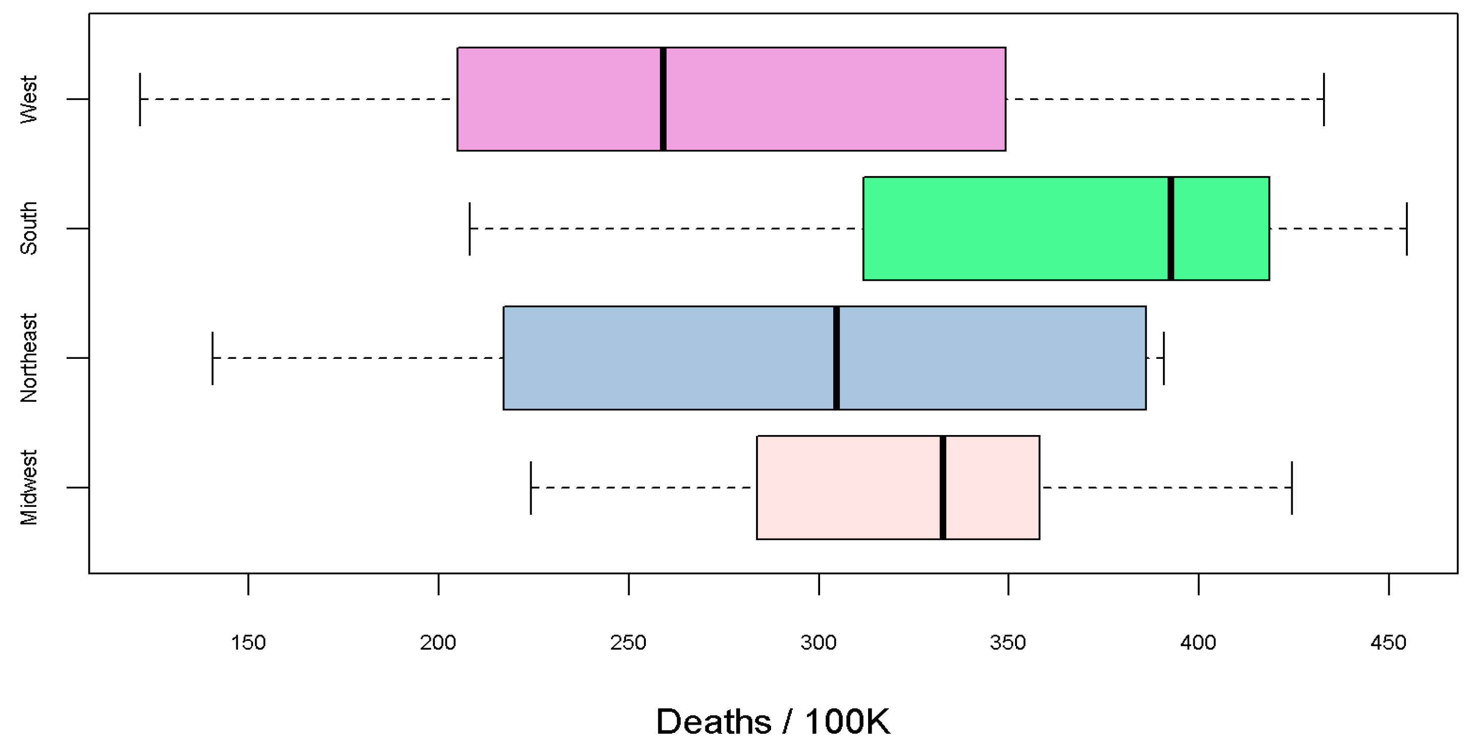
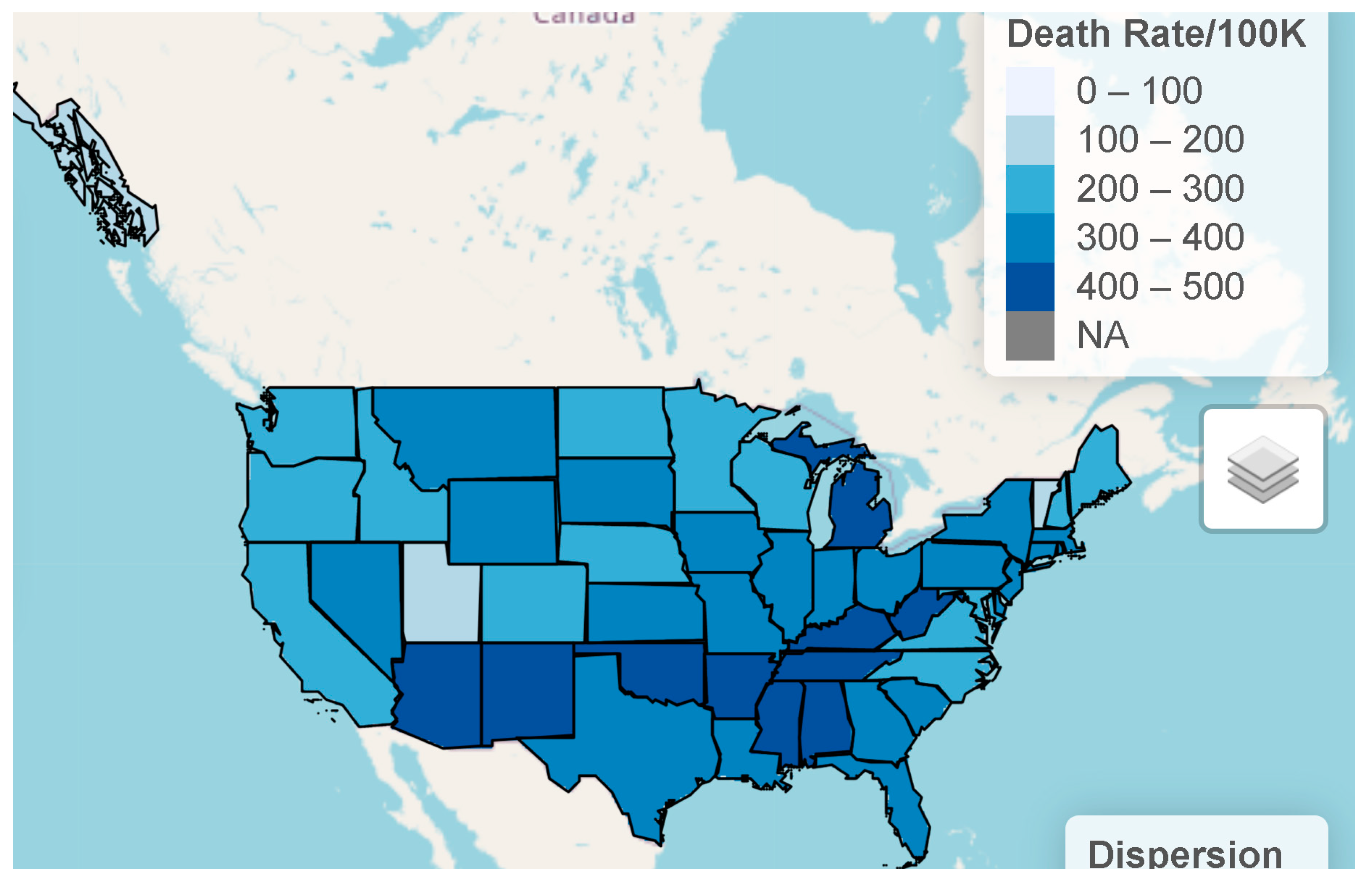
Rate 100K	320.740	86.544	335.487	121.480	454.672

for Total US and in

Table 2. Complementary index of the COVID-19 pandemic in overdispersed/volatile scenarios (1182 days).

Region	State	Deaths	Deaths/100K	nbiased	$\stackrel{-}{\mathrm{x}}$	$\stackrel{-}{\mathrm{x}}$biased	$\widehat{\mathit{\delta }}$	${\widehat{\mathit{\delta }}}_{\mathit{b}\mathit{i}\mathit{a}\mathit{s}\mathit{e}\mathit{d}}$	$\widehat{\mathrm{q}}$	$\widehat{\mathrm{q}}$biased	$\widehat{\mathrm{b}}$	$\widehat{\mathrm{b}}$biased
Midwest	IA	10,538	330	487	8.910	21.640	0.987	0.642	0.059	0.973	0.063	1.515
Midwest	IL	39,381	310	784	33.320	51.040	0.990	0.835	0.244	1.312	0.248	1.571
Midwest	IN	25,959	381	710	21.960	36.560	0.994	0.773	0.360	1.512	0.372	1.955
Midwest	KS	10,167	346	390	8.600	26.330	0.990	0.868	0.209	1.582	0.211	1.822
Midwest	MI	42,613	425	572	36.050	74.510	0.992	0.910	0.361	1.066	0.362	1.171
Midwest	MN	12,806	224	674	10.830	19.000	0.965	0.787	0.256	1.285	0.261	1.632
Midwest	MO	20,708	336	598	17.520	35.870	0.998	0.810	0.190	1.112	0.194	1.373
Midwest	ND	2232	287	399	1.890	5.600	0.945	0.556	0.187	1.452	0.222	2.612
Midwest	NE	4827	246	500	4.080	9.920	0.984	0.669	0.162	1.238	0.172	1.852
Midwest	OH	42,073	358	500	35.590	85.540	0.997	0.910	0.161	0.824	0.161	0.906
Midwest	SD	3214	359	348	2.720	9.260	0.954	0.880	0.094	1.590	0.094	1.807
Midwest	WI	16,486	280	911	13.950	18.270	0.977	0.630	0.148	1.290	0.164	2.047
Northeast	CT	11,034	305	483	9.340	22.910	0.980	0.805	0.112	1.134	0.113	1.409
Northeast	MA	21,035	301	678	17.800	36.910	0.999	0.716	0.262	1.415	0.278	1.975
Northeast	ME	2989	217	578	2.530	5.180	0.924	0.853	0.333	2.947	0.336	3.453
Northeast	NH	2972	214	545	2.510	5.790	0.979	0.836	0.130	2.095	0.131	2.506
Northeast	NJ	35,774	386	730	30.270	49.070	0.997	0.824	0.089	0.966	0.090	1.173
Northeast	NY	77,403	390	811	65.480	97.670	0.997	0.817	0.234	1.757	0.238	2.151
Northeast	PA	50,860	391	755	43.030	67.370	0.990	0.801	0.361	2.472	0.370	3.087
Northeast	RI	3897	355	407	3.300	9.630	0.973	0.836	0.024	2.129	0.024	2.546
Northeast	VT	910	141	314	0.770	2.900	0.919	0.783	0.219	1.855	0.223	2.369
South	AL	21,133	418	655	17.880	32.270	0.986	0.641	0.192	1.119	0.208	1.746
South	AR	13,062	431	779	11.050	16.810	0.967	0.885	0.271	2.035	0.273	2.300
South	DC	1392	208	412	1.180	3.390	0.841	0.776	0.375	2.023	0.389	2.607
South	DE	3371	335	513	2.850	6.570	0.943	0.848	0.032	0.877	0.032	1.035
South	FL	87,141	399	819	73.720	110.830	0.998	0.792	0.310	1.895	0.318	2.392
South	GA	42,348	393	715	35.830	65.490	0.997	0.676	0.236	1.271	0.255	1.879
South	KY	18,094	402	652	15.310	27.750	0.985	0.852	0.198	2.454	0.200	2.880
South	LA	18,136	392	695	15.340	26.100	0.976	0.649	0.103	1.180	0.109	1.819
South	MD	15,578	252	802	13.180	19.710	0.983	0.725	0.064	1.123	0.065	1.549
South	MS	13,097	444	610	11.080	21.730	0.972	0.652	0.054	1.209	0.055	1.853
South	NC	28,945	274	615	24.490	47.290	0.992	0.864	0.094	1.364	0.094	1.578
South	OK	18,147	455	176	15.350	118.400	0.999	0.715	0.598	1.898	0.648	2.653
South	SC	17,869	344	599	15.120	29.860	0.981	0.790	0.256	1.653	0.262	2.094
South	TN	28,113	403	703	23.780	40.040	0.996	0.898	0.202	2.382	0.202	2.654
South	TX	92,159	312	840	77.970	109.800	0.993	0.893	0.096	1.946	0.096	2.180
South	VA	23,718	274	825	20.070	28.820	0.985	0.912	0.020	1.175	0.020	1.288
South	WV	8083	453	656	6.840	12.750	0.969	0.753	0.305	1.335	0.318	1.772
West	AK	1441	196	298	1.220	4.960	0.951	0.882	0.411	1.560	0.415	1.769
West	AZ	29,852	411	564	25.250	53.510	0.992	0.723	0.089	1.079	0.091	1.493
West	CA	101,344	259	909	85.740	112.930	0.996	0.823	0.283	1.739	0.289	2.111
West	CO	14,194	244	773	12.010	18.450	0.979	0.719	0.126	1.064	0.132	1.480
West	HI	1758	121	346	1.490	5.110	0.900	0.850	0.084	1.358	0.084	1.597
West	ID	5463	287	553	4.620	9.950	0.943	0.906	0.520	1.682	0.523	1.856
West	MT	3705	335	529	3.130	7.020	0.925	0.698	0.379	1.645	0.414	2.357
West	NM	9164	433	828	7.750	11.090	0.923	0.816	0.292	2.072	0.296	2.539
West	NV	11,976	381	591	10.130	20.280	0.975	0.526	0.063	1.496	0.068	2.843
West	OR	8726	205	652	7.380	13.380	0.959	0.805	0.287	2.365	0.293	2.937
West	UT	5341	160	586	4.520	9.140	0.916	0.791	0.325	1.032	0.332	1.304
West	WA	16,013	207	611	13.550	26.840	0.979	0.750	0.210	1.239	0.216	1.651
West	WY	2023	349	170	1.710	12.320	0.968	0.751	0.055	1.078	0.056	1.436

for each US State

Daily COVID-19 fatality rates by county were obtained for 1 January 2020 through 12 May 2023 from the Centers for Disease Control and Prevention (CDC) via USA Facts [15], for 1182 days. The source of the data is https://usafacts.org/visualizations/coronavirus-covid-19-spread-map (accessed on 10 January 2020). County deaths were then aggregated by state level (and the District of Columbia) and transformed to reflect daily totals rather than cumulative totals. These data were then merged with US Census Bureau region and division assignments (https://www2.census.gov/geo/pdfs/maps-data/maps/reference/us_regdiv.pdf (accessed on 10 January 2020)) as well as estimated state populations for 2021 and state geographic shapefiles [15]. Deaths per 100,000 people were calculated using the aggregate fatalities and the population rate. R Statistical Software [16] was used to generate descriptive statistics, data tables, plots, and maps. Table 1 provides descriptive statistics for each of the variables in the data set. The average number of deaths by state was 21,554, and the median was 14,1494. The lowest number of deaths occurred in the state of Vermont (910) and the highest number of deaths in the state of California (101,344). The mean variance of deaths across the 1182 days was 3933, with the maximum variance belonging to the state of Florida (33,823) and the minimum variance belonging to Washington, D.C. On average, states experienced 18.235 deaths daily (median of 12.008), with Vermont reporting the fewest (0.770) and California again reporting the highest (85.739). Out of the 1182 days in the sample, the average number of non-zero was 600.98 (median of 610). The average overdispersion parameter (unbiased) was 0.971, while the average biased overdispersion parameter was 0.782. The average population of the states was 6.51 million (median of 4.51 million). On average, deaths per 100,000 people were 320.740 (median of 335.487). Surprisingly, Oklahoma experienced the highest death rate for this time (454.672 per 100,000 people), while Hawaii had the lowest death rate. The US Census Bureau assigns 12 states to the Midwest, 9 states to the Northeast, 17 states and D.C. to the South, and 13 states to the West.

Evaluating the death rate per 100,000 people by region illustrates a higher rate in the South region and lower rate in the West region (see Figure 5). Figure 5 displays comparative patterns of deaths among the four (east, middle, mountain, and western including Alaska and Hawaii) regions of the US. A non-parametric Kruskal–Wallis (KW) test confirmed the differences ($KW{\chi }_3^2=8.378,p=0.039$), and the Conover–Iman test found that the South and the West as well as the South and Northeast were statistically different (p = 0.003 and 0.0272, respectively). Insufficient power is available to investigate divisional differences, as one of the divisions contains only three states.

The parameter estimates were calculated for each state to estimate overdispersion. Table 2 details the estimates by region.

In Table 2, we note that $\widehat{\mathbf{đ}}$_biased is smaller than $\widehat{\mathbf{đ}}$, indicating that non-random (that is, biased) sampling has occurred. Figure 6 shows the graphs of reported deaths, the estimated death rate from those reports, and $\widehat{\mathbf{đ}}$_biased. These figures and all codes are available online at https://rpubs.com/R-Minator/Overdispersion (accessed on 10 January 2020).

Figure 6 and Figure 7 distinguish the actual number of deaths and deaths per 100,000 residents in the four regions of the US, respectively. In Figure 6, one can see that the three states with the most deaths from 1 January 2020 to 17 April 2023 were California (101,344), Texas (92,159), and Florida (87,141). The State of New York (77,403) was not very far behind. Figure 7 allows for a death rate comparison. There is a swath of states in the middle regions of the country, from Arizona through West Virginia, which experienced a higher number of deaths per 100,000 people than the rest of the country. The reason for this phenomenon is undetermined. Figure 8 displays the pattern of overdispersion across the four regions of the US according to the biased IRRP model (4). In Figure 8, we notice the highest overdispersion (biased) in Vermont (0.474) and the lowest in California (0.090), which is exactly opposite to the total number of deaths, where Vermont was lowest and California was highest. A correlation test indicates a strong negative correlation between biased overdispersion and the number of total deaths (r = −0.725, t₄₉ = −7.368, p < 0.001).

4. Conclusions

Wong [17] emphasized, in a recent working report, that discovery of knowledge is an integral part of efficiently handling the ongoing COVID-19 pandemic in nations around the world. Wong’s report was based on a magnificent attempt to collect, organize, analyze, and interpret data evidence on this global crisis. Wong enlisted the responses from healthcare sources, institutional sources, social institutions, educational institutions, economic sources, financial institutions, environmental sources, and information technology sectors to minimize the transmission of the virus. In the context of this, we examined and summarized pertinent findings on the ramifications of COVID-19 in the US. As much as the US has similarities with other nations, it also has its own uniqueness, as discovered. In fact, we learned in this article that some states within the US distinguished themselves from others. We notice an existence of heterogeneity according to the findings of several analyses in this article. A take-home message based on realizing this heterogeneity is the importance of creating a flexible but fair public health policy for the prevention of COVID-19 mortality.

References

- Shanmugam, R.; Fulton, L.; Betancourt, J.; Pacheco, G.J. Indexing Inefficacy of Efforts to Stop Escalation of COVID Mortality. Mathematics 2022, 10, 4646. [Google Scholar] [CrossRef]
- Shanmugam, R. Incidence rate restricted Poissonness. Sankhyā Indian J. Stat. Ser. B 1991, 531, 191–201. [Google Scholar]
- Shanmugam, R. Size biased incidence rate restricted Poissonness and its application in international terrorism. Appl. Manag. Sci. 1993, 7, 41–49. [Google Scholar]
- Pisl, V.; Vevera, J.; Štěpánek, L.; Volavka, J. Changes in ambulance departures for assault calls during COVID-19 pandemic restrictions. Aggress. Behav. 2023, 49, 76–84. [Google Scholar] [CrossRef]
- Siegel, R.L.; Miller, K.D.; Wagle, N.S.; Jemal, A. Cancer statistics, 2023. CA Cancer J. Clin. 2023, 73, 17–48. [Google Scholar] [CrossRef]
- Watson, A.M.; Haraldsdottir, K.; Biese, K.M.; Goodavish, L.; Stevens, B.; McGuine, T.A. The association of COVID-19 incidence with sport and face mask use in United States high school athletes. J. Athl. Train. 2023, 58, 29–36. [Google Scholar] [CrossRef]
- Udayana, S.; Dyah Wulan, S.R. The influence of local culture on mothers during pregnancy on stunting incidence. J. Posit. Psychol. Wellbeing 2022, 6, 2172–2180. [Google Scholar]
- Kersten, J.M.; van Veen, M.; van Houten, M.A.; Wieringa, J.; Noordzij, J.G.; Bekhof, J.; Kruizinga, M.D. Adverse effects of lockdowns during the COVID-19 pandemic: Increased incidence of pediatric crisis admissions due to eating disorders and adolescent intoxications. Eur. J. Pediatr. 2023, 182, 1137–1142. [Google Scholar] [CrossRef]
- Bisen, S.S.; Zeiser, L.B.; Boyarsky, B.; Werbel, W.; Snyder, J.; Garonzik-Wang, J.; Massie, A.B. Transplantation Amid a Pandemic: The Fall and Rise of Kidney Transplantation in the United States. Transplant. Direct 2023, 9, e1423. [Google Scholar] [CrossRef]
- Doti, J.L. A model to explain statewide differences in COVID-19 death rates. SSRN 2020, 3731803. [Google Scholar] [CrossRef]
- Riley, P.; Riley, A.; Turtle, J.; Ben-Nun, M. COVID-19 deaths: Which explanatory variables matter the most? PLoS ONE 2022, 17, e0266330. [Google Scholar] [CrossRef] [PubMed]
- Castro, M.C.; Gurzenda, S.; Turra, C.M.; Kim, S.; Andrasfay, T.; Goldman, N. Research notes: COVID-19 is not an independent cause of death. Demography 2023, 60, 343–349. [Google Scholar] [CrossRef] [PubMed]
- Almohaimeed, A.; Einbeck, J.; Qarmalah, N.; Alkhidhr, H. Using Random Effect Models to Produce Robust Estimates of Death Rates in COVID-19 Data. Int. J. Environ. Res. Public Health 2022, 19, 14960. [Google Scholar] [CrossRef]
- Shanmugam, R.; Fulton, L.; Ramamonjiarivelo, Z.; Betancourt, J.; Beauvais, B.; Kruse, C.S.; Brooks, M.S. A Report Card on Prevention Efforts of COVID-19 Deaths in US. Healthcare 2021, 9, 1175. [Google Scholar] [CrossRef] [PubMed]
- Shanmugam, R. Restricted prevalence rates of COVID-19′s infectivity, hospitalization, recovery, mortality in the USA and their implications. J. Healthc. Inform. Res. 2021, 5, 133–150. [Google Scholar] [CrossRef] [PubMed]
- Shanmugam, R.; Ledlow, G.; Singh, K.P. Predicting COVID-19 cases with unknown homogeneous or heterogeneous resistance to infectivity. PLoS ONE 2021, 16, e0254313. [Google Scholar] [CrossRef] [PubMed]
- Tian, T.; Tan, J.; Luo, W.; Jiang, Y.; Chen, M.; Yang, S.; Wang, X. The effects of stringent and mild interventions for coronavirus pandemic. J. Am. Stat. Assoc. 2021, 116, 481–491. [Google Scholar] [CrossRef]
- Stuart, A.; Ord, K. Kendall’s Advanced Theory of Statistics, Distribution Theory; John Wiley & Sons: Hoboken, NJ, USA, 2010; Volume 1. [Google Scholar]
- Shanmugam, R.; Singh, R. Testing of Poisson incidence rate restriction. Int. J. Reliab. Appl. 2001, 2, 263–268. [Google Scholar]
- USA Facts. US COVID-19 Cases and Deaths by State. 2022. Available online: https://usafacts.org/visualizations/coronavirusCOVID-19-spread-map (accessed on 2 November 2022).
- Fulton, L. Rpubs Code. 2022. Available online: https://rpubs.com/R-Minator/Ram22 (accessed on 2 November 2022).
- Wong, Y.L. COVID-Related Research on Singapore: A Review. Singapore: Academies. 2023. Available online: https://www.academia.sg/covid19-literature-review (accessed on 10 January 2020).
- Wu, R.; Pisani, D.; Donoghue, P.C. The unbearable uncertainty of panarthropod relationships. Biol. Lett. 2023, 19, 20220497. [Google Scholar] [CrossRef]
- Borisov, D. Mathematical modeling and multicriteria optimization of the ceramic indicators of the refractory linings of steel foundry ladles. J. Chem. Technol. Metall. 2023, 58, 208–216. [Google Scholar]
- Salekshahrezaee, Z.; Leevy, J.L.; Khoshgoftaar, T.M. The effect of feature extraction and data sampling on credit card fraud detection. J. Big Data 2023, 10, 6. [Google Scholar] [CrossRef]
- Chekouo, T.; Safo, S.E. Bayesian integrative analysis and prediction with application to atherosclerosis cardiovascular disease. Biostatistics 2023, 24, 124–139. [Google Scholar] [CrossRef] [PubMed]
- Ringwald, W.R.; Forbes, M.K.; Wright, A.G. Meta-analysis of structural evidence for the Hierarchical Taxonomy of Psychopathology (HiTOP) model. Psychol. Med. 2023, 53, 533–546. [Google Scholar] [CrossRef] [PubMed]