Abstract
This article constructs a behavioral financial model that provides feedback on both historical prices and company fundamentals without considering asset liquidation to discuss the long-term impact of investor sentiment and feedback trading on asset price fluctuations. The research conclusion shows that the abnormal volatility of asset prices is captured by the value effect, the cognitive bias effect, the sentiment shock effect, and the trading inductive effect. The value effect is the volatility of asset prices that is completely determined by fundamental factors; the higher the degree of cyclical fluctuations in fundamental factors, the higher the volatility of prices. The bias effect refers to investors’ misreading of basic information and trends in asset prices; the greater the instability of emotional shocks, the greater the abnormal volatility of asset prices. The trading inductive effect is also called the Keynes effect, which reflects the role played by rational traders.
MSC:
62P05
1. Introduction
Shiller (1981) and Le Roy and Porter (1981) [1,2] find that stock price volatility far exceeds the rational volatility boundary. Subsequent empirical studies have shown that the abnormal volatility of real asset prices is too high compared to the volatility of short-term real interest rates, consumption, and dividends, which is the so-called “volatility puzzle” (Campbell, 1999) [3]. As one of the three major aggregate anomalies, the explanation of this issue based on traditional rational theory is becoming increasingly weak. Behavioral finance theory has relaxed the assumption of investor rationality, opening up a new path for us to understand the “volatility puzzle”, greatly enhancing its explanatory power on financial anomalies compared to traditional theory. However, existing belief-based models (such as [4,5,6,7,8,9]) are mainly used to explain cross-sectional volatility. Although the mechanism of cross-sectional volatility can have an impact on the time series changes of aggregate levels, there are few belief-based models that can directly explain aggregate anomalies; this can only be seen in the dynamic general equilibrium theory model of the interaction of belief heterogeneous investors built by Dumas et al. (2009, referred to as DKU) [10]. Barberis et al. [11,12,13,14] introduce time-varying preference and non-consumption utility into standard CCAPM, capturing some factors that lead to abnormal volatility, but obviously not covering all bounded rationality. This paper attempts to construct a more general behavioral model to explain the anomalous volatility. Different from Shiller (1981) and Le Roy and Porter (1981) [1,2], who introduce the rational fluctuation boundary of asset prices from the effective market theory, we directly introduce the volatility boundary of asset prices from the cognitive deviation of investors. In addition, we distinguish the volatility caused by asset prices due to basic factors from the abnormal volatility caused by investors’ limited rationality.
The contributions of this article are as follows. Firstly, although asset prices can exhibit short-term momentum and long-term reversals in these models, they are mostly finite-period models and do not have generality. The long-term reversal of asset prices is due to the gradual disclosure or liquidation of public information. However, in reality, market information is generally noisy, making it difficult to find public information that accurately reflects the basic value of assets. Even if such public information exists in the market, due to investors’ irrational expectations, asset prices will still deviate from their basic values. For an asset that does not actually have any fundamental risk, but whose value is considered uncertain by noise traders, its price will still deviate from its fundamental value (De Long et al. [4]). Secondly, the assumption of liquidation is not realistic, as equity assets typically do not have a final liquidation period. Even under relaxed conditions, if only the next dividend is liquidated, investors still face capital gains and losses, and the asset prices of the next period are uncertain. For investors with lottery preferences, their primary focus is often not on dividends. Thirdly, regarding the manifestation of feedback trading, it mainly includes feedback between investor sentiment and asset prices, as well as feedback between investor sentiment and company fundamentals. However, this article combines the two. The investor sentiment of irrational investors not only responds to historical price changes, but also to fundamental factors of the company, which is consistent with the reality of the financial market and further promotes feedback theory. Fourthly, we discuss the long-term impact of investor sentiment and feedback trading on asset price volatility and obtain a closed-form solution with detailed economic implications for asset price volatility. The existing behavioral models explain financial market anomalies from two perspectives: beliefs and preferences (such as [9,11,12,13,14,15]). In fact, investors are influenced by a combination of beliefs and preferences in their decision-making process. We have added preference factors based on investor belief analysis. The results also well explain the formation and collapse of the bubble in the market.
To address the shortcomings of existing theories, we construct a more general infinite period model that does not include information disclosure or liquidation to cause mean reversals in asset prices. Our model is still a dual-factor model driven by a combination of external shocks and investor beliefs, with the difference being that we introduce more general feedback trading behavior to reflect investors’ beliefs. The psychological basis of feedback trading behavior and the market evidence are discussed in detail in the following section. There is currently no consistent definition of investor sentiment. Baker, M. et al. (2006) [16] provide two definitions of investor sentiment: (1) The tendency of investors to speculate, and the relative speculative demand driven by sentiment can cause asset price fluctuations; (2) the optimistic or pessimistic expectations about stocks. In fact, no matter how investor sentiment is defined, it will ultimately be reflected in the price, and the consequence is that asset prices deviate from their fundamental value. Therefore, we define sentiment shocks as changes in asset prices that cannot be explained by fundamental factors. In this way, we distinguish between rational and irrational components in price changes. Due to the interaction between investor sentiment and external shocks, the former has endogeneity, and the latter has exogeneity. In the absence of sentiment shocks, although investors themselves exhibit cognitive biases, this may not necessarily cause asset prices to deviate from their fundamental value. If investors can accurately observe basic information, their cognitive biases will only take effect driven by sentiment shocks. Sentiment shocks in the market are the result of the aggregation of numerous individuals, and asset price misalignment caused by sentiment shocks is universal [4]. The feedback trading behavior of investors has an amplifying effect on the fluctuations of external sentiment shocks.
The subsequent parts of this article are arranged as follows: The second part is a literature review and psychological evidence; the third part constructs a feedback trading model and discusses it from multiple aspects; the fourth part discusses the abnormal volatility of asset prices; and the fifth part is a summary and outlook of this article.
2. Literature Review and Psychological Evidence
The feedback theory of price to price is one of the most classic theories in the financial market, and as folk wisdom, it did not appear in academic journals at the earliest time (Shiller 2016 [17]). Investors buy when prices rise and sell when they fall. The theory of feedback trading has a long history, and the early Tulip Mania and the South China Sea company bubble are vivid manifestations of feedback trading. There have been two waves of research on feedback trading in the academic community. The first wave began in the 1990s, with representative scholars and classic works including DSSW (1990b) [4], Hong, H. (1999) [7], Barberis and Shleifer (2003) [18], etc. During this period, research mainly focused on theoretical models, depicting investors’ beliefs and decision-making processes through rigorous mathematical descriptions and reasoning. In 2014, Amromin and Sharpe (2014) [19] and Greenwood and Shleifer (2014) [20] successively provided survey data on future asset returns for investors in the real world. These data provide real and direct evidence for our research on the formation mechanism of investors’ beliefs, which attracted widespread attention from a large number of scholars and subsequently sparked a second wave of research on feedback trading. During this period, representative scholars and classic works include Barberis et al. [15,21], Adam et al. (2017) [22], Cassella and Gulen (2018) [23], Jin and Sui (2021) [24], and Liao et al. [9]. This kind of research attempts to reproduce investors’ real expectations through theoretical models, making abstract mathematical models match with real Market data. Subsequently, the academic community discovered that feedback trading was used to explain a series of financial anomalies. For empirical research, Sentana et al. 1992 [25] showed that feedback trading has an impact on both returns and volatility in stock prices. Koutmos [26] conducted a study on the stock markets of six major industrialized countries, finding that feedback trading is an important factor affecting short-term stock returns. The research of Nofsinger et al. [27] showed that the change of institutional investors’ shareholding has a strong correlation with the current stock excess return, and the positive feedback trading behavior of institutional investors and the price pressure effect of herding behavior have an impact on prices in each period. For theoretical modeling, Barberis et al. [21], Hu C.S. et al. [28], BGJS (2018) [8], and LPZ (2022) [9] believe that the demand of irrational investors is driven by investor sentiment, and the sentiment system is composed of historical price changes. The results show that this feedback trading behavior can explain a series of market anomalies. Moreover, feedback trading also exists between the secondary market and fundamental factors. There is a feedback loop between stock prices and company fundamentals (Hirshleifer et al., 2006 [29]), that is to say, the capital market not only has the function of price discovery, but also has the function of value creation. Higher stock prices mean that companies have better prospects than expected, thus leading to higher investment levels, and a rise in base value will in turn drive stock prices higher.
Feedback trading is supported by many psychological experiments. Andreassen, P. et al. 1990 [30] found that after presenting people with real stock price sequences, they were asked to trade in a simulated market. When prices showed a certain trend, they tended to use past price changes for trading. In the investor sentiment model constructed by BSV (1998) [5], which includes both representational and conservative biases, investors exhibit a characteristic of insufficient response to earnings announcements and similar events and overreact to events that exhibit consistent patterns. That is to say, investors tend to rely more on past price patterns when making decisions and assign less weight to recent events in decision-making, exhibiting the characteristics of feedback trading. BGJS (2018) [8] and LPZ (2022) [9] take expectation extrapolation as the psychological basis of feedback trading and discuss a series of empirical characteristics of bubbles using feedback trading.
The real feedback trading evidence is relatively more convincing. The Ponzi scheme is the most representative supporting evidence. In a Ponzi scheme, the scammers promise investors huge returns if they invest, but their investments are not really invested in any profitable assets. Instead, the scammers pay the next round of investors back to the previous round. Since investment cannot grow forever, the scam is doomed to an end. The scammers undoubtedly know this, and they may want to exit without paying the final round. In 1920, Charles Pang attracted 30,000 investors and issued notes worth USD 15 million within seven months. From 1996 to 1997, in Albania, seven Ponzi schemes accumulated USD 2 billion, equivalent to 30% of its GDP. Today, people are still enthusiastic about this kind of fraud. In 2008, Madoff’s Ponzi scheme involved up to USD 50 billion. Although there is no special design by the fraudster, the feedback loop that naturally appears in scams does indeed work. In the stock market, when the price rises many times, just like in the Ponzi scheme, investors gain profits from price changes, and the information about investing in the stock market and making money nearby stimulates investors’ emotions to rise, so as to join the stock market and further promote price changes.
From the early tulip boom to the South China Sea foam, the Internet foam, and the subprime mortgage crisis, it seems that people have not been able to escape the feedback loop of the stock market. People’s greed and fear in the formation and collapse of the bubble did not become a lesson to avoid the next struggle in the foam. The reason why investors cannot learn from the past bubble is that they may think that the situation in each period will be different. As time goes by, when a new bubble comes, investors may have forgotten about the old bubble (DSSW, 1990b) [4]. In fact, if we go back to each speculative event, we will find that there is no bubble that does not seem special at that time. It can be proved afterwards that a bubble is a bubble, and there will never be a special bubble. This kind of thing, determined by human nature, is very stable, and it has existed in the capital market for over 390 years. We can foresee that in the future, the feedback loop will still have a widespread impact on the stock market.
3. Model
Consider an economy where there are two types of assets on the market: risky assets and risk-free assets. The aggregate supply of risky assets is normalized to 1, and the supply of risk-free assets is fully elastic. For simplicity, without affecting the conclusion, we assume that risky assets do not distribute dividends and that investors’ gains and losses are fully reflected by changes in asset prices. The return on risk-free assets is 0. Next, we will complete the construction of the model through a series of assumptions.
Assumption 1.
Noise is ubiquitous in the market.
Due to the systematic nature of noise in the capital market, which can have a long-term impact on asset prices, the determining factors of asset prices are decomposed into two parts: one is the fundamental factor, which is the determination of the fundamental value of assets; another is investor sentiment, which is price misalignment relative to fundamental value.
Assumption 2.
Market trading occurs in discrete time.
The investor’s transaction occurs at the beginning of the period; the current period’s sentiment does not affect the current period’s price, but rather the next period’s price. Combined with Assumption 1, the price of period t reflects the fundamental factors of period t and the sentiment factors over the previous period. Hence, we can get the sentiment-price-driven equation:
For the convenience of handling, without affecting the conclusion, we assume that the price change and sentiment have the following relationship:
Among them, is the logarithm of the period price, denotes the logarithmic return during the period t. is the price growth rate determined by fundamental factors, is the price growth rate determined by sentiment factors during the t − 1 period, and is the reaction coefficient.
Assumption 3.
Investors are boundedly rational.
We use feedback trading to characterize the bounded rationality of investors. Therefore, the formation of investors’ t-period sentiment is influenced by the combined changes in current period prices and fundamental factors, resulting in the following basic form of the price-sentiment induction equation:
Specifically, we assume that there is a relationship between investor sentiment and returns as follows:
reflects investors’ cognitive bias towards fundamental information. The investor sentiment at the end of each period is influenced by fundamental factors that cannot be observed by investors in the current period’s price changes. This is an important difference from the feedback traders described in DSSW (1990b) [4], BGJS (2018) [8], and LPZ (2022) [9]. The feedback traders in these models only trade according to the price change during the previous period. In this model, investors not only trade according to the price change of the previous period, but also try to exclude the influence of fundamental factors in the price change, which is more consistent with the characteristics of “bounded rationality”. However, due to the incompleteness of the information and the bounded rationality of investors themselves, investors cannot accurately observe the fundamental information. Therefore, we have the following inference:
Inference 1.
When , investors provide accurate interpretation of fundamental information; when , investors overestimate fundamental information, which corresponds to overreaction about fundamental information; when , investors underestimate fundamental information, which corresponds to under-reaction about fundamental information.
Due to the discrete-time scenario, the fundamental information of the current period during the formation of sentiment has also been observed. Let us assume , which means that the higher the returns driven by sentiment factors during this period, the easier it is for investors to experience high sentiment. A combination of (2) and (4) can give
Let us set ; then, we have the following formula:
In the absence of external shocks, if investors accurately observe basic information, then price changes are completely driven by fundamentals. To illustrate this point, we assume that , , according to (6), . More generally:
From the above discussion, it can be seen that if investors accurately observe fundamental information (), even if they have the motivation to conduct feedback trading, the price will not deviate from the fundamental value in the absence of external shocks.
When , investors exhibit positive feedback trading; when , investors exhibit negative feedback trading. In this way, we have completed the characterization of bounded rationality investors with feedback trading characteristics. For such investors, we assume that they have CARA utility function: . Among them, is the risk aversion coefficient. Assuming that the asset return follows the normal distribution, the expected utility maximization is equivalent to the following formula (proof of Equations (9) and (10) in Appendix A):
If representative investors choose to hold units of assets to maximize expected utility, then the optimal asset holding amount is
Bounded rationality investors with feedback trading characteristics form expectations on prices through Formula (6); substituting Formula (6) into the above formula and simplifying, we obtain
Among them, , . Assuming that the number of investors is (11) quantified as 1, and the total supply of risky assets is 1, summing the above equation yields
From the above equation, it can be inferred that
It can be seen that the feedback trading coefficient used to describe bounded rationality investors comprehensively reflects investors’ risk aversion attitude, investors’ expectations of fundamental information, and the unexpected return rate over the previous period, which is consistent with DHS (1998) [6] and Barberis et al. 2001 [11], showing that the universality of feedback trading in characterizing investors’ bounded rationality. From Equation (12), it can be seen that there is a critical value that changes the feedback trading characteristics of investors. Investors based on feedback trading will adjust their behavioral characteristics according to conditions to maximize expected utility. Based on the above discussion, we have the following inference:
Inference 2.
Under different conditions, the market will exhibit different feedback trading characteristics.
Assumption 4.
Sentiment shocks are randomly generated in each period.
After assuming the characteristics of bounded rationality of investors, we take into account another factor, sentiment shock, to make the model dynamic. When sentiment shock is taken into account, Equation (6) becomes
where is the sentiment shock during period t, representing the changes in asset prices in the current period that cannot be explained by fundamental factors.
3.1. Single-Period Sentiment Shock
To analyze the impact of sentiment shock on asset prices, we consider the positive feedback scenario (). Assuming that investors can accurately observe fundamental information, if a sentiment shock occurs during the t + 1 period, it causes . So, from Equations (6) and (7), we can obtain . We define price misalignment as the deviation of price from the fundamental value: . Let us set and take different values of to observe the changes in price misalignment, as shown in Figure 1.
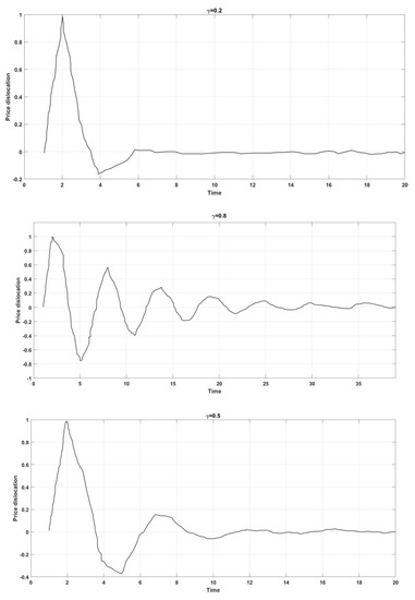
Figure 1.
Feedback coefficient and price dislocation (the parameter assignment here originates from Barberis (2018) [15]).
Figure 1 shows that as increases, the duration of the sentiment shock becomes longer, and vice versa. When a positive sentiment shock occurs, the price does not directly retreat to the fundamental value, but will overshoot below the fundamental value, and then reverse overshoot. The price adjusts in a wave-like manner around the fundamental value and ultimately converges to the fundamental value. This is different from the assumption that the adjustment mode of prices directly returns to fundamental value due to liquidation or information disclosure after external shocks [4,6,8].
The reason why price changes exhibit this characteristic is that when a sentiment shock occurs, such as a positive sentiment shock, abnormal price increases that cannot be explained by fundamental factors will drive investor sentiment to rise. For ease of understanding, we may consider trading volume as a proxy variable for sentiment. Compared to a situation without sentiment shock, high investor sentiment can induce them to trade more actively during the next period, resulting in a positive price misalignment. However, in cases of , the price dislocation decays over time. The adjustment of price misalignment is not achieved in one step, but rather decays in a “price-sentiment” spiral until the price returns to its fundamental value.
The impact of sentiment shocks on asset returns and volatility varies in the short and long terms. In the short term (see Figure 1), a positive sentiment shock can generate positive excess returns and trigger asset price volatility. In the long run, as asset prices gradually converge to their fundamental value, the impact of sentiment shocks gradually weakens, and assets do not exhibit price misalignment or abnormal volatility in the long run. We notice that price misalignment reached its maximum in the first period, but subsequent adjustments were not made at once. The time series of asset prices showed significant short-term positive correlation (momentum) and long-term negative correlation (reversal) at the statistical level.
Here, we do not consider the case of . In this situation, the sentiment shock of the current period will amplify over time and there will be no convergence trend, and asset prices will diverge, which is inconsistent with the actual observed situation.
More generally, if , assuming that a sentiment shock () occurs in the first period, then , . According to (6), it can be solved to obtain
When , in the case of positive feedback trading, we take a constant value for and different values for . The pattern of price dislocation is consistent with Figure 1. Assuming is a random variable with the same mean , we can obtain
When , the above equation is 0. That is, investors can accurately observe fundamental information, and a temporary sentiment shock will not have a permanent impact on asset prices. Only through feedback trading can such a simple trading strategy push asset prices back to their fundamental value. This is inconsistent with the commonly understood irrational trading behavior that only causes price misalignment. The reason why feedback trading behavior can cause mean reversals in prices is because investors accurately consider the influence of fundamental factors during each trading period. As investors conduct feedback trading, the impact of sentiment shocks gradually weakens and eventually converges to fundamental value. If , even without sentiment shock (), asset prices can still deviate from their fundamental value in the long term. If investors under-react to the latest fundamental information (), it will cause a positive price dislocation in asset prices. If they overreact to the latest fundamental information (), it will cause a negative price mismatch in asset prices. Due to investors’ conservatism bias, they often lack responsiveness to recent information (BSV, 1998; HS, 1999), resulting in asset premiums. This indicates that our consideration of investor information interpretation bias reflects the characteristics of the market well. Feedback trading behavior () will have a magnifying or narrowing effect on price misalignment.
3.2. Multiple Sentiment Shocks
The case of a single-period sentiment shock indicates that although feedback trading can affect asset returns and asset price volatility in the short term, this impact will tend to be weak in the long run. The assumption of a single period of sentiment shock is not general since noise is commonly present in the real market. To investigate the impact of more general feedback trading on asset price changes, we extended the model by assuming that sentiment shocks occur over multiple periods, letting be a random variable. The new sentiment shock may be the consequence of the addition of new noise traders, or the original investors may continue to show irrational tendencies. The investor sentiment that determines the t-period price can be further divided into the current period’s sentiment shock and the residual impact of previous sentiment on the current asset price, which we refer to as sentiment surplus. Combining Equation (6), the logarithmic price during period t can be expressed as
Among them, denotes the sentiment surplus, and
The above equation is a second-order linear homogeneous difference equation, and we can solve it to obtain
Furthermore, we assume that is an independent and identically distributed random variable with a mean of and a variance of . For sentiment shock , we also assume that this is an independent and identically distributed random variable with a mean of and a variance of . Based on the above assumptions, the unconditional expectation of the price dislocation during period t is
Taking the limit of Equation (20), we can obtain
The above equation indicates that in the presence of general sentiment shocks, asset prices can still deviate from fundamental value in the long run even when investors fully observe fundamental information. The degree of price misalignment is composed of the following four influencing factors: (1) the average level of sentiment shock in different periods ; the greater the intensity of sentiment shock, the greater the degree of price misalignment; (2) investors’ misinterpretation of information ; when investors do not respond adequately to recent information, there will be a premium on asset prices, and, conversely, asset prices will be discounted; (3) feedback on trading intensity ; the intensity of chasing up and selling assets will exacerbate price misalignment; (4) the average level of periodic changes in fundamental factors, investors’ information interpretation bias, and willingness to engage in feedback trading play a magnifying or narrowing role in this factor. Obviously, in multi-period scenarios, if emotional shocks are to have an impact on asset prices, then they must be widespread. DSSW (1990a) [31] construct a generational overlap model that includes rational investors and noise traders. The price dislocation level obtained by their model is directly proportional to the average optimism or pessimism of noise traders during different time periods. This is consistent with our first conclusion, indicating that the feedback trading model we construct from the interaction between sentiment and prices, which does not distinguish between rational and irrational levels, can better capture the long-term price characteristics of the market.
3.3. From First-Order Moment to Second-Order Moment
From Equation (16), it can be clearly seen that in the feedback system, the determining factors of asset prices can be further divided into the following: fundamental factors during each period; investors’ cognitive biases towards fundamental factors during each period; residual effects of previous sentiment shocks (sentiment surplus); and current sentiment shocks. We define the logarithmic return rate, , and combine Equations (6), (16) and (18) to obtain the period t’s logarithmic return rate:
Assuming that and are independent and identically distributed random variables, respectively, and independent of each other, from the above equation, we can obtain
Taking the limits on both sides of the above equation and organizing them gives
where , , .
The first item on the right side of Equation (24) refers to the asset price volatility completely determined by fundamental factors, which is the fundamental risk that we commonly encounter in behavioral financial models, measured by dividend volatility The higher the degree of cyclical fluctuation of fundamental factors, the higher the price volatility, which we call the “value effect of fundamental factors”. The second item on the right side is called the “cognitive bias effect”, which has two implications: investors’ misreading of basic information and misinterpretation of asset price trends. Hence, this term captures the third level of investor irrationality (Barberis 2018 [15]). The third item , known as the “sentiment shock effect”, includes two factors: investors’ willingness to engage in feedback trading and the sentiment shock level in the market. The last term is called the “trading inductive effect or Keynes effect”. The implication is very intuitive: investors are induced by sentiment shocks in different periods to conduct feedback trading, resulting in abnormal fluctuations in asset prices, which is consistent with the conclusion of DSSW (1990b) [4] and Hu C.S. et al. 2017 [28]. However, the direction of its impact on abnormal fluctuations in asset prices is not very clear. Based on the above analysis, we obtain inference 3:
Inference 3.
Cognitive bias effect, sentiment shock effect, and trading inductive effect are the causes of abnormal volatility of asset prices.
From inference 2, we know that the feedback trading behavior characteristics of investors () may change under certain conditions. In the case of positive feedback, we explore the relationship between the two parameters through numerical simulation, and the result is given in Figure 2. We can see that with the increase in feedback trading intensity, the Keynes effect weakens and thus has a significant inhibitory effect on asset price volatility. This conclusion is consistent with that of DSSW (1990b) [4] and Hu C.S. et al. 2017 [28]. Since the feedback trading strategy is conducted by an irrational investor, this agent is easily induced by smart rational speculators and becomes the target of exploitation. When the feedback trading intensity is weak, meaning that there is insufficient noise in the market, speculators will make noise and destabilize the market, thus making the price volatility very strong. As their feedback trading intensity is very significant, this creates an excellent profit opportunity for rational speculators. By trading inducement, irrational investors are attracted to buy assets recklessly, causing asset prices to rise rapidly. When prices are at their peak, they are often on the brink of collapse. Therefore, rational speculators sell assets at high prices in a timely manner, causing them to quickly switch from rising to falling. The process of price decline naturally manifests as a weakening of volatility. Hence, we have the following inference:
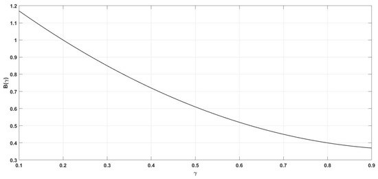
Figure 2.
Feedback trading intensity and the Keynes effect (the parameter assignment here originates from Barberis (2018) [15]).
Inference 4.
The impact of investor feedback on abnormal volatility of asset prices is linearly decreasing.
So far, in a two-asset environment, we have constructed an infinite feedback trading model through a series of assumptions about the market and investors, expanded the impact of the bounded rationality of investors with external shocks on asset prices from the first moment to the second moment, and applied the impact of investors’ under-reaction and over-reaction on asset prices to the total amount.
3.4. Further Discussion: Abnormal Fluctuations Introducing Time-Varying Preferences
Previous discussions have shown that a single period of sentiment shock will not cause the fluctuation of asset prices to exceed the upper limit of sentiment shock, and the maximum value of price misalignment is the price misalignment caused by sentiment shock. The reason is that we assume that the feedback trading coefficient can remain constant during every period. is a constant means that the feedback trading behavior of investors can keep stable compared to the price changes over the previous period. Corresponding to a price change, investors conduct feedback trading in a fixed pattern. However, according to the research of BHS (2001) [11], investors’ risk attitudes vary with time. When they make profits in the early stages, the private money effect will play a role, their risk aversion degree will decrease, and their willingness to conduct feedback transactions will increase. When they make losses in the early stages, the snake bite effect will play a role: their risk aversion degree will increase, and their willingness to conduct feedback transactions will decrease. Reflected on the feedback trading coefficient, it also has time-varying characteristics. Based on this, in the case of positive feedback, we assume that the feedback trading coefficient is a function of the previous period’s asset returns. Specifically, we assume that and the previous period’s asset returns have the following form:
We only consider the situation of a sentiment shock occurring during one period, and for the convenience of analysis, we assume that investors can accurately observe fundamental information. Assuming a sentiment shock occurs in the first period, then , . By combining Equation (6), we can obtain
Let us take , and calculate the price misalignment and feedback trading coefficient changes for each period. The results are shown in Figure 3.
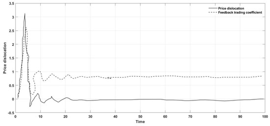
Figure 3.
Price misalignment and feedback trading coefficient.
The results here are consistent with the previous analysis of single-period sentiment shocks. The price adjustment is still not directly adjusted back to the fundamental value, but will overshoot, and the price fluctuation still shows a short-term positive correlation and a long-term negative correlation. The difference here from before is that price misalignment does not reach its maximum during sentiment shocks, but further expands after sentiment shocks, and prices can still exhibit short-term momentum effects after sentiment shocks. This is because, after taking into account the time-varying risk aversion of investors, a positive excess return of the previous period that cannot be explained by fundamentals can buffer investors’ future losses, thus reducing the degree of investors’ risk aversion. Investors will also more aggressively conduct feedback trading, and investors’ feedback trading coefficient may even be greater than 1. Furthermore, the feedback trading coefficient value here can ensure a positive value for the logarithm of price changes and effectively capture the private money effect and the snake bite effect. We have some technical skills in determining the values of and , as improper values can easily cause model divergence. However, this does not affect our intuitive understanding of the characteristics of price fluctuations when the feedback trading coefficient has time-varying characteristics. Here, we infer that can make the model converge, and decreases with ; that is, the greater the sentiment impact, the lower the investor’s sentiment for a long time after the bubble burst, and the lower the enthusiasm for trading.
The fact that the asset price can continue to deviate from the fundamental value after a sentiment shock means that the market is motivated to create a sentiment shock or a bubble, which is different from the situation where is a constant in a single period of sentiment shock. In the case of a constant feedback trading coefficient, since the maximum value of price dislocation is the impact of a sentiment shock on prices, prices will decline after a sentiment shock, and there is insufficient incentive to create a bubble at this time. Even if one can profit from it, they must wait for the price to fall after creating a positive shock, then buy at the lowest price and sell at the next high point. Such fluctuations make it almost impossible to profit from speculation. When the feedback trading coefficient is time-varying, the motivation to create a bubble is more feasible. After creating a sentiment shock, the feedback traders will reduce their risk aversion level due to the rise in price in the previous period, which will make investors more aggressive in feedback trading and promote further price dislocation. This is the mechanism of the Ponzi scheme described in the literature review in Section 2. This artificially created bubble has never stopped in history, which is vividly reflected in the early famous tulip boom, the South Sea Company’s foam, the Internet foam, and the subprime mortgage crisis.
4. Summary and Outlook
Based on the assumption that existing belief models have public information or liquidation periods, we construct an infinite-period model with typical feedback trading characteristics from the interaction between investor sentiment and price and study its impact on asset price volatility. Our model does not have public information that can bring asset prices back to their fundamental value, nor does it have a liquidation period, which is more in line with the characteristics of the real market and more general.
The findings of this paper are mainly as follows:
Firstly, through analysis, we have identified the root cause of abnormal fluctuations in asset prices: investors’ misreading of fundamental information and feedback trading behavior. This is because if investors can accurately observe fundamental information, for a single period of sentiment shock, feedback trading will not cause long-term price misalignment, but will gradually converge to its fundamental value. If investors have a bias in their interpretation of fundamental information, even if there is no sentiment shock, asset prices will still deviate from their fundamental value. This indicates that investors’ misreading of fundamental information and feedback trading behavior jointly constitute the root cause of abnormal volatility.
Secondly, we have identified the factors that affect asset price misalignment in the long term: the average level of sentiment shocks in different periods, investors’ misreading of fundamental information, willingness to engage in feedback trading, and the average level of cyclical changes in fundamental factors. The greater the intensity of sentiment shocks during different periods, the greater the degree of price misalignment. When investors do not respond adequately to recent information, there will be a premium on the asset, and conversely, the asset will be discounted. If investors’ willingness to engage in feedback trading increases, the price misalignment also increases accordingly. The higher the average level of periodic changes in fundamental factors, the greater the degree of price misalignment.
Thirdly, by introducing feedback trading, a common feature of the market, we directly introduce the fluctuation boundary of asset prices from the cognitive bias of investors and well define abnormal volatility. According to the traditional rational theory, asset prices are completely driven by fundamental factors, and asset price volatility should be captured by the value effect determined by fundamental factors. However, under the constraints of investors’ limited rationality, the volatility of asset prices will exceed the rational volatility boundary and produce abnormal volatility. The abnormal volatility of asset prices is captured by three effects: the cognitive bias effect, the sentiment impact effect, and the trading inducement effect. The cognitive bias effect reflects the investors’ misreading of basic information and price trends; the sentiment impact effect reflects the different periods of sentiment impact due to the instability of the influence of the asset price’s abnormal volatility; and the trading inducement effect reflects the investors by sentiment impact-induced feedback trading caused by abnormal volatility.
The research presented in this paper can be further expanded. We introduce time-varying preferences in the fourth part to study anomalous volatility, which makes the feedback trading coefficient time-varying. For small shocks, it is reasonable to assume that the feedback trading coefficient is a constant. However, in the face of big shocks, such as economic disasters, it will have a huge impact on asset prices. From our tentative discussion, we can see that the time-varying feedback trading coefficient can better reflect the characteristics of market price changes. Therefore, introducing cyclical external shocks and time-varying feedback trading coefficients is an important direction for future research in this article.
Author Contributions
Conceptualization, C.C.; methodology, C.H.; software, L.W. All authors have read and agreed to the published version of the manuscript.
Funding
This research was funded by National Natural Science Foundation of China, grant number 71671134 and China Postdoctoral Science Foundation, grant number 2023M731385.
Data Availability Statement
Not applicable.
Conflicts of Interest
The authors declare no conflict of interest.
Appendix A
Proof of Equations (9) and (10).
Due to our assumption that investors have a CARA utility function, we can obtain the optimal demand for risky assets based on the ideas of Hu C.H. et al. (2017) [28] and Barberis (2018) [15]:
The Utility maximization problem of investors can be converted to
In t − 1, the expected wealth is , and the conditional variance of the final wealth is . From this, we can obtain
By taking the first derivative of , we can obtain Equation (9).
Then, if we substitute Equation (6) into Equation (9) and combine market clearing criterion , we can obtain Equation (10). □
References
- Shiller, R.J. The Use of Volatility Measures in Assessing Market Efficiency. J. Financ. 1981, 36, 291–304. [Google Scholar]
- Le Roy, S.; Porter, R. The Present-Value Relation: Tests Based on Implied Variance Bounds. Econometrica 1981, 49, 555–574. [Google Scholar] [CrossRef]
- Campbell, J.Y.; Shiller, R.J. The Dividend-Price Ratio and Expectations of Future Dividends and Discount Factors. Rev. Financ. Stud. 1999, 1, 195–228. [Google Scholar] [CrossRef]
- De Long, J.B.; Shleifer, A.; Summers, L.H.; Waldman, R.J. Positive Feedback Investment Strategies and Destabilizing Rational Speculation. J. Financ. 1990, 45, 375–395. [Google Scholar] [CrossRef]
- Barberis, N.; Shleifer, A.; Vishny, R. A Model of Investor Sentiment. J. Financ. Econ. 1998, 49, 307–343. [Google Scholar] [CrossRef]
- Daniel, K.; Hirshleifer, D.; Subrahmanyam, A. Investor Psychology and Security Market under and Overreactions. J. Financ. 1998, 53, 1839–1886. [Google Scholar] [CrossRef]
- Hong, H.; Stein, J.C. A Unified Theory of Underreaction, Momentum Trading, and Overreaction in Asset Markets. J. Financ. 1999, 54, 2143–2184. [Google Scholar] [CrossRef]
- Barberis, N.; Greenwood, R.; Jin, L.; Shleifer, A. Extrapolation and Bubbles. J. Financ. Econ. 2018, 129, 203–227. [Google Scholar] [CrossRef]
- Liao, J.; Peng, C.; Zhu, N. Extrapolative Bubbles and Trading Volume. Rev. Financ. Stud. 2022, 35, 1682–1722. [Google Scholar] [CrossRef]
- Dumas, B.; Kurshev, A.; Uppal, R. Equilibrium Portfolio Strategies in the Presence of Sentiment Risk and Excess Volatility. J. Financ. 2009, 64, 579–629. [Google Scholar] [CrossRef]
- Barberis, N.; Huang, M.; Santos, T. Prospect Theory and Asset Prices. Q. J. Econ. 2001, 116, 1–53. [Google Scholar] [CrossRef]
- Barberis, N.; Huang, M. Mental Accounting, Loss Aversion, and Individual Stock Returns. J. Financ. 2001, 56, 1247–1292. [Google Scholar] [CrossRef]
- Barberis, N.; Huang, M. Preferences with Frames: A New Utility Specification that Allows for the Framing of Risks. J. Econ. Dyn. Control 2009, 33, 1555–1576. [Google Scholar] [CrossRef]
- Barberis, N.; Huang, M.; Thaler, R. Individual Preferences, Monetary Gambles, and Stock Market Participation: A Case for Narrow Framing. Am. Econ. Rev. 2006, 96, 1069–1090. [Google Scholar] [CrossRef]
- Barberis, N. Psychology-Based Models of Asset Prices and Trading Volume. In Handbook of Behavioral Economics: Applications and Foundations 1; Elsevier: Amsterdam, The Netherlands, 2018; Volume 1, pp. 79–175. [Google Scholar]
- Baker, M.; Wurgler, J. Investor sentiment and the cross-section of stock returns. J. Financ. 2006, 61, 1645–1680. [Google Scholar] [CrossRef]
- Shiller, R. Irrational Exuberance; China Renmin University Press: Beijing, China, 2016. [Google Scholar]
- Barberis, N.C.; Shleifer, A. Style Investing. J. Financ. Econ. 2003, 68, 161–199. [Google Scholar] [CrossRef]
- Amromin, G.; Sharpe, S.A. From the Horse’s Mouth: Economic Conditions and Investor Expectations of Risk and Return. Manag. Sci. 2013, 60, 845–866. [Google Scholar] [CrossRef]
- Greenwood, R.; Hanson, S. Waves in Ship Prices and Investment. Q. J. Econ. 2014, 130, 55–109. [Google Scholar] [CrossRef]
- Barberis, N.; Greenwood, R.; Jin, L.; Shleifer, A. X-CAPM: An Extrapolative Capital Asset Pricing Model. J. Financ. Econ. 2015, 115, 1–24. [Google Scholar] [CrossRef]
- Adam, K.; Marcet, A.; Beutel, J. Stock Price Booms and Expected Capital Gains. Am. Econ. Rev. 2017, 107, 2352–2408. [Google Scholar] [CrossRef]
- Cassella, S.; Gulen, H. Extrapolation Bias and the Predictability of Stock Returns by Price-Scaled Variables. Rev. Financ. Stud. 2018, 31, 4345–4397. [Google Scholar] [CrossRef]
- Jin, L.J.; Sui, P. Asset Pricing with Return Extrapolation. J. Financ. Econ. 2021, 2021, e3045658. [Google Scholar] [CrossRef]
- Sentana, E.; Wadhwani, S. Feedback Traders and Stock Return Autocorrelations: Evidence from a Century of Daily Data. Econ. J. 1992, 102, 415–425. [Google Scholar] [CrossRef]
- Koutmos, G. Feedback Trading and the Autocorrelation Pattern of Stock Returns: Further Empirical Evidence. J. Int. Money Financ. 1997, 16, 625–636. [Google Scholar] [CrossRef]
- Nofsinger, J.; Sias, R. Herding and Feedback Trading by Institutional and Individual Investors. J. Financ. 1999, 54, 2263–2295. [Google Scholar] [CrossRef]
- Hu, C.S.; Peng, Z.; Chi, Y.C. Feedback trading, Trading inducement and Asset price behavior. Econ. Res. J. 2017, 5, 189–202. [Google Scholar]
- Hirshleifer, D. Feedback and the Success of Irrational Investors. J. Financ. Econ. 2006, 81, 311–338. [Google Scholar] [CrossRef]
- Andreassen, P.; Kraus, S. Judgmental extrapolation and the salience of change. J. Forecast. 1990, 9, 347–372. [Google Scholar] [CrossRef]
- De Long, J.; Shleifer, A.S.; Waldman, R. Noise trader risk in financial markets. J. Political Econ. 1990, 98, 703–738. [Google Scholar] [CrossRef]


Disclaimer/Publisher’s Note: The statements, opinions and data contained in all publications are solely those of the individual author(s) and contributor(s) and not of MDPI and/or the editor(s). MDPI and/or the editor(s) disclaim responsibility for any injury to people or property resulting from any ideas, methods, instructions or products referred to in the content. |
© 2023 by the authors. Licensee MDPI, Basel, Switzerland. This article is an open access article distributed under the terms and conditions of the Creative Commons Attribution (CC BY) license (https://creativecommons.org/licenses/by/4.0/).