Communication

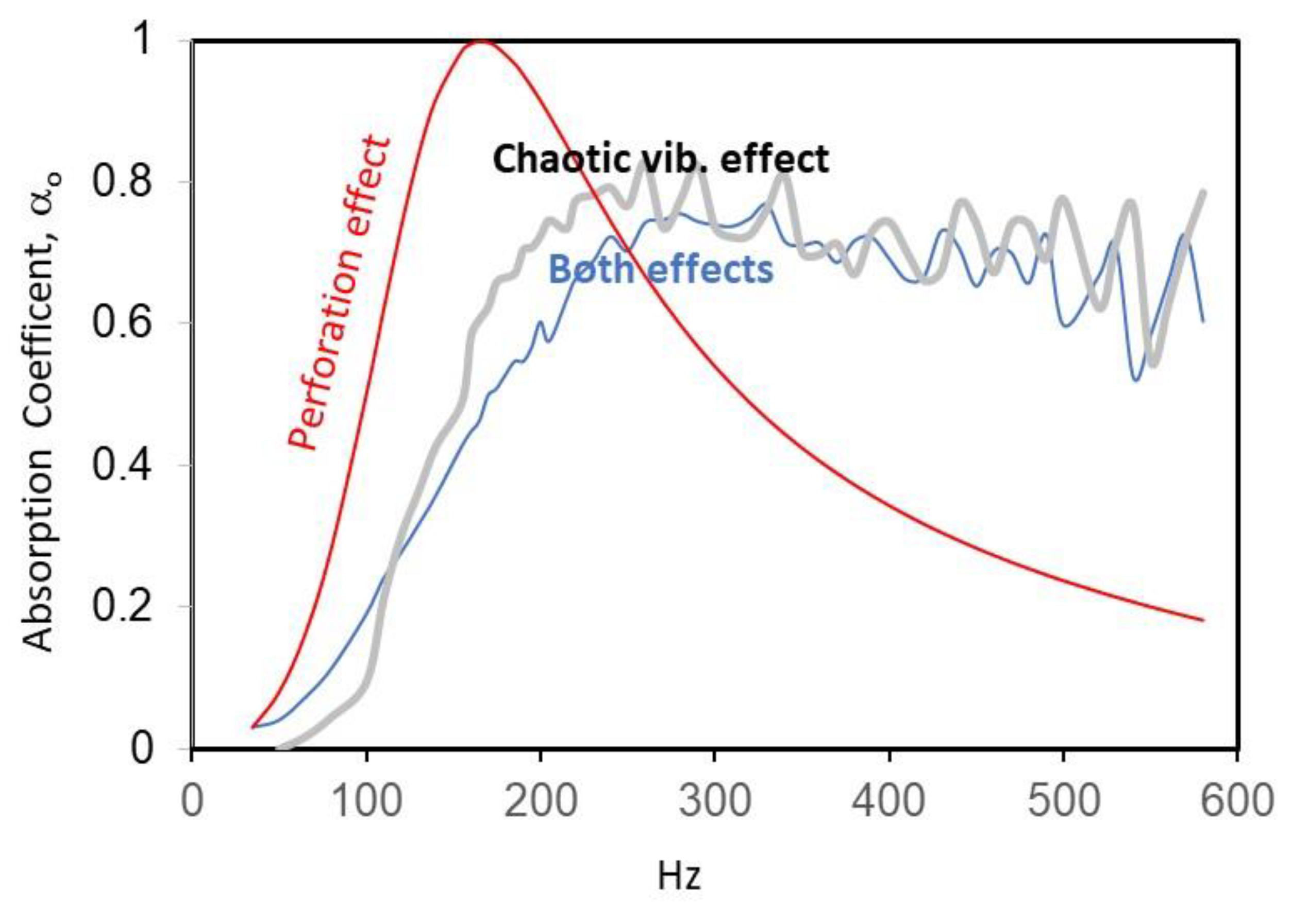
Chaotic Vibration and Perforation Effects on the Sound Absorption of a Nonlinear Curved Panel Absorber

Department of Architecture and Civil Engineering, City University of Hong Kong, Tat Chee Avenue, Kowloon 852, Hong Kong
Mathematics 2023, 11(14), 3178; https://doi.org/10.3390/math11143178
Submission received: 29 May 2023 / Revised: 12 July 2023 / Accepted: 17 July 2023 / Published: 20 July 2023
(This article belongs to the Special Issue Mathematical Modeling and Simulation of Oscillatory Phenomena)

Abstract

:
This study is the first to investigate the effect of chaotic vibration on the sound absorption of a curved perforated panel. Previous studies on the effect of nonlinear vibration on the sound absorption of a panel absorber have focused on periodic responses only. In this study, a sound absorption formula was derived by considering the panel impedance and perforation impedance. The numerical integration method was adopted to generate various chaotic vibrational responses, which were used to compute the corresponding sound absorptions. Several interesting findings that have never been observed in any previous studies on acoustic absorption were derived. First, in the chaotic and highly nonlinear cases, as the excitation frequency increased, the corresponding response frequencies decreased. This was opposite to the typical trend in linear cases, in which higher excitation frequencies corresponded to higher response frequencies. Second, in chaotic cases, absorption mainly occurred due to panel vibration effects. This is also in stark contrast to the findings of studies on perforated vibrating panels, in which the absorption effect mainly originates from perforations. Additionally, the absorption bandwidths are much wider and can shift to higher frequencies; however, the peak absorption coefficients were approximately 20% lower than in the case of the perforation effect only. Third, in the quasi-chaotic case, the absorption curve in the case of the perforation effect plus the vibration effect was between the absorption curves of the perforation effect only and the perforation effect plus the vibration effect.

1. Introduction

In recent decades, various studies have investigated the nonlinear vibration and absorption, insulation, and propagation of sound (e.g., [1,2,3,4,5,6,7,8,9,10,11,12,13,14]). However, most of these works have focused on only a single research area (e.g., nonlinear vibration or acoustics). Gorain and Padmanabhana [1] proposed a new broadband acoustic metamaterial absorber made of polyurethane foam and small-size tuned resonators, which offered good low-frequency noise attenuation. Rahman and Hasan [2] studied a second approximate solution of nonlinear jerk equations (an example of third-order differential equations), which was obtained using a modified harmonic balance method. It was argued that this method could simplify the solution of nonlinear differential equations due to its generation of fewer nonlinear equations in the harmonic balance process. Ding et al. [3] developed a model of the chaotic behavior of an axially moving viscoelastic tensioned beam under external harmonic excitation. The nonlinear integral-partial-differential governing equation included a material derivative in the viscoelastic constitution relation and finite axial support rigidity. The numerical solutions of these nonlinear governing equations were obtained using Galerkin truncation and Runge–Kutta time discretization. Hirwani et al. [4] studied the nonlinear frequency responses of laminated carbon/epoxy composite curved shell panels. Their model, which was derived from two higher-order theories and Green Lagrange nonlinear strains, included all of the nonlinear higher-order strain terms in the formulation to achieve generality. Razzak et al. [5] adopted a modified multiple-time-scale method to solve strongly nonlinear forced vibration systems. The unique strength of this method was that only the first-order approximation was used, thus reducing complexity and avoiding tedious steps. Ghafouri et al. [6] investigated the sound propagation of three-dimensional (3D) sandwich panels and the influence of a re-entrant auxetic core. They adopted an analytical strategy to investigate the exact effect of using 3D-RACS to determine the sound transmission loss (STL) and the coefficient of the sandwich panel. The dynamic equations of the fluid–structure interaction were solved analytically based on the state vector method. Their sandwich model improved the STL characteristics of the system with a complex core model. Ghassabi et al. [7] presented a new model of wave propagation through functionally graded doubly curved, thick nanocomposite structures. They focused on the properties of nanocomposite media. The state vector solution was used to solve the 3D equations of motion. The results showed that carbon nanotubes enhanced the sound insulation properties of doubly curved structures. Ghafouri et al. [8] investigated STL on a doubly curved shell with a 3D re-entrant auxetic cellular structure. Based on the 3D elasticity theory and using the state space method, they developed a theoretical approach to study the effects of core parameters on STL. It was found that the core’s substantial effect was crucial in reducing the curvature frequency. In the mass control domain, adding the core into the structure significantly increased the STL and affected the coincidence frequency. Refs. [7,8] represent two of the limited number of studies on the sound insulation properties of curved structures. Zarastvand et al. [9] presented a good review of the sound propagation prediction for plate structures, including more than 200 studies on acoustic performance, with an emphasis on material types, such as composites, isotropic and functionally graded materials, and sandwich plates. The review also focused on the optimization and control of sound transmission through plate structures. It was concluded that although numerical and analytical techniques had some ability to predict the acoustic performance of various structures, they did not reach the accuracy of the measured data.
In fact, there has been no research into the effect of chaotic vibrations on the absorption performance of a panel absorber. Moreover, few studies on nonlinear absorbers and nonlinear structural-acoustic problems have been conducted [15,16,17,18,19,20,21,22,23,24,25,26]. Thus, only a few relevant studies are mentioned here. Chiang and Choy [15] investigated the acoustic performance of a microperforated panel absorber array in a nonlinear regime. The absorber array was constructed from three parallel-arranged absorbers with different cavity depths. It was found that the absorption performance depended on the incident sound pressure in the region of 100 dB and above. Absorber arrays in some nonlinear cases outperformed those in linear cases because of an improvement in the equivalent acoustic impedance matching with ambient air. Motaharifar et al. [16] analyzed the nonlinear vibration of an isotropic cracked plate interacting with an air cavity. Based on the von Karman theory, they developed nonlinear governing equations for a cracked plate–cavity system. These nonlinear responses were generated from governing equations using the Euler equation along with the Galerkin method and the variational iteration method. The effects of the length, angle, position, and cavity depth were studied. It was found that the crack angle was the most influential parameter on the frequency ratio. Lee et al. [17] studied the sound absorption of a nonlinearly vibrating curved panel backed by a cavity. A curved panel was considered because the overall absorption bandwidth could be designed and optimized by appropriately adjusting the panel’s curvature to tune resonant behaviors. Lee [18] developed a model on the effect of leakage on the sound absorption of a nonlinear perforated absorber. It was found that leakages could improve the low-frequency average absorption but slightly degrade the medium-frequency average absorption. However, none of the aforementioned works have considered both the chaotic-vibration effect and sound absorption together. This study is the first to investigate the chaotic vibration of a structural acoustic system.

2. Theory

Figure 1 shows the nonlinear curved perforated absorber that is proposed in this study, the main theme of which is chaotic vibration. In practice, some inevitable slipping effects at the panel edges could induce a deviation in the natural frequency responses. In order to reduce the slipping effects on the dynamic measurement, the boundary portion of the panel could be stiffened with thick metal fixtures and stiff bolts [27]. It was mentioned in [28] that when the cavity length/width ratio was high enough (i.e., 4.25). the lowest two cavity resonances affected the lowest two structural resonant responses. Hence, this could be a reference for designing cavity dimensions. According to many previous studies (e.g., [29,30,31,32]), the cavity depth ranges from 100 mm to 500 mm; thick metal or concrete panels should be used as rigid boundaries. In many previous studies, the absorption frequency ranges were designed between 100 Hz and 600 Hz.
The main theme of this paper is chaotic vibration. The next section presents some results pertaining to the system configurations that were used for triggering chaotic vibrations. First, however, the impedance of the nonlinear panel was derived. According to [17], the governing equation for a large-amplitude vibration is given as follows. Note that (1) it is assumed in [17] that the flexural bending along the width is negligible, and (2) this model considers the average cavity depth D.
ρ p d 2 w d t 2 + C p d w d t + E I d 4 w d x 4 = E b h a d 2 ( w + w o ) d x 2 0 a d w d x d w o d x + 1 2 d w o d x 2 d x = F p
where w is the transverse displacement; w o is the pre-set initial displacement profile (i.e., s i n ( π a x ) ); E is Young’s modulus; ρ p is the panel surface density; C p is the panel damping coefficient; a, b, h are the panel width, length, and thickness, respectively; F p is the external force acting on the panel.
The physical transverse displacement could be expressed in terms of modal displacements as:
w = A 1 ϕ 1 + A 2 ϕ 2 + A 3 ϕ 3 + + A N ϕ N = n = 1 N A n ϕ n  
where A n and ϕ n are the nth modal amplitude and mode shape; N is the number of modes used; for the simply supported case, ϕ n = s i n ( n π a x ) . In this section, the equations for three structural modes are presented (i.e., N = 3. In the next section, the convergence study checks whether the three-mode approach is accurate enough). When Equation (2) is placed into (1) the modal decomposition process can be undertaken (i.e., multiplying ϕ n and taking integration).
0 a ϕ 1 ϕ 1 d x ρ p d 2 A 1 d t 2 + 2 ρ p ξ ω   d A 1 d t + E I A 1 E b h a 0 a d ϕ 1 d t d ϕ 1 d t d x A o 2 A 1 E b h a 3 2 0 a d ϕ 1 d x d ϕ 1 d x d x 0 a d 2 ϕ 1 d x 2 ϕ 1 d x A o A 1 2 + 1 2 0 a d ϕ 2 d x d ϕ 2 d x d x 0 a d 2 ϕ 2 d x 2 ϕ 2 d x A o A 2 2 + 1 2 0 a d ϕ 3 d x d ϕ 3 d x d x 0 a d 2 ϕ 1 d x 2 ϕ 1 d x A o A 3 2 + 1 2 0 a d ϕ 1 d x d ϕ 1 d x d x 0 a d 2 ϕ 1 d x 2 ϕ 1 d x A 1 3 + 1 2 0 a d ϕ 2 d x d ϕ 2 d x d x 0 a d 2 ϕ 1 d x 2 ϕ 1 d x A 1 A 2 2 + 1 2 0 a d ϕ 3 d x d ϕ 3 d x d x 0 a d 2 ϕ 1 d x 2 ϕ 1 d x A 1 A 3 2                          = 0 a F p ϕ 1 d x
0 a ϕ 2 ϕ 2 d x ρ p d 2 A 2 d t 2 + 2 ρ p ξ ω   d A 2 d t + E I A 2     E b h a [ 0 a d ϕ 1 d x d ϕ 1 d x d x 0 a d 2 ϕ 2 d x ϕ 2 d x A o A 1 A 2     + 1 2 0 a d ϕ 1 d x d ϕ 1 d x d x 0 a d 2 ϕ 2 d x 2 ϕ 2 d x A 1 2 A 2     + 1 2 0 a d ϕ 2 d x d ϕ 2 d x d x 0 a d 2 ϕ 2 d x 2 ϕ 2 d x A 2 3     + 1 2 0 a d ϕ 3 d x d ϕ 3 d x d x 0 a d 2 ϕ 2 d x 2 ϕ 2 d x A 3 2 A 2 ]    = 0 a F p ϕ 2 d x
0 a ϕ 3 ϕ 3 d x ρ p d 2 A 3 d t 2 + 2 ρ p ξ ω   d A 3 d t + E I A 3 E b h a [ 0 a d ϕ 1 d x d ϕ 1 d x d x 0 a d 2 ϕ 3 d x ϕ 3 d x A o A 1 A 3 + 1 2 0 a d ϕ 1 d x d ϕ 1 d x d x 0 a d 2 ϕ 3 d x 2 ϕ 3 d x A 1 2 A 3 + 1 2 0 a d ϕ 2 d x d ϕ 2 d x d x 0 a d 2 ϕ 3 d x ϕ 3 d x A 2 2 A 3 + 1 2 0 a d ϕ 3 d x d ϕ 3 d x d x 0 a d 2 ϕ 3 d x 2 ϕ 3 d x A 3 3 = 0 a F p ϕ 3 d x
where F p = λ   ρ p   g   sin ω t ; ω is the excitation frequency (radian per second); g = 9.81 ms−2; λ is a dimensionless excitation parameter; ξ is the damping ratio.
The physical transverse displacement could be expressed in terms of modal displacements. The modal displacement and velocity responses of the panel were obtained using the Runge–Kutta numerical integration function in MathCad to solve Equations (3)–(5) (MathCad is software for engineering and scientific computations). The MathCad formats required for the Runge–Kutta numerical integration are shown below. A function must be defined in MathCad and assigned differential equations before the acoustic impedance of the nonlinear panel is considered.
P D E t , q   = q 2 d 2 A 1 d t 2 q 4 d 2 A 2 d t 2 q 6 d 2 A 3 d t 2
q = q 1 q 2 q 3 q 4 q 5 q 6 = A 1 d A 1 d t A 2 d A 2 d t A 3 d A 2 d t
where PDE(t,q) is a MathCad function representing the differential equations in Equations (3)–(5). The second derivatives in (6) could be expressed in terms of the modal displacements and velocities using Equations (3)–(5). The general concept and procedures of the Runge–Kutta method are shown in Appendix A.
Then, the acoustic impedance of the nonlinear panel could be considered:
Z p = R p + i I p
R p = 2 ρ p ξ ω
where Rp and Ip are the real and imaginary parts; i = 1 . The real part was the damping term in the system. The imaginary part Ip, which represented the mass and stiffness reactance, could be obtained by the following equations.
I p = Z p 2 R p 2
Z p = F p ρ a c a n = 1 N d A n d t
where ρa and ca are the air density and sound speed, respectively. Next, the impedance of the micro-holes on the panel, which could be found in [30,31,32], was considered, which is shown in the following equations:
R m = 0.147 h σ   d 2 9 + 100 d 2 f 32 + 1.768 f d 2 h
I m = 1.847 f h σ 1 + 1 9 + 50 d 2 f + 0.85 d h
where Rm and Im are the real and imaginary parts of the impedance; d is the hole diameter; h is the panel thickness; σ is the hole ratio; f is the excitation frequency (Hz). The overall acoustic impedance of the curved panel absorber could be considered to be analogous to that of the electrical circuit. This was given by the following equation:
Z o = Z p Z m Z p + Z m + Z c
Z c = i ρ a ω   c o t ω c a D
where Zm is the impedance of the micro-holes, which is equal to Rm + i Im; Zc is the cavity impedance; D is the cavity depth; Ca is sound speed; ω is the excitation frequency (radian/s). Finally, the absorption coefficient of the nonlinear curved absorber could be computed using the following formula,
α o = 4 R e Z o 1 + R e Z o 2 + I m Z o 2

3. Results and Discussion

In the numerical simulation cases considered in this section, the material properties were set as follows: Young’s modulus E = 7 × 10¹⁰ N/m2, Poisson’s ratio ν = 0.3, and mass density ρ = 2700 kg/m3. The sound speed and air density were 340 m/s and 1.2 kg/m3, respectively. Table 1 shows the results of a convergence study for various excitation frequencies, magnitudes, and damping ratios. The initial center of deflection was 10 mm, and the panel thickness was 2 mm. The length and width were 400 mm and 300 mm, respectively. The first two symmetrical structural resonant frequencies were 357.2 Hz for the sin(π x/a) mode and 261.6 Hz for the sin(3π x/a) mode. The first two anti-symmetrical structural resonant frequencies were 116.3 Hz for the sin(2π x/a) mode and 465.1 Hz for the sin(4π x/a) mode. The absorption coefficient in each four-mode case was normalized to 100%. It could be seen from the comparisons between the cases that the three-mode approach was sufficiently accurate. The biggest difference between the two-mode and corresponding four-mode cases was less than 3%. In the case of κ = 1, the vibration responses were linear. Thus, there were no anti-symmetric mode responses. That is why there were no differences between the normalized absorptions of the 1 mode and 2 mode cases alongside the normalized absorptions of the 3 mode and 4 mode cases (where the 2nd and 4th modes are anti-symmetric modes). Among the three nonlinear cases, the vibration amplitudes in the case of κ = 50 and ξ = 0.04 were the smallest because of the largest damping ratio and excitation parameter. The convergence, in this case, was the fastest. The difference between the normalized absorptions of the 1 mode and 4 mode cases was less than 1% (in the other two nonlinear cases, the differences were about 5 to 6%).
Figure 2 compares the absorption results obtained from the numerical integration method and the analytical method in [33] (i.e., the solid line and orange circles). The initial center of deflection was 0, and the panel thickness was 2 mm. The length and width were 120 mm and 100 mm, respectively. The first two symmetrical structural resonant frequencies were 323.0 Hz for the sin(π x/a) mode and 2906.6 Hz for the sin(3π x/a) mode. The first two anti-symmetrical structural resonant frequencies were 1291.8 Hz for the sin(2π x/a) mode and 5167.3 Hz for the sin(4π x/a) mode. In the linear vibration part, these results were obtained from the numerical integration method and the analytical method, which were in reasonable agreement (the average difference is about 4%). The present three-mode approach was different from the simple and fast analytic approach in [33], which did not require any nonlinear equation solver. That is why in the nonlinear vibration part, there were more detectable discrepancies between the results from the two methods (the average difference was about 7%). In addition, some bigger discrepancies were identified at the right end of the upper absorption curve and the left end of the lower absorption curve. In the numerical integration method, it is required to input the initial modal displacement values, which can directly affect the solution type. At around 400 Hz to 480 Hz, there were two solution types (i.e., linear and nonlinear). In other words, there were two initial modal displacement values (one for the linear solution; the other for the nonlinear solution). When the solution pointed near the right end of the upper absorption curve or the left end of the lower absorption curve, they were very sensitive to the initial modal displacement value. These solution points were directly affected by the damping terms in the modal governing equations. The method in [33] and the proposed method were based on the classic analytic approach and numerical integration method, respectively. This is why some solution points which can be obtained from the proposed method might be missing at the ends of the solution curves obtained from the method in [33]. It is because their solution forms were different.
Figure 3 compares the resonant frequency results obtained from the numerical integration method and the harmonic balance method in [34] (i.e., the solid line and orange circles). The initial center of deflection is zero, and the panel thickness is 2 mm. The length and width are 400 mm and 500 mm, respectively. The first two symmetrical structural resonant frequencies are 18.6 Hz for the sin(π x/a) mode and 167.4 Hz for the sin(3π x/a) mode, respectively. The first two anti-symmetrical structural resonant frequencies are 74.4 Hz for the sin(2π x/a) mode and 297.6 Hz for the sin(4π x/a) mode, respectively. Figure 3 shows the comparisons between the frequency-amplitude results. They are in good agreement (the average difference is about 1%). The second mode line is steeper than the first mode line. This implies that the second mode frequency was more sensitive to the vibration amplitude. From the vibration ratios of 0.1 to 0.3, the slope of the second mode line was less steep and constant. From the vibration ratios of 0.3 to 1.5, the slope of the second mode line turned out to be steep but still constant. Relatively, the slope of the entire first mode line was more constant.
Figure 4 shows the absorption curves for the large-amplitude (or nonlinear) vibration case. The red line represents the case of a single perforation effect; the gray line represents the case of a nonlinear-vibration effect; the dark blue line represents the case of nonlinear-vibration plus perforation effects. In the case of the perforation effect only, the peak absorption coefficient was very close to one, and the corresponding peak frequency was approximately 165 Hz. This well-known jump phenomenon could be seen in the nonlinear cases at 480 Hz (where the curves are discontinuous and “jump” down from the nonlinear status to the linear status). At the absorption peak frequency (which is also 480 Hz), the absorption coefficient in the case of perforation plus the nonlinear vibration was slightly lower than that in the case of the nonlinear vibration only. The two peak absorption coefficients were approximately 0.7 and 0.67, respectively.
Figure 5, Figure 6, Figure 7, Figure 8, Figure 9, Figure 10 and Figure 11 show the three absorption curves, time-histories, and phase plots for the three chaotic vibration cases. Several new findings could be observed from these results. In Figure 5, the red line represents the case of the perforation effect only; the gray line represents the case of the chaotic-vibration effect; the dark blue line represents the case of chaotic-vibration plus perforation effects. From these three time histories and phase plots, it could be confirmed that the vibrations were chaotic. In the case of the lowest excitation frequency (100 Hz), the response frequency was the highest among all cases, or equivalently, the period was the shortest. Hence, the velocity range of the phase plot (i.e., −24 to 24 velocity/(panel thickness × ω)), which is proportional to the response frequency, was the largest. Conversely, in the case of the highest excitation frequency (500 Hz), the response frequency was the lowest (i.e., the period is the longest), while the velocity range of the phase plot was the smallest (i.e., −5 to 5 velocity/(panel thickness × ω)). In each phase plot, many imperfect ellipses overlapped with each other randomly. In each time-history, the wave form was irregular and the mean position was non-zero. Another important finding from the absorption curves, which has not previously been reported, is as follows. On the line representing the chaotic effect plus the perforation effect, the absorption peak due to the perforation effect disappeared. Additionally, the two lines representing the cases of the chaotic effect and chaotic effect plus perforation effect were very similar, while differing from that representing the perforation effect only. This implies that (1) when the perforated panel chaotically vibrated, the absorption mainly originated from the panel vibration effect while the perforation effect was minimal, and (2) the absorption bandwidth was very wide, from 200 to 600 Hz; however, the peak absorption coefficient was approximately 0.78 (note that the absorption bandwidth in the case of the perforation effect was only approximately 130 to 250 Hz and peak absorption coefficient was close to one).
Figure 12, Figure 13, Figure 14, Figure 15, Figure 16, Figure 17 and Figure 18 show the absorption curves, time histories, and phase plots for the highly nonlinear and quasi-chaotic vibration cases. All configurations of the curved panel absorber were the same as those in Figure 9, Figure 10, Figure 11, Figure 12, Figure 13, Figure 14 and Figure 15 except for the damping ratio, which was set as 0.1. In Figure 12, the red line represents the case of the perforation effect only; the gray line represents the case of a highly nonlinear or quasi-chaotic vibration effect; the dark blue line represents the case of a highly nonlinear or quasi-chaotic vibration effect plus the perforation effect. The highly nonlinear frequency ranges were approximately 50 to 230 Hz and 400 to 580 Hz, while the quasi-chaotic frequency range was approximately 230 to 400 Hz. In Figure 13 and Figure 17, the two-time histories show that the highly nonlinear vibrations were periodic and contained large numbers of higher harmonic components. In Figure 14 and Figure 18, the phase plots had a “strawberry” shape and an imperfect ellipse shape, respectively. Similar to the chaotic cases in Figure 6, Figure 8 and Figure 10, the response frequency in the case of the lowest excitation frequency (100 Hz, see Figure 13) was the highest (i.e., the period is the shortest). The velocity range of the phase plot in Figure 14 is the largest (i.e., −1.6 to 0.8, velocity/(panel thickness × ω)); the response frequency in the case of the highest excitation frequency (500 Hz, see Figure 17) is the lowest. The velocity range of the phase plot in Figure 18 is the smallest (i.e., −0.3 to 0.3, velocity/(panel thickness × ω)). In Figure 15 and Figure 16, the time history and phase plot show that the vibration was quasi-chaotic. The phase plot resembles multiple “hearts” of different sizes overlapping with each other. It can be seen from Figure 12 that when the vibration was quasi-chaotic (approximately 230 to 400 Hz), the absorption curve (i.e., the gray line) of the perforation effect plus the quasi-chaotic vibration effect lay between the absorption curves (i.e., the red and blue lines) of the perforation effect only and the chaotic effect plus perforation effect.

4. Conclusions

This study investigated the sound absorption of a chaotically vibrating curved and perforated panel. A sound absorption formula was derived from the nonlinear panel impedance and perforation impedance. Numerical integration was performed to solve the multimode nonlinear governing equation to obtain the vibration responses and panel impedance. Several interesting findings that have never been observed in any previous studies on acoustic absorption were derived. First, in the chaotic and highly nonlinear cases, as the excitation frequency increased, the corresponding response frequencies decreased. This was opposite to the typical trend in linear cases, in which higher excitation frequencies corresponded to higher response frequencies. Second, in chaotic cases, absorption mainly occurred due to panel vibration effects. This is also in stark contrast to the findings of studies on perforated vibrating panels, in which the absorption effect was mainly found to originate from the perforations. Additionally, the absorption bandwidths were much wider and shifted to higher frequencies; however, the peak absorption coefficients were approximately 20% lower than in the case of the perforation effect only. Third, in the quasi-chaotic case, the absorption curve in the case of the perforation effect plus the vibration effect was between the absorption curves of the perforation effect only and the perforation effect plus the vibration effect.

Funding

This research received no external funding.

Data Availability Statement

No additional data available.

Conflicts of Interest

The author declares no conflict of interest.

Appendix A

This appendix presents an example of the general concept of the Runge–Kutta method [35]. Consider a second-order differential equation,
d 2 y t d t 2 + d y t d t + y t = γ t
where y(t) is to be approximated.
Introduce new variables, u1 and u2:
u t = u 1 u 2 = y t d y t d t
d u d t = d u 1 d t d u 2 d t = d y t d t d 2 y t d t 2
Using (A1), the second derivative in (A3) can be expressed in terms of y(t) and the first derivative.
d u d t = d u 1 d t d u 2 d t = d y t d t γ t y t d y t d t = u 2 γ t u 1 u 2
Consider putting (A2–A3) into (A4) and generate the first-order differential equation.
d u 1 d t d u 2 d t = 0 1 1 1 u 1 u 2 + 0 1 γ t
or
d u d t = A u t + B γ t
Consider an initial condition for the first-order differential equation,
d u t o d t = A u t o + B γ t o
where to is the initial time.
Let the first derivative be ko, and the approximation u value be u*(t):
k o = d u t o d t = A u * t o + B γ t o
u t o + Δ t = u t o + d u t o d t Δ t + d u t o d t Δ t 2 2 +
u * t o + Δ t   u t o + d u t o d t Δ t = u * t o + k o Δ t
where Δt is the time step.

References

  1. Gorain, J.; Padmanabhana, C. Broadband low-frequency noise reduction using Helmholtz resonator-based metamaterial. Noise Control Eng. J. 2020, 69, 351–363. [Google Scholar] [CrossRef]
  2. Rahman, M.S.; Hasan, A.S.M.Z. Modified harmonic balance method for the solution of nonlinear jerk equations. Results Phys. 2018, 8, 893–897. [Google Scholar] [CrossRef]
  3. Ding, H.; Yan, Q.Y.; Chen, L.Q. Chaotic dynamics in the forced nonlinear vibration of an axially accelerating viscoelastic beam. ACTA Phys. Sin. 2013, 62, 200502. [Google Scholar] [CrossRef]
  4. Hirwani, C.K.; Mahapatra, T.R.; Panda, S.K.; Sahoo, S.S.; Singh, V.K.; Patle, B.K. Nonlinear free vibration analysis of laminated carbon/epoxy curved panels. Def. Sci. J. 2017, 67, 207–218. [Google Scholar] [CrossRef]
  5. Razzak, M.A.; Alam, M.Z.; Sharif, M.N. Modified multiple time scale method for solving strongly nonlinear damped forced vibration systems. Results Phys. 2018, 8, 231–238. [Google Scholar] [CrossRef]
  6. Ghafouri, M.; Ghassabi, M.; Zarastvand, M.R.; Talebitooti, R. Sound propagation of three-dimensional sandwich panels: Influence of three-dimensional re-entrant auxetic core. AIAA J. 2022, 60, 6374–6384. [Google Scholar] [CrossRef]
  7. Ghassabi, M.; Zarastvand, M.R.; Talebitooti, R. Investigation of state vector computational solution on modeling of wave propagation through functionally graded nanocomposite doubly curved thick structures. Eng. Comput. 2020, 36, 1417–1433. [Google Scholar] [CrossRef]
  8. Ghafouri, M.; Ghassabi, M.; Talebitooti, R. Acoustic sound propagation of a doubly curved shell with 3D re-entrant auxetic cellular metamaterials. Waves Random Complex Media 2020. [Google Scholar] [CrossRef]
  9. Zarastvand, M.R.; Ghassabi, M.; Talebitooti, R. A review approach for sound propagation prediction of plate constructions. Arch. Comput. Methods Eng. 2021, 28, 2817–2843. [Google Scholar] [CrossRef]
  10. Allam, S.; Abom, M. A new type of muffler based on microperforated tubes. J. Vib. Acoust. Trans. ASME 2011, 133, 031005. [Google Scholar] [CrossRef]
  11. Auriemma, F. Study of a new highly absorptive acoustic element. Acoust. Aust. 2017, 45, 411–419. [Google Scholar] [CrossRef]
  12. Pan, L.L.; Martellotta, F. A Parametric study of the acoustic performance of resonant absorbers made of micro-perforated membranes and perforated Panels. Appl. Sci. 2020, 10, 1581. [Google Scholar] [CrossRef] [Green Version]
  13. Beltran-Carbajal, F.; Abundis-Fong, H.F.; Trujillo-Franco, L.G.; Yanez-Badillo, H.; Favela-Contreras, A.; Campos-Mercado, E. Online frequency estimation on a building-like structure using a nonlinear flexible dynamic vibration absorber. Mathematics 2022, 10, 708. [Google Scholar] [CrossRef]
  14. Ozkaya, E.; Sarigul, M.; Boyaci, H. Nonlinear transverse vibrations of a slightly curved beam carrying a concentrated mass. ACTA Mech. Sin. 2009, 25, 871–882. [Google Scholar] [CrossRef]
  15. Chiang, Y.K.; Choy, Y.S. Acoustic behaviors of the microperforated panel absorber array in nonlinear regime under moderate acoustic pressure excitation. J. Acoust. Soc. Am. 2018, 143, 538–549. [Google Scholar] [CrossRef]
  16. Motaharifar, F.; Ghassabi, M.; Talebitooti, R. A variational iteration method (VIM) for nonlinear dynamic response of a cracked plate interacting with a fluid media. Eng. Comput. 2021, 37, 3299–3318. [Google Scholar] [CrossRef]
  17. Lee, Y.Y.; Huang, J.L.; Hui, C.K.; Ng, C.F. Sound absorption of a quadratic and cubic nonlinearly vibrating curved panel absorber. Appl. Math. Model. 2012, 36, 5574–5588. [Google Scholar] [CrossRef]
  18. Lee, Y.Y. The effect of leakage on the sound absorption of a nonlinear perforated panel backed by a cavity. Int. J. Mech. Sci. 2016, 107, 242–252. [Google Scholar] [CrossRef]
  19. Rudenko, O.V.; Khirnykh, K.L. Helmholtz resonator model for the absorption of high-intensity sound. Sov. Phys. Acoust. USSR 1990, 36, 527–534. [Google Scholar]
  20. Mariani, R.; Bellizzi, S.; Cochelin, B.; Herzog, P.; Mattei, P.O. Toward an adjustable nonlinear low frequency acoustic absorber. J. Sound Vib. 2011, 330, 5245–5258. [Google Scholar] [CrossRef] [Green Version]
  21. Freydin, M.; Dowell, E.H.; Spottswood, S.M.; Perez, R.A. Nonlinear dynamics and flutter of plate and cavity in response to supersonic wind tunnel start. Nonlinear Dyn. 2021, 103, 3019–3036. [Google Scholar] [CrossRef]
  22. Sadri, M.; Younesian, D. Nonlinear harmonic vibration analysis of a plate-cavity system. Nonlinear Dyn. 2013, 74, 1267–1279. [Google Scholar] [CrossRef]
  23. Sadri, M.; Younesian, D. Nonlinear free vibration analysis of a plate-cavity system. Thin-Walled Struct. 2014, 74, 191–200. [Google Scholar] [CrossRef]
  24. Anvariyeh, F.S.; Jalili, M.M.; Fotuhi, A.R. Nonlinear vibration analysis of a circular plate-cavity system. J. Braz. Soc. Mech. Sci. Eng. 2019, 41, 66. [Google Scholar] [CrossRef]
  25. Ganji, H.F.; Dowell, E.H. Sound transmission and radiation from a plate-cavity system in supersonic flow. J. Aircr. 2017, 54, 1877–1900. [Google Scholar] [CrossRef]
  26. Lee, Y.Y. Chaotic phenomena and nonlinear responses in a vibroacoustic system. Complexity 2018, 7076150. [Google Scholar] [CrossRef] [Green Version]
  27. Lee, Y.Y.; Poon, W.Y.; Ng, C.F. Anti-symmetric mode vibration of a curved beam subject to autoparametric excitation. J. Sound Vib. 2006, 290, 48–64. [Google Scholar] [CrossRef]
  28. Lee, Y.Y. Free vibration analysis of a nonlinear panel coupled with extended cavity using the multi-level residue harmonic balance method. Thin-Walled Struct. 2016, 98, 332–336. [Google Scholar] [CrossRef]
  29. Lee, Y.Y.; Ng, C.F. Sound insertion loss of stiffened enclosure plates using the finite element method and the classical approach. J. Sound Vib. 1998, 217, 239–260. [Google Scholar] [CrossRef]
  30. Maa, D. Microperforated panel wideband absorber. Noise Control. Eng. J. 1987, 29, 77–84. [Google Scholar] [CrossRef]
  31. Ford, R.D.; McCormick, M.A. Panel sound absorbers. J. Sound Vib. 1969, 10, 411–423. [Google Scholar] [CrossRef]
  32. Kang, K.; Fuchs, H.V. Predicting the absorption of open weave textiles and micro-perforated membranes backed by an air space. J. Sound Vib. 1999, 220, 905–920. [Google Scholar] [CrossRef]
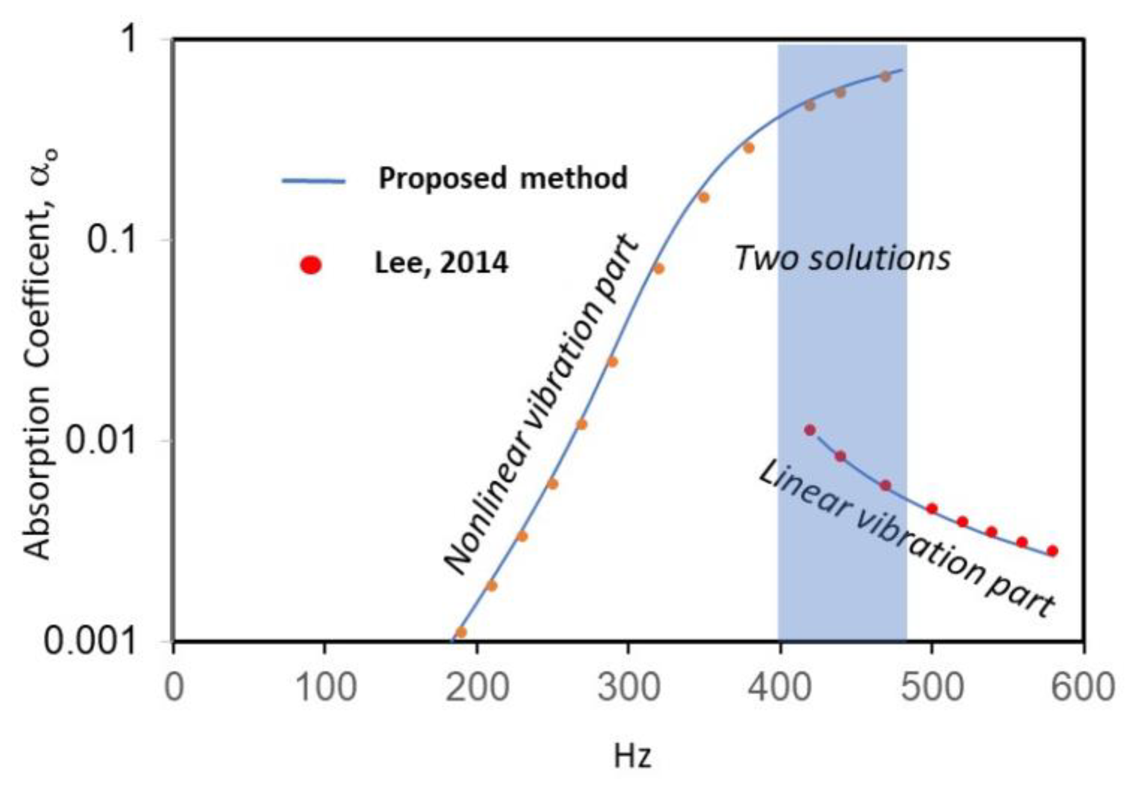
  33. Lee, Y.Y. Analytic formulation for the sound absorption of a panel absorber under the effects of microperforation, air pumping, linear vibration and nonlinear vibration. Abstr. Appl. Anal. 2014, 906506. [Google Scholar] [CrossRef] [Green Version]
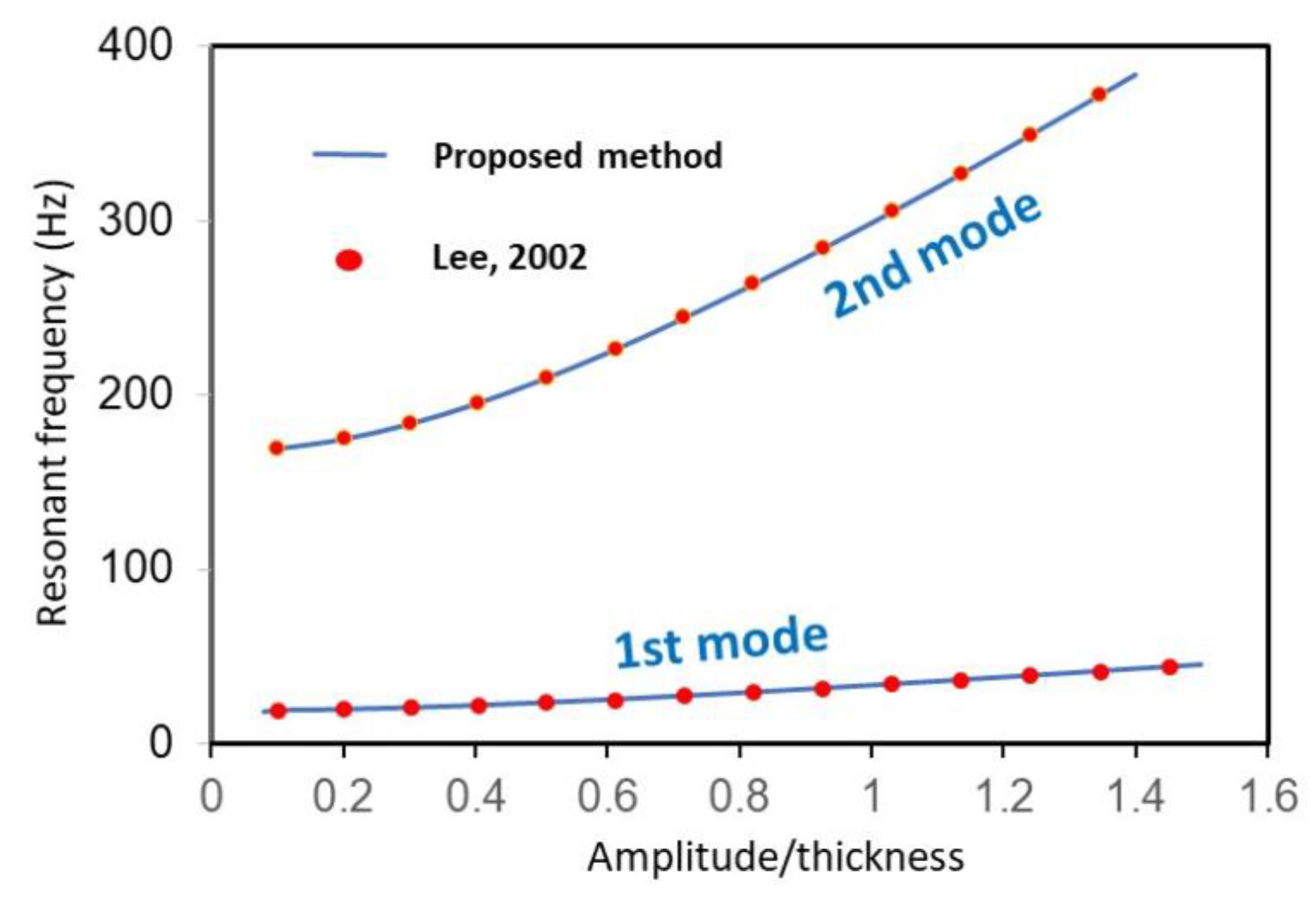
  34. Lee, Y.Y. Structural-acoustic coupling effect on the nonlinear natural frequency of a rectangular box with one flexible plate. Appl. Acoust. 2002, 63, 1157–1175. [Google Scholar] [CrossRef]
  35. Euler’s Method. Available online: https://lpsa.swarthmore.edu/NumInt/NumIntFirst.html (accessed on 1 May 2023).
Figure 1. Nonlinear curved perforated panel absorber.
Mathematics 11 03178 g001
Figure 2. Comparison between the absorption curves obtained from the proposed method and Lee, 2014 [33] for the nonlinear vibration case (h = 2 mm, a = 0.12 m, b = 0.1 m, ξ = 0.01, w o = 0   mm , κ = 30, no perforation effect).
Mathematics 11 03178 g002
Figure 3. Comparison between the resonant frequency curves obtained from the proposed method and Lee. 2002 [34] for the nonlinear vibration case (h = 2 mm, a = 0.4 m, b = 0.5 m, w o = 0   mm , no perforation effect).
Mathematics 11 03178 g003
Figure 4. Absorption curves for the nonlinear vibration case (h = 2 mm, a = 0.12 m, b = 0.1 m, ξ = 0.01, w o = 0   mm , κ = 30, d = 0.6 mm, σ = 0.11, D = 0.2 m).
Mathematics 11 03178 g004
Figure 5. Absorption curves for the chaotic vibration case (h = 2 mm, a = 0.4 m, b = 0.3 m, ξ = 0.01, w o = 10   mm , κ = 100, ω = 100 Hz, d = 0.6 mm, σ = 0.11, D = 0.2 m).
Mathematics 11 03178 g005
Figure 6. Time history for the chaotic vibration case (h = 2 mm, a = 0.4 m, b = 0.3 m, ξ = 0.01, w o = 10   mm , κ = 100, ω = 100 Hz, d = 0.6 mm, σ = 0.11, D = 0.2 m).
Mathematics 11 03178 g006
Figure 7. Phase plot for the chaotic vibration case (h = 2 mm, a = 0.4 m, b = 0.3 m, ξ = 0.01, w o = 10   mm , κ = 100, ω = 100 Hz, d = 0.6 mm, σ = 0.11, D = 0.2 m).
Mathematics 11 03178 g007
Figure 8. Time history for the chaotic vibration case (h = 2 mm, a = 0.4 m, b = 0.3 m, ξ = 0.01, w o = 10   mm , κ = 100, ω = 300 Hz, d = 0.6 mm, σ = 0.11, D = 0.2 m).
Mathematics 11 03178 g008
Figure 9. Phase plot for the chaotic vibration case (h = 2 mm, a = 0.4 m, b = 0.3 m, ξ = 0.01, w o = 10   mm , κ = 100, ω = 300 Hz, d = 0.6 mm, σ = 0.11, D = 0.2 m).
Mathematics 11 03178 g009
Figure 10. Time history for the chaotic vibration case (h = 2 mm, a = 0.4 m, b = 0.3 m, ξ = 0.01, w o = 10   mm , κ = 100, ω = 500 Hz, d = 0.6 mm, σ = 0.11, D = 0.2 m).
Mathematics 11 03178 g010
Figure 11. Phase plot for the chaotic vibration case (h = 2 mm, a = 0.4 m, b = 0.3 m, ξ = 0.01, w o = 10   mm , κ = 100, ω = 500 Hz, d = 0.6 mm, σ = 0.11, D = 0.2 m).
Mathematics 11 03178 g011
Figure 12. Absorption curves for the highly nonlinear and quasi-chaotic vibration cases (h = 2 mm, a = 0.4 m, b = 0.3 m, ξ = 0.1, w o = 10   mm , κ = 100, d = 0.6 mm, σ = 0.11, D = 0.2 m).
Mathematics 11 03178 g012
Figure 13. Time history for the highly nonlinear vibration case (h = 2 mm, a = 0.4 m, b = 0.3 m, ξ = 0.1, w o = 10   mm , κ = 100, ω = 100 Hz, d = 0.6 mm, σ = 0.11, D = 0.2 m).
Mathematics 11 03178 g013
Figure 14. Phase plot for the highly nonlinear vibration case (h = 2 mm, a = 0.4 m, b = 0.3 m, ξ = 0.1, w o = 10   mm , κ = 100, ω = 100 Hz, d = 0.6 mm, σ = 0.11, D = 0.2 m).
Mathematics 11 03178 g014
Figure 15. Time history for the quasi-chaotic vibration case (h = 2 mm, a = 0.4 m, b = 0.3 m, ξ = 0.1, w o = 10   mm , κ = 300, ω = 300 Hz, d = 0.6 mm, σ = 0.11, D = 0.2 m).
Mathematics 11 03178 g015
Figure 16. Phase plot for the quasi-chaotic vibration case (h = 2 mm, a = 0.4 m, b = 0.3 m, ξ = 0.1, w o = 10   mm , κ = 300, ω = 300 Hz, d = 0.6 mm, σ = 0.11, D = 0.2 m).
Mathematics 11 03178 g016
Figure 17. Time history for the highly nonlinear vibration case (h = 2 mm, a = 0.4 m, b = 0.3 m, ξ = 0.1, w o = 10   mm , κ = 100, ω = 500 Hz, d = 0.6 mm, σ = 0.11, D = 0.2 m).
Mathematics 11 03178 g017
Figure 18. Phase plot for the highly nonlinear vibration case (h = 2 mm, a = 0.4 m, b = 0.3 m, ξ = 0.1, w o = 10   mm , κ = 100, ω = 500 Hz, d = 0.6 mm, σ = 0.11, D = 0.2 m).
Mathematics 11 03178 g018
Table 1. Absorption convergence for various excitation frequencies, magnitudes, damping ratios and the number of modes (panel thickness h = 2 mm, panel length a = 0.4 m, panel width b = 0.3 m, hole diameter d = 0.6 mm, hole ratio σ = 0.11, cavity depth D = 0.2 m, ω = excitation frequency, w o = initial   center   deflection , k = excitation parameter, ξ = damping ratio).
ω = 100 Hz,
w o = 0   m m
k = 1, x = 0.01
ω = 300 Hz,
w o = 10   m m
k = 100, x = 0.04
ω = 300 Hz,
w o = 10   m m
k = 50, x = 0.01
ω = 300 Hz,
w o = 10   m m
k = 50, x = 0.04
1 mode99.22%94.47%94.14%99.33%
2 modes99.22%99.86%97.90%102.48%
3 modes100.00%100.00%99.25%100.00%
4 modes100.00%100.00%100.00%100.00%
Disclaimer/Publisher’s Note: The statements, opinions and data contained in all publications are solely those of the individual author(s) and contributor(s) and not of MDPI and/or the editor(s). MDPI and/or the editor(s) disclaim responsibility for any injury to people or property resulting from any ideas, methods, instructions or products referred to in the content.

