A Novel Finger Vein Verification Framework Based on Siamese Network and Gabor Residual Block

Abstract

The evolution of deep learning has promoted the performance of finger vein verification systems, but also brings some new issues to be resolved, including high computational burden, massive training sample demand, as well as the adaptability and generalization to various image acquisition equipment, etc. In this paper, we propose a novel and lightweight network architecture for finger vein verification, which was constructed based on a Siamese framework and embedded with a pair of eight-layer tiny ResNets as the backbone branch network. Therefore, it can maintain good verification accuracy under the circumstance of a small-scale training set. Moreover, to further reduce the number of parameters, Gabor orientation filters (GoFs ) were introduced to modulate the conventional convolutional kernels, so that fewer convolutional kernels were required in the subsequent Gabor modulation, and multi-scale and orientation-insensitive kernels can be obtained simultaneously. The proposed Siamese network framework (Siamese Gabor residual network (SGRN)) embeds two parameter-sharing Gabor residual subnetworks (GRNs) for contrastive learning; the inputs are paired image samples (a reference image with a positive/negative image), and the outputs are the probabilities for accepting or rejecting. The subject-independent experiments were performed on two benchmark finger vein datasets, and the experimental results revealed that the proposed SGRN model can enhance inter-class discrepancy and intra-class similarity. Compared with some existing deep network models that have been applied to finger vein verification, our proposed SGRN achieved an ACC of $99.74\%$ and an EER of $0.50\%$ on the FV-USM dataset and an ACC of $99.55\%$ and an EER of $0.52\%$ on the MMCBNU_6000 dataset. In addition, the SGRN has smaller model parameters with only 0.21 $\times {10}^6$ Params and 1.92 $\times {10}^6$ FLOPs, outperforming some state-of-the-art FV verification models; therefore, it better facilitates the application of real-time finger vein verification.

1. Introduction

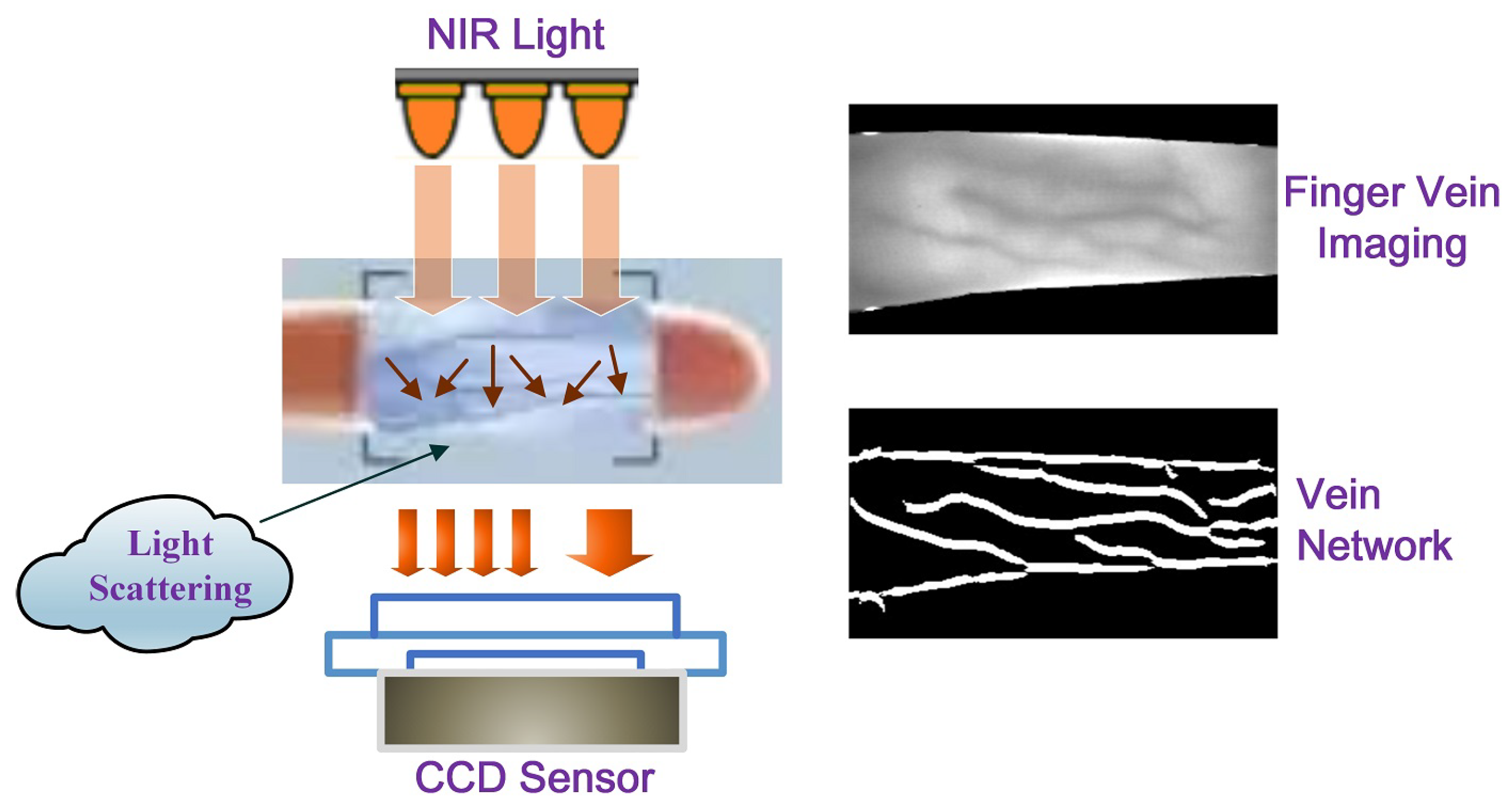
Currently, traditional technologies of personal identity authentication (e.g., tokens, cards, PINs) have been gradually replaced by some more-advanced biometrics technologies [1], including faces, retinas, irises, fingerprints, veins, etc. Among these, the finger vein (FV) trait [2], due to its unique advantages of high security, the living requirement, being non-contact, and not easily being injured or counterfeited, has drawn extensive attention after it appeared. Different from some visual imaging traits such as faces and fingerprints, the main veins in the fingers tend to be longitudinally distributed in the subcutaneous regions. Generally, FV imaging can be performed by using near-infrared (NIR) light in the particular wavelength range of (700∼1000 nm). When the NIR light irradiates the skin and enters the subcutaneous tissues, light scattering occurs, and plenty of light energy is absorbed by the deoxyhemoglobin in the veins’ blood, which makes the veins appear as dark shadows during imaging, while other non-vein areas show higher brightness. As a result, the acquired FV images generally present a crisscross pattern, as shown in Figure 1.

When the FV trait is used for personal identity verification, it should not be regarded as a conventional pattern-classification problem, due to the fact that the number of categories is huge, while the number of samples per category is small, and it occurs in a subject-independent scenario with only a subset of categories known during the training phase. Moreover, because of the restrictions of the acquisition equipment and environment, the imaging area of the vein texture is small [3] and the information carried by the vein image is relatively weak. In this regard, how to extract more-robust and -discriminative FV features is particularly critical for an FV verification system [4].

In the early stages of research, some meticulously hand-crafted features were adopted by FV verification systems. One kind of method, namely “vein-level” [5], was devoted to characterizing the geometric and topological shapes of the vein network (such as point-shaped [6,7,8,9], line-shaped [10,11], curve-based [12,13,14], etc.). In addition, anatomical structures [15,16] and even vein pulsation patterns [17] were also introduced for feature representation. In order to minimize the impact of the background as much as possible, these methods should accurately strip out the veins from the whole image. However, owning to the unexpected low quality of the acquired FV image, it has always been a great challenge to screen out the vessels accurately, while either over-segmentation or under-segmentation is the actual situation [18]. The “vein-level” features depend on pure and accurate vein pattern extraction, while neglecting the spatial relationship between veins and their surrounding subcutaneous tissues. As claimed in [19], the optical characteristics such as absorption and scattering in those non-vein regions were also helpful for recognition. Following this research line, another kind of method, namely “image-level” [5], aimed at extracting features from the whole image, while not distinguishing vein and non-vein regions. Among these, some local-pattern-based image features (e.g., local line binary pattern (LLBP) [20,21], local directional code (LDC) [22], discriminative binary code (DBC) [23]) have been widely adopted. Accompanying this, subspace-learning-based global image feature approaches, such as PCA [24,25] and LDA [26], have also been applied. Furthermore, such local and global features have been integrated to construct more-compact and -discriminative FV features [27].

The design of the aforementioned hand-crafted features usually depends on expert knowledge and lacks generalization over various FV imaging scenarios. Admittedly, these methods always rely on many preprocessing strategies to solve problems such as finger position bias, uneven illumination, etc. Relatively speaking, learning-based methods can provide more-adaptive feature representation, especially for the convolutional neural network (CNN)-based deep learning (DL) methods, which adopt a multi-layer nonlinear learning process to capture high-level abstract features from images [28,29,30]. Currently, CNNs equipped with various topological structures have been migrated to FV biometrics and have obtained commendable success. Among these, a deep CNN, namely “DeepVein” [31], was constructed based on the classic VGG-Net [32]. In [33], AlexNet was directly transferred to FV identification. In [34], convolutional kernels with smooth line shapes were especially picked out from the first layer of AlexNet and used to construct a local descriptor, namely the “Competitive Order”. In [35], multimodal biometrics, including finger veins and finger shape, were extracted from ResNet [36], respectively, and then fused for individual identity authentication. In [37], two FV images were synthesized as the input to DenseNet [38], while in [39], vein shape feature maps and texture feature maps were input into DenseNet in sequence and then fused for FV recognition. It must be conceded that DenseNet, due to its dense connection mechanism, generally has higher training complexity than AlexNet, VGG-Net, and ResNet [40].

The above classic DL models mostly adopt a data-driven feature-learning process, and their learning ability primarily relies on the quantity and quality of available image samples [41]. However, this is unrealistic in the FV community as most publicly available FV datasets are small-scale [42]. To address this issue, some fine-tuning strategies [43] and data augmentation technologies have been introduced to make up for the samples shortage to some extent. On the other hand, since vein images generally contain some low-level and mid-level features (mainly textures and shape structures), wider networks rather than deeper ones are preferred to learn a variety of relatively shallow semantic representations. In this regard, model distillation and lightweight models are also exploited for FV identity discrimination. In [44], a lightweight DL framework with two channels was exploited and verified on a subject-dependent FV dataset. In [45], a lightweight network with three convolution and pooling blocks, as well as two fully connected layers was constructed, and a joint function of the center loss and Softmax loss was designed to pursue highly discriminative features. In [46], a lightweight network, which consisted of a stem block and a stage block, was built for FV recognition and matching; the stem block adopted two pathways to extract multi-scale features, respectively, and then, the extracted two-way features were fused and input into the stage block for more-refined processing. In [47], a pre-trained Xception network was introduced for FV classification; due to depthwise separable convolution, the Xception network obtained a lighter architecture; meanwhile, the residual skip connection further widened the network and accelerated the convergence. These lightweight deep networks greatly lessen the training cost while ensuring accuracy, thus being more suitable for real-time applications of the FV trait.

Recently, some more-powerful network architectures have been used for FV recognition tasks, such as the capsule network [48], the convolutional autoencoder [49], the fully convolutional network [50], the generative adversarial network [51], the long short-term memory network [52], the joint attention network [53], the Transformer network [54], the Siamese network [55], etc. Among these, a Siamese framework, which is equipped with two ResNet-50s [36] as the backbone subnetwork, was introduced for FV verification [55]. Compared with some DL networks, which are inclined to learn better feature representation, the Siamese networks tend to learn how to discriminate between different input pairs by using a well-designed contrastive loss function. Therefore, they are more suitable for FV verification tasks, that is they better distinguish between genuine FVs and imposter FVs, rather than obtaining more-accurate semantic expressions. However, although the aforementioned network models have shown a strong feature-learning ability, they have the disadvantages of a complex model structure and an expensive training cost (

Table 1. A brief summary of the advantages and disadvantages of existing finger vein verification methods or models.

	Category	Methods/Models	Advantages	Disadvantages
Hand-Crafted	Vein-Level	Point [7,8], Line [10,11]	Pure	Lack Generalization
		Curvature [12,13,14]	Vein Pattern
		Anatomy [15,16]	Representation
		Vein Pulsation [17]
	Image-Level	LLBP [20,21]	Do Not Distinguish
		LDC [22]	Vein and Non-Vein
		DBC [23]	Regions
Learning-Based	Classic Models	DeepVein [31]
		AlexNet [33,34]	Capture High-Level	Complex Network Structures,
		ResNet [36]	Abstract Features	Massive Sample Requirement
		DenseNet [39]
	Powerful Models	Capsule [48], CAE [49], FCN [50]
		GAN [51], LSTM [52]	Stronger
		Joint Attention Network [53]	Feature	More Complex Network Structures
		Transformer Network [54]	Representations
		Siamese Network [55]
	Lightweight Models	Two-Stream CNN [44]	Simper Network
		Light CNN [45,46]	Structures, Lower	Feature Representation Is Weak
		Xception [47]	Computation Cost

).

As noted above, hand-crafted FV features lack generalization ability, while some classic and powerful DL models often have complex network structures and rely on massive labeled samples for training. Considering that the realistic finger vein verification scenario often has a limited number of labeled samples, we were committed to constructing a lightweight network model and specifically addressed the following problems: First, since the ultimate goal of the FV verification task was to distinguish whether a pair of input samples belongs to the same finger or not, so as to make a decision to accept or reject, our proposed model focused on improving the discrimination ability, rather than just the representation ability of the features. Second, since an imbalance problem existed due to the small number of in-class samples and the large number of categories, we tried to construct a Siamese contrast learning framework to adapt to such an imbalance and mitigate overfitting issues. Lastly, since FV verification is essentially a subject-independent classification scenario, with many unknown categories of samples appearing during the testing phase, we introduced Gabor filters to improve the robustness of the conventional convolutional kernel and its ability to characterize multiple scales and multiple orientations.

In a nutshell, we propose a novel end-to-end Siamese network framework with two parameter-sharing and Gabor-modulated tiny ResNet branches (dubbed the Siamese Gabor residual network (SGRN)). The main innovative contribution of our work is three-fold:

• First and foremost, we introduced a Gabor-modulated convolutional kernel (dubbed GRNs) to replace the conventional convolutional kernels in two subnetworks, which aimed to model both rotation invariance and the more complicated transformation invariance, thus enhancing the deep feature representation with steerable orientation and scale capacities.
• Second, in the proposed SGRN model, two parameter-sharing branch networks were embedded for contrastive learning. By incorporating tiny ResNet structures and Gabor-modulated convolutions, the SGRN can be regarded as a lightweight discriminant network, which is suitable for the practical application scenarios of FV traits.
• Third, exhaustive experiments were carried out on two benchmark FV datasets, and the experimental results revealed the effectiveness of our proposed SGRN. Besides, by using Gabor orientation filters (GoFs) to modulate the convolutional kernels, we observed that fewer convolutional kernels were required for the subsequent Gabor modulation stage, thus leading to fewer model parameters and a more-robust feature representation ability.

The remainder of this paper is organized as follows. Section 2 provides a brief review of the related works, including the basic procedure of FV verification, the Siamese network framework, and the Gabor convolutional kernel. Section 3 details the proposed SGRN architecture and corresponding training strategy. Section 4 provides the experimental results obtained by using two benchmark FV datasets. Section 5 presents the discussion of this research work. Section 6 concludes the paper with some remarks and hints at plausible future research lines.

2. Related Works

In this section, we first provide a brief overview of the basic procedure of FV verification, then we will give a brief explanation about two key components, the Siamese network framework and Gabor convolutional kernel.

2.1. Basic Procedure of Finger Vein Verification

In general, the processing flow of an FV verification system consists of four tasks: image capturing, preprocessing, feature extraction, and feature matching, as shown in Figure 2. Among these, the stages of image preprocessing and feature extraction are the most-critical ones; some preprocessing strategies, such as ROI localization and contrast enhancement, have a significant impact on the subsequent feature extraction. In the meantime, a powerful feature representation ability is key to precise matching.

As stated earlier, deep CNNs have shown the capability to learn unprecedentedly efficient image features. However, most of the existing DL models regard feature extraction and feature matching as two separate stages, thus lacking a comprehensive consideration of feature learning from the perspective of discriminant matching. Instead, the Siamese network combines both of these through contrastive learning, so that the learned features can better serve the final matching purposes.

2.2. Siamese Network Framework

A Siamese network is usually equipped with a pair of subnetworks, as shown in Figure 3. For a pair of input samples, their feature vectors are learned by the corresponding subnetworks and then given to the contrastive loss function for similarity measurement. Generally, the contrastive loss function can be defined by Equation (1).

$$\begin{array}{cc}\hfill \mathrm{Loss}(X_1,X_2)& =(1-\gamma )\frac{1}{2}{\left(D_w\right)}^2+\left(\gamma \right)\frac{1}{2}{\{max(0,m-D_w)\}}^2,\hfill \end{array}$$

(1)

where $D_w$ is the similarity distance metric, $\gamma$ is an indicator of whether the prediction is from the same finger class, $\gamma$ equals 0, otherwise, $\gamma$ equals 1, and m is a positive margin value, which is used to protect the loss function from being corrupted when the distance metric of different sample pairs exceeds this margin value.

2.3. Gabor Convolutional Kernel

The Gabor convolutional kernel represents a combination of classic computer vision and deep neural networks; similar works have proven it to be successful [56]. According to their combination strategies, existing methods can be divided into three categories: The first category regards the Gabor filter as a kind of preprocessing, which means the inputs of the CNNs are Gabor-filtered images. Furthermore, in [57], convolutional kernels in the first two layers of the CNN were replaced by Gabor filters with fixed parameters. In this case, although the parameters of the trainable network were reduced, it still lacked a deep combination of the Gabor filters’ representation ability and the CNN’s learning ability. The second category completely replaces the convolutional kernels with Gabor filters and optimizes the parameters of the Gabor filters. Among these, in [58], only the first layer was replaced by the Gabor filters, while the remaining layers remained unchanged. In [59], a parameterized Gabor convolutional layer was used to replace a few early convolutional layers in the CNNs, and it obtained a consistent boost in accuracy, robustness, as well as highly generalized test performance. However, due to the computational complexity of the Gabor convolution operation and the corresponding parameter optimization algorithm, its popularization has been restricted. The third category adopts Gabor filters to modulate the learnable convolutional kernels [60]. Compared with the above two categories, such a method allows the network to capture more robust features with regard to orientation and scale changes, while not bringing additional computational burden.

3. Proposed Method

This section provides a detailed explanation of each part of the SGRN architecture. Firstly, the Gabor orientation filter is introduced to replace the conventional convolutional kernel. Secondly, Gabor-modulated convolutional kernels are integrated into a tiny ResNet, which stood as the backbone branch networks of our SGRN model. Finally, the whole structure of the SGRN is presented.

3.1. Gabor Orientation Filter

Considering that vein images mainly rely on texture and structure information to discriminate individuals, we adopted a Gabor-modulated orientation filter to encode the directionality and multi-scale characteristics. Concretely, suppose ${\mathcal{C}}_i$ is a learned 2D convolutional kernel in the i-th layer of the CNN, which generally has a size of $k\times k$ and $k^2$ parameters, and $\mathcal{G}(\mu ,\nu )$ is a Gabor filter with orientation $\mu$ and frequency $\nu$. Thus, the Gabor-modulated convolutional kernel can be generated by using Equation (2):

$${\mathcal{C}}_{i,\mu }^{\nu }={\mathcal{C}}_i\otimes \mathcal{G}(\mu ,\nu ),$$

(2)

where ${\mathcal{C}}_{i,\mu }^{\nu }$ denotes the modulated convolutional kernel and ⊗ is an elementwise filtering operation on ${\mathcal{C}}_i$ by using Gabor filter $\mathcal{G}(\mu ,\nu )$. When providing U orientation parameters for a given frequency $\nu$, there will be a Gabor filter bank of $\left\{\mathcal{G}\right(1,\nu ),\dots ,\mathcal{G}(U,\nu \left)\right\}$. In this case, the steerable filter group created by manipulating the above U Gabor filters on the learned convolutional kernel ${\mathcal{C}}_i$ can be expressed by Equation (3).

$${\mathcal{C}}_i^{\nu }=({\mathcal{C}}_{i,1}^{\nu },\dots ,{\mathcal{C}}_{i,U}^{\nu }),$$

(3)

where ${\mathcal{C}}_i^{\nu }$ is called a convolutional Gabor orientation filter (GoF). Furthermore, given a Gabor filter bank with U orientations and V scales, we can generate V groups of GoFs, and each group of GoFs contains U orientation filters at a specific scale.

In each Gabor residual subnetwork of the SGRN model, with the advance of the convolutional layers, the GoFs with increasing scales will be adopted synchronously; in other words, the orientation information is encoded into each learned convolutional kernel, and the scale information is embedded into different convolutional layers simultaneously.

3.2. Gabor Residual Network

The proposed Siamese network framework embeds a pair of lightweight discriminant branch networks for contrastive learning. Specifically, we introduced a tiny ResNet with fewer than 8 convolutional layers [61]. As shown in Figure 4a, this tiny ResNet contains 7 convolutional unit blocks, followed by one pooling layer and one fully connected layer.

In a routine DL network, the processing pipeline has one path and feature learning performs sequentially from one layer to the next layer. However, ResNet breaks through this limitation and introduces a simple identity skip connection to allow shortcuts to be formed between different layers. This strategy can be viewed as a collection of multiple paths instead of a single-path deep network [36]. Indeed, unlike some common image classification scenarios, FV images mainly depend on some low-level and mid-level semantic features to distinguish individuals. Here, low-level semantic features generally contain edges, textures, shapes, etc., and mid-level semantic features generally contain some attribute features, such as the vein structure and vein distribution. Therefore, the designed backbone network architecture should maintain a broader structure rather than continuously deepening it. In this regard, the adopted tiny ResNet provides a wide and shallow network structure to learn a variety of relatively low-level structural features. Thus, on the premise of effective verification accuracy, the model complexity and training pressure are significantly reduced and more conducive to the deployment and application of an FV verification system.

Furthermore, in order to enhance the ability to extract texture and structure information from the FV images, as well as reduce the redundancy of the convolutional kernels, we introduced the GoFs to replace the standard convolutional kernels of each convolutional layer in the tiny ResNet and form the Gabor residual networks (GRNs), as shown in Figure 4b.

The motivations for adopting the GoFs were as follows: Given no prior knowledge, conventional CNNs have to use as many standard convolutional kernels as possible to cover more comprehensive image feature representations, which results in a large number of redundant convolutional kernels to be learned. In this regard, some prior knowledge can be injected into those standard convolutional kernels, so as to use fewer, but more-purposeful convolutional kernels to learn discriminant features. Among these, the Gabor filters have an inherent joint time–frequency resolution, which can extract low-level and mid-level features. When combining Gabor filters with standard convolutional kernels, not only shift-invariance can be injected into the network, but also rotation and scale invariance are also reinforced.

Through these adjustments, the output feature maps in each convolutional layer of the GRNs are calculated by using Equation (4).

$${\widehat{\mathcal{F}}}_{i,\mu }=\sum _{n=1}^N{\mathcal{F}}^{\left(n\right)}\otimes {\mathcal{C}}_{i,\mu }^{\nu },$$

(4)

where ${\mathcal{F}}^{\left(n\right)}$ refers to the n-th channel of the input feature maps $\mathcal{F}$ and ${\widehat{\mathcal{F}}}_{i,\mu }$ denotes the $\mu$ orientation response of ${\widehat{\mathcal{F}}}_i$. As a result, these Gabor-modulated convolutional kernels gain the capability to encode direction and scale. For convenience, we present the detailed network configurations of the GRN in

Table 2. Configurations of each GRN in the proposed SGRN framework. Among these, “GC” denotes the Gabor orientation filter, “AP” denotes average pooling, and “FC” denotes fully connected.

♯	Layer Type	Number of Kernels/	Gabor Params	Output Size
		Size/Stride	$\mathit{\mu }$,$\mathit{\nu }$
0	Input	–	–	$32\times 32\times 1$
1	GC	4/$7\times 7$/1	$\mu$ = 4, $\nu$ = 1	$32\times 32\times 16$
2	GC	4/$3\times 3$/1	$\mu$ = 4, $\nu$ = 2	$32\times 32\times 16$
3	GC	4/$3\times 3$/1	$\mu$ = 4, $\nu$ = 2	$32\times 32\times 16$
4	GC	8/$3\times 3$/1	$\mu$ = 4, $\nu$ = 3	$32\times 32\times 32$
5	GC	8/$3\times 3$/2	$\mu$ = 4, $\nu$ = 3	$16\times 16\times 32$
6	GC	16/$3\times 3$/1	$\mu$ = 4, $\nu$ = 4	$16\times 16\times 64$
7	GC	16/$3\times 3$/2	$\mu$ = 4, $\nu$ = 4	$8\times 8\times 64$
8	AP	stride = 2	–	$4\times 4\times 64$
9	FC	–	–	$200\times 1$

.

As can be observed from Table 2, the first convolutional layer of the GRN adopted 4 standard convolutional kernels and a Gabor modulating filter bank under 4 orientations ($[{45}^{\circ },{90}^{\circ },{135}^{\circ },{180}^{\circ }]$) and scale $\nu =1$, thus forming a total of $4\times 4=16$ modulated convolutional kernels. As a result, the output of the first convolutional layer is 16 feature maps for each input image. Then, there are three consecutive residual blocks; each contains two convolutional groups, which means, a convolutional layer, a batch normalization, and a ReLU nonlinear layer form a convolutional group. For each residual block, the Gabor filters adopted a changing scale from $\nu =1$ to 4, representing the scale from coarse to fine. Thus, the identity skip connection will fuse the output of the two neighborhood residual blocks. It should be noted that, in the second and third residual blocks, we set stride = 1 and stride = 2 for two successive convolutional layers, respectively. In this case, the downsampling of the feature maps will occur in each residual block and bring about inconsistent sizes of the feature maps at both ends of the residual connection, so we adopted a $1\times 1$ convolution operation to align the sizes of the feature maps. After this, the output feature maps of the seventh convolutional layer are further downsampled by an average pooling layer, as well as flattened to a one-dimensional vector. Finally, the feature vector is input into a fully connected layer to form the output feature representation of each branch of the GRN.

3.3. Framework of Siamese Gabor Residual Network

The overall architecture of the SGRN is shown in Figure 5; it is known as an end-to-end metric-learning network, containing two parameter-sharing branch subnetworks; in this case, the GRN acts as the branch network, and because of the weight sharing, the same convolutional kernels are used in each GRN and trained from scratch.

The inputs of the SGRN are a couple of sample images; a reference image with a positive image is called the same-class sample pair, while a reference image with a negative image is called a different-class sample pair. First, these two sample images are fed into the two subnetworks of the SGRN, respectively, so as to learn their corresponding latent encoding feature representation. Then, two encoding feature vectors are concatenated and used to produce the probabilities of whether they are from the same finger class or not, meaning accepting or rejecting. Here, we adopted a specially designed concatenation strategy. Specifically, supposing the output of each GRN branch is an n-dimensional vector (in our GRNs, n was equal to 200), the concatenation of these two n-dimensional vectors is performed by using Equation (5).

$${\mathbf{v}}_{union}=[{\mathbf{v}}_a,{\mathbf{v}}_b,{({\mathbf{v}}_a-{\mathbf{v}}_b)}^2,{\mathbf{v}}_a\odot {\mathbf{v}}_b],$$

(5)

where ${\mathbf{v}}_a$ and ${\mathbf{v}}_b$ are the output feature vectors corresponding to each couple of FV images, ${({\mathbf{v}}_a-{\mathbf{v}}_b)}^2$ denotes the square of their differences, and ${\mathbf{v}}_a\odot {\mathbf{v}}_b$ denotes the Hadamard product of two vectors. As a result, the concatenated vector is four times the length of ${\mathbf{v}}_a$. Subsequently, the concatenated vector is fed into a fully connected layer with two hidden units to output the class scores, and these scores are used to train the SGRN model with the Softmax cross-entropy loss.

In the SGRN framework, the Softmax classifier is used to predict the probability of matching or not. In this manner, the model can simultaneously learn the feature representation and distance function with the best class separation. In addition, even if the raw samples are not sufficient, we can use the combination of these limited samples to generate a large number of training sample pairs to facilitate model learning; the SGRN model will traverse all the sample pairs with gradient descent and constantly update the network parameters until the loss function becomes stable or reaches the maximum number of iterations.

After the SGRN model has been well trained, it will be used to predict the matching result of two input testing images, and the ultimate predicted output will be derived from the maximum of the two confidence scores.

In summary, compared with some existing network models, our proposed SGRN model has some special designs: First, corresponding to the 18-layer ResNet backbone subnetworks in the Siamese CNN [55], we trimmed them to an extreme 8-layer ResNet backbone to further simplify the network structure. Then, we introduced Gabor filters to modulate the standard convolutional kernels and performed convolution operations with the modulated GoFs. In this case, by using relatively few standard convolutional kernels in each layer, it was possible to allow the network to capture robust features with regard to scale and orientation changes. Furthermore, because the Gabor modulation process does not bring any additional learning parameters, the training overhead of the network was not increased much. Finally, we designed a special concatenation strategy for the output features of two subnetworks of the GRN, which greatly improved the discrimination ability of the concatenated features and subsequent verification accuracy. Through the above series of unique designs, the final network model showed better performance under various evaluation metrics.

4. Experimental Results and Discussion

In this section, to ascertain the effectiveness of our SGRN model, we carried out comprehensive experimental analysis on two benchmark FV datasets, “MMCBNU_6000” [62] and “FV-USM” [63]. First, Section 4.1 provides a brief description of the adopted FV datasets. Second, Section 4.2 presents the relevant parameter settings, as well as the training and testing procedures of the proposed SGRN model. In Section 4.3, the adopted evaluation metrics are reported. Next, in Section 4.4, the sensitivity of some key parameters is quantitatively assessed. After, in Section 4.5, aiming for the key structural design of the SGRN model, we carry out ablation study on the GRN branch network and contrastive-learning-based loss function, respectively. Finally, a few mainstream CNN-based FV verification methods are compared with our SGRN in Section 4.6.

4.1. Finger Vein Datasets

In our experiments, two benchmark FV datasets, MMCBNU_6000 and FV-USM, were chosen to assess the performance of the SGRN model; both datasets provide tailored ROI images, and we directly used these ROI images for the analysis in the following experiments.

The “FV-USM” [63] dataset was published by the University of Sains Malaysia. It consists of 5904 jpg images with a size of $640\times 480$, all images are taken from 123 subjects with four fingers per subject. Considering that every finger is a distinct class, there is a total of 492 classes. The images of “FV-USM” were acquired in two different sessions with six images per finger in every session. The corresponding ROI images have a size of $50\times 150$.

The “MMCBNU_6000” database [62] was collected by 100 volunteers from 20 countries and published 600 classes with 10 images for each class, thus forming 6000 sample images. The original sample images are all grey-scale images, with a size of $640\times 480$. The corresponding ROI images have a size of $128\times 60$.

More detailed descriptions of the above two FV datasets are shown in

Table 3. Details of the two finger vein datasets.

Dataset	Subjects	Fingers	No. of Fingers	Images per Finger	Session	Total Images	Orientation of Fingertip
FV-USM  [63]	123	middle index (left, right)	492	12	2	5904	down
MMCBNU_6000 [62]	100	middle ring (left, right)	600	10	1	6000	right

. It is worth emphasizing that both FV datasets are small-scale sample sizes, that is the number of samples provided by each category is very small, e.g., 6 samples per category in “FV-USM” (we chose only one set of session data for the experiment) and 10 samples per category in “MMCBNU_6000”, while the number of corresponding categories reached 492 and 600. Therefore, the experiments carried out on the above two FV datasets can be regarded as being performed in a small-scale sample scenario. Moreover, some acquired sample images are shown in Figure 6; it can be observed that the orientation of the fingertip is downward in the “FV-USM” dataset, while the orientation of the fingertip is toward the right in the “MMCBNU_6000” dataset. In this case, many methods have to adjust the acquired images to a uniform orientation beforehand, thus bringing additional preprocessing overhead and affecting the generalization performance of the algorithm. Conversely, in our proposed SGRN model, the Gabor orientation filter was introduced to modulate the conventional convolution filter, thus showing insensitivity to the orientation of the fingers. As a result, instead of rotating the acquired sample images to maintain the uniform orientation, we directly used the original images with different orientations as the input of the SGRN model, which not only reduced the burden of preprocessing, but also improved the generalization ability of the algorithm.

4.2. Experimental Settings and Training/Testing Procedures

Generally, in an FV verification scenario, we can perform subject-independent or subject-dependent experiments. In the subject-dependent experiment, all available classes need to be used during training and testing. However, this is not a realistic situation, since we are unable to obtain all categories during the training process. In this regard, it is more suitable to perform the experiment in an subject-independent scenario, which means parts of the available classes are used for training, while the rest and even new classes are used for testing, so as to guarantee a disjoint relationship between the training and testing sets.

In the following experiments, we carried out a subject-independent configuration. Specifically, the above FV dataset was randomly divided into two disjoint parts, of which $90\%$ was used for training, while the remaining $10\%$ was used for testing, and a 10-fold cross-validation was conducted to report the experimental results. Specifically, for FV-USM, 50 classes were used for testing, with a total of 300 image samples, while 442 classes with a total of 2652 images were left for training. For MMCBNU_6000, there were 60 classes with a total of 600 images used for testing, while the remaining 540 classes with a total of 5400 images were used for training.

Considering that the input of the SGRN is a pair of sample images, we adopted the following strategies to generate positive and negative sample pairs, respectively. For a positive match pair, we traversed over all sample images from the same finger class and paired them up. Concretely, for FV-USM, since 442 classes were used to construct the sample pairs and each class had six images, we could build 15 positive match pairs for each class, thus forming a total of $15\times 442=6630$ positive match pairs. For MMCBNU_6000, 540 classes with 10 images per class were used to construct the sample pairs; we could build 45 positive match pairs for each class, thus forming a total of $45\times 540=\mathrm{24,300}$ positive match pairs. For the negative mismatch pairs, which were composed of images from different classes, we could obtain a huge number of negative sample pairs. In this case, if we used a 1:1 ratio, the total number of training pairs was too small to perform effective model training. However, if all available positive/negative sample pairs were used, the problem of a significant imbalance would arise. As a compromise, we chose one finger image, then paired it with randomly selected sample images in the other different finger classes as negative pairs and kept the ratio of positive and negative sample pairs at 1:5, thus forming a total of 39,780 training sample pairs in FV-USM and 145,800 training sample pairs in MMCBNU_6000. Note that the labels for the training sample pairs were set to 0 and 1, where 1 represents that the sample pair came from the same finger class, while 0 represents that the sample pair came from different finger classes. Following the same strategy, we also generated the corresponding test sample pairs, as detailed in

Table 4. Proportion details of each finger vein dataset.

Dataset	Train Class	Train Samples	Train Pairs	Test Class	Test Samples	Test Pairs
FV-USM	442	2652	39,780	50	300	4500
MMCBNU_6000	540	5400	145,800	60	600	16,200

.

The initial network weights in the convolutional layers of the GRN were set by using a normal distribution with 0 mean and a standard deviation of 0.01, and the biases were also initialized from a normal distribution, but with a mean of 0.5 and a standard deviation of 0.01. In the fully connected layers, the weights were drawn from a normal distribution with 0 mean and a standard deviation of 0.2, and the biases were initialized by adopting the same way as in the convolutional layers.

During the training procedure, the input of the SGRN was batches of sample pairs, where the sizes of the sample images were both $32\times 32$, and the batch size was set to be 50. The whole training process of the SGRN contained two steps: forward propagation and backpropagation. In the forward propagation procedure, each sample pair was fed into the two-branch GRN to learn their corresponding feature vectors. Then, the concatenation of the two feature vectors was performed, and this was fed into the subsequent fully connected layer to calculate the category probability. In the backpropagation procedure, the Softmax cross-entropy loss function was computed, and the Adam optimization method was adopted to update the network parameters, while the corresponding learning rate was set to $2\times {10}^{-5}$.

After the SGRN model was well-trained, it was used to predict the verification results of each test image pair. Given that the output of the Softmax classifier is a sample-to-class probability value, the final prediction result was derived from the maximum class confidence score. At this point, we did not need to find an appropriate threshold to help us ensure that the sample pairs were from the same finger class as in the common recognition scenario, which has always been a difficult task in and of itself. On the contrary, thanks to the contrastive learning mechanism adopted by the SGRN model, the output category contained only two choices, either belonging to the same finger class or coming from different classes.

4.3. Evaluation Metrics

In order to quantitatively evaluate the verification performance of the SGRN model, we adopted some typical metrics in the experiments:

• The false acceptance rate (FAR), which is the ratio of the number of accepted imposter claims divided by the number of verification attempts, as shown in Equation (6).

  $$\mathrm{FAR}=\frac{fa\_num}{ia\_num}\times 100\%,$$

  (6)

  where $\mathrm{fa}\_\mathrm{num}$ is the number of false accepted claims and $\mathrm{ia}\_\mathrm{num}$ is the number of impostor verification attempts.
• The false rejection rate (FRR), which is the ratio of the number of false rejections divided by the number of verification attempts. The related formula is shown in Equation (7), where $\mathrm{fr}\_\mathrm{num}$ is the number of false rejections and $\mathrm{gra}\_\mathrm{num}$ is the number of genuine verification attempts.

  $$\mathrm{FRR}=\frac{fr\_num}{gra\_num}\times 100\%,$$

  (7)
  Taking each finger as one class, if there are n finger classes and each finger class has m images, $\mathrm{gra}\_\mathrm{num}$ will be $n\times m\times (m-1)/2$, and $\mathrm{ia}\_\mathrm{num}$ will be $5\times n\times m\times (m-1)/2$ (to keep the ratio of positive and negative, sample pairs at 1:5). In this case, the FRR can be viewed as a metric to measure intra-class correlation; a lower FRR means better intra-class similarity. For the FAR, it can be viewed as a metric of inter-class distance; a lower FAR means better inter-class discrepancy.
• The equal error rate (EER) is defined as the ratio of trials in which the FAR is equal to the FRR; a lower EER exhibits better performance in the FV verification tasks.
• The verification accuracy (ACC), which is the ratio of the number of correct verifications divided by the number of total verifications, as shown in Equation (8), where $N_T$ represents the number of sample pairs correctly classified and N represents the total number of sample pairs.

  $$\mathrm{ACC}=\frac{N_T}{N}\times 100\%,$$

  (8)

Finally, we would like to emphasize that all experiments were conducted by using Python 3.8 with the PyTorch 1.8.0 framework, running on a desktop PC equipped with the configurations of an Intel Core i7 CPU (at 3.6 GHz), 32 GB of RAM, and an NVIDIA GeForce GTX 1080 Ti GPU.

4.4. Analysis of Parameters’ Sensitivity

In this section, we analyze the sensitivity of some key parameters in the SGRN model, including the orientation and scale parameters of the Gabor filters, as well as the dimensions of the output feature vectors of each GRN network. All experiments were performed on both FV datasets; when one parameter was assessed in our experiments, the other parameters were fixed and set to the same values reported in Table 2.

4.4.1. Orientation and Scale of Gabor Filters

In this experiment, we evaluated the influence of the Gabor filters under different orientation and scale parameters. As previously mentioned, our GRN branch network adopted parameters with an increasing scale with the advance of the convolutional layers, so as to guarantee the scale information was embedded into the different convolutional layers. Therefore, we first compared the increasing scales strategy with a fixed scale in each convolutional layer.

Table 5. ACC (%) and EER (%) obtained by using different orientations and scales on FV-USM dataset.

Scale		1	2	3	4	5	6	INC
Dir
4	ACC (%)	99.62	99.71	99.76	99.58	99.58	99.60	99.74
	EER (%)	0.98	0.42	0.44	0.91	0.64	0.89	0.50
8	ACC (%)	99.29	99.53	99.30	99.49	99.49	99.51	99.81
	EER (%)	1.36	1.01	0.90	1.25	1.13	1.17	0.56

Bold is used to highlight the best value.

and

Table 6. ACC (%) and EER (%) obtained by using different orientations and scales on MMCBNU_6000 dataset.

Scale		1	2	3	4	5	6	INC
Dir
4	ACC (%)	99.38	99.46	99.64	99.24	99.36	99.57	99.55
	EER (%)	0.90	0.85	0.68	1.16	0.75	0.81	0.52
8	ACC (%)	99.51	99.45	99.51	99.36	99.10	99.52	99.43
	EER (%)	0.68	0.85	0.74	0.88	1.16	0.75	0.75

Bold is used to highlight the best value.

present the results of the ACC and EER under different scale strategies on FV-USM and MMCBNU_6000, respectively.

From Table 5, the Columns 1 to 6 represent that all convolutional layers in the GRN adopted a fixed scale parameter $\nu$ (e.g., “1” denotes a fixed scale $\nu =1$ in all convolutional layers), while the last column “INC” denotes an increasing scale of $\nu$ in multiple consecutive convolutional layers. Concretely, the first convolutional layer was set to $\nu =1$, and then, the next three consecutive residual blocks were set to $\nu =2,3,4$, respectively.

Observed from the perspective of the orientation parameters, when the scale parameter $\nu$ was fixed, the ACC results in the 4 orientations were better than the corresponding results in the 8 orientations; especially for the scale $\nu <4$, the average difference of ACC was greater than $0.3\%$; however, when the scale $\nu$ changed incrementally, there was little difference between the ACC results of the 4 orientations and 8 orientations. A similar phenomenon also appeared in the EER results; no matter whether in a single scale or in a consecutively increasing scale, the EER results of the 4 orientations were better than those of the 8 orientations. On the surface, this seemed to undermine the usual belief that the more orientations covered, the stronger the representation ability. However, in actual finger vein images, the distribution of the veins shows remarkable directionality attributes. Therefore, the use of four orientations was sufficient to enhance such directionality attribute representation. Considering that too many orientation parameters such as 8 orientations may induce overly complex network processing, while too few orientation parameters were not able to extract enough informative features, it was preferable to use 4 orientations.

From the perspective of the scale parameters, we can observe that there existed a best fixed scale parameter; for the ACC results, the best fixed scale was $\nu =3$ in the case of 4 orientations and $\nu =2$ in the case of 8 orientations. For the EER results, the best fixed scale was $\nu =2$ in the case of 4 orientations and $\nu =3$ in the case of 8 orientations. Intuitively, although such a best fixed scale parameter was hard to determine, it reflected that different scale parameters were necessary for different network layers. By using an incremental scale setting, the highest ACC result was obtained with 8 orientations, and the third-lowest EER was obtained with 4 orientations. However, it should be admitted that determining the scale parameters of the optimal adaptation for each layer requires further exploration.

For the MMCBNU_6000 dataset, the 4-orientation results were slightly better than the 8-orientation results, especially in the case of incremental scales. When the orientation parameter $\mu =4$, the incremental scale setting obtained the third-highest ACC, $0.09\%$ lower than the best ACC value, and obtained the lowest EER. For the eight orientations, the incremental scales also obtained near-optimal ACC and EER results.

In a nutshell, the four-orientation parameters had better performance gains. In terms of scale issues, although the incremental scale setting was better, how to determine the optimal scale parameters is still unresolved and even affected by the orientation parameters. After a comprehensive consideration, we adopted a Gabor filter bank with four orientations of $[{45}^{\circ },{90}^{\circ },{135}^{\circ },{180}^{\circ }]$ and an incremental scale of $\nu$ from 1 to 4 in our experiments.

4.4.2. Output Dimension Size

As mentioned earlier, the output feature vectors of the two-branch network was concatenated by using Equation (5) and then fed into a fully connected layer for class scores’ prediction. Obviously, different concatenation strategies and the length of the feature vectors will have a significant impact on the accuracy and parameters of the model, so we conducted experiments to assess the ACC, EER, model parameters (“Params”), and floating point operations (FLOPs) regarding these two issues.

Table 7. ACCs (%), EERs (%), Params, and FLOPs obtained by using different concatenation strategies on FV-USM dataset.

	ACCs (%)	EERs (%)	Params	FLOPs
$[{\mathbf{v}}_a,{\mathbf{v}}_b]$	83.64	46.82	209,034	1,919,781
$[{\mathbf{v}}_a,{\mathbf{v}}_b,{({\mathbf{v}}_a-{\mathbf{v}}_b)}^2]$	99.62	0.65	209,434	1,920,181
$[{\mathbf{v}}_a,{\mathbf{v}}_b,{({\mathbf{v}}_a-{\mathbf{v}}_b)}^2,{\mathbf{v}}_a\odot {\mathbf{v}}_b]$	99.74	0.50	209,834	1,920,581

Bold is used to highlight the best value.

shows the results obtained by using different concatenation strategies on the FV-USM dataset. It can be observed that the best ACC and EER results came from a concatenation of all four terms, including each couple of feature vectors, the square of their differences, and the Hadamard product of two vectors, especially for the latter two terms, which played an important role in distinguishing the two feature vectors.

Table 8. ACCs (%), EERs (%), Params ($\times {10}^6$), and FLOPs ($\times {10}^6$) obtained by using different output dimensions on FV-USM dataset.

	ACCs (%)	EERs (%)	Params ($\times {10}^6$)	FLOPs ($\times {10}^6$)
$100\times 4$	99.45	1.00	0.11	1.71
$200\times 4$	99.74	0.50	0.21	1.92
$300\times 4$	99.52	0.79	0.31	2.13

Bold is used to highlight the best value.

shows the corresponding results obtained by using different output dimensions of the GRN on the FV-USM dataset. Here, $100\times 4$ means each output feature vector of the GRN was a 100-dimensional vector, and after concatenation with Equation (5), there would be a 400-dimensional vector for the subsequent fully connected layer.

Indeed, the greater the dimension of the output feature vector, the richer the information contained therein and the better the result was. It can be proven from Table 8 that 200 dimensions is better than 100 dimensions. However, the ratio of the input and output dimensions essentially reflected a low-dimensional representation of feature subspaces. In the finger vein images, the attribute of the vein distribution was the main semantic feature representation, while the non-vein areas were mainly dominated by background and noise, indicating that the dimension of the corresponding feature subspace may not be too high. In the meantime, considering that the input images of our model were resized to a scale of $32\times 32$, with only 1024-dimensional original pixel information, the corresponding output feature dimension should also be maintained at an appropriate size. This may be the reason why the result of 300 dimensions was not as good as that of 200 dimensions. Besides, if the dimensions of the output feature vector were 300 and after the feature concatenation strategy of Equation (5), there would be 1200 dimensions; even beyond the dimensions of the input image, this may be another factor affecting the results. Finally, it was obvious that the shorter the vector length, the fewer the model parameters and FLOPs of the model were.

4.5. Ablation Study

In this section, we carry out an ablation study on the key structural design of the SGRN model, including the feature-learning capability of the GRN subnetworks, as well as the discrimination ability of the contrastive learning mechanism. All of the experiments were performed on the FV-USM dataset. It should be noted that, when we are assessed one type of structure, the other structure and parameter settings remained unchanged and were set to the same as reported in Section 3.3.

From the perspective of the branch network architectures, we compared three types of network models, the Gabor CNN (GCN) [60], tiny ResNet, and our GRN, so as to evaluate the modulation performance of the Gabor filter on the standard convolutional kernels. At the same time, we also compared and analyzed the performance difference between the tiny ResNet network and the deeper residual network. The GCN and our GRN both adopted the Gabor orientation filters to modulate the convolutional kernels; just the backbone network architectures were different: the GRN contained a tiny ResNet model with only 7 convolutional layers and 1 average pooling layer, while the GCN adopted a ResNet backbone model with 40 layers [60], so the GCN had a deeper network architecture than the GRN. In the tiny ResNet model, the same network architecture as our GRN was used, except that the Gabor modulation was not adopted.

In addition, to assess the performance of the Siamese contrastive learning mechanism, we carried out an ablation study on the Siamese two-branch and single-branch network models, respectively. For a single-branch network, the adopted loss function was the Euclidean distance metric, while for the Siamese two-branch network, a cross-entropy loss function was adopted.

Table 9. ACCs (%), EERs (%), Params ($\times {10}^6$), and FLOPs ($\times {10}^6$) obtained by using different branch networks and different loss functions on FV-USM dataset.

		ACCs (%)	EERs (%)	Params ($\times {10}^6$)	FLOPs ($\times {10}^6$)
	GCN	98.72	2.05	0.36	0.67
Euclidean	Tiny ResNet	98.69	1.94	0.9	21.3
	GRN	98.47	2.70	0.82	1.57
	GCN	96.32	3.70	0.17	0.95
Cross-entropy Loss	Tiny ResNet	99.73	0.68	0.28	41.3
	GRN	99.74	0.50	0.21	1.92

Bold is used to highlight the best value.

shows the ACCs, EERs, model parameters, and FLOPs obtained by using the different branch networks, as well as the different loss functions on the FV-USM dataset. As can be observed, the single-branch GCN obtained better ACC and EER results than its corresponding Siamese GCN, while for our GRN and non-Gabor modulated tiny ResNet, the Siamese models were better than their corresponding single-branch counterparts; the Siamese model embedded with the GRN obtained the best ACC and EER and gained the smallest model parameters. On the one hand, the single-branch models mainly focused on the feature representation capability, so the output feature vectors usually had a long vector length (the output vector length of the fully connected layer of the single-branch GCN model was 1024). However, too long feature vectors not only brought more parameters, but also were not conducive to the similarity comparison between vectors. By contrast, the Siamese two-branch architecture mainly focused on the discriminant learning of the features, by means of a specially designed feature concatenation strategy; better discriminant accuracy was obtained by using a feature vector with a smaller length (a 200-dimensional feature vector was output from the fully connected layer of the GRN, which only retained the most-discriminative characteristics), thus leading to a smaller number of parameters.

Finally, in order to denote the feature discrimination ability of the GRN under the Siamese network framework, we visualize the convolutional kernels learned by the SGRN in Figure 7, in which the first row is an input ROI image with a size of $32\times 32$, then the following two columns visualize the convolutional kernels of the first three layers of the tiny ResNet and GRN, respectively. As we can observe, the convolutional kernels learned by the GRN showed more-significant directional attributes than those in tiny ResNet, which can be attributed to the effect of the Gabor modulation.

4.6. Comparison with the Existing FV Verification Network Models

In the last experiment, we compared our proposed SGRN with some mainstream CNN-based models that have been successfully applied in FV verification scenarios. The first three basic models were VGG16 [31], ResNet18 [35], and AlexNet [33]. For a fair comparison, the Gabor filters were introduced to modulate the convolutional kernels with the same Gabor parameter settings, and the source codes for their detailed implementations provided by the corresponding authors can be referred to and downloaded from (https://github.com/BCV-Uniandes/Gabor_Layers_for_Robustness (accessed on 17 July 2023 )). Moreover, we also chose the GCN [60] and DenseNet161 [37] for comparison, as the GCN adopted the same Gabor modulation strategy on the conventional convolutional kernels and DenseNet has a very good verification accuracy and anti-overfitting performance, especially suitable for the situation where the training samples are relatively scarce. In this experiment, the implemented codes of the GCN were derived from (https://github.com/jxgu1016/Gabor_CNN_PyTorch (accessed on 17 July 2023)) and the implemented codes of DenseNet161 were derived from (https://github.com/ridvansalihkuzu/vein-biometrics (accessed on 17 July 2023)).

Considering that the larger the input image size, the better the results tended to be, this also led to a larger model size, so we adjusted the input images of all network models with the same size of $32\times 32$ for a fair comparison, and all network models were not pre-trained.

Table 10. ACCs (%), EERs (%), Params ($\times {10}^6$), and FLOPs ($\times {10}^6$) obtained by using different CNN models on FV-USM dataset.

	ACCs (%)	EERs (%)	Params ($\times {10}^6$)	FLOPs ($\times {10}^6$)
GCN	98.72	2.05	0.36	0.67
DenseNet161	98.94	1.48	28.2	162
VGG16 + Gabor	97.01	5.10	15.8	375
ResNet18 + Gabor	99.07	1.72	11.7	164
AlexNet + Gabor	95.77	6.25	5.77	25.5
Proposed SGRN	99.74	0.50	0.21	1.92

Bold is used to highlight the best value.

and

Table 11. ACCs (%), EERs (%), Params ($\times {10}^6$), and FLOPs ($\times {10}^6$) obtained by using different CNN models on MMCBNU_6000 dataset.

	ACCs (%)	EERs (%)	Params ($\times {10}^6$)	FLOPs ($\times {10}^6$)
GCN	98.74	1.86	0.36	0.67
DenseNet161	99.57	0.60	28.2	162
VGG16 + Gabor	95.51	7.27	15.8	375
ResNet18 + Gabor	98.58	2.46	11.7	164
AlexNet + Gabor	96.10	6.13	5.77	25.5
Proposed SGRN	99.55	0.52	0.21	1.92

Bold is used to highlight the best value.

show the ACCs, EERs, model parameters, and FLOPs obtained by using the six compared models on the FV-USM and MMCBNU_6000 datasets, respectively; the Gabor parameter settings are found in Table 2. As can be observed, for the FV-USM dataset, our SGRN achieved the best ACC and EER and the smallest model parameters, ResNet18 + Gabor obtained the second-highest ACC, and DenseNet161 obtained the second lowest EER. However, the model parameters and FLOPs of DenseNet161 were about 100-times greater than those of the SGRN model.

For the MMCBNU_6000 dataset, DenseNet161 obtained the best ACC, and our SGRN was only slightly off, with an ACC of $99.55\%$. In addition, our SGRN obtained the lowest EER, as well as the smallest model parameters and FLOPs. For visual purposes, we also provide diagrams to present the relationship between the ACCs and model parameters, as well as the EERs and model parameters in Figure 8 and Figure 9, respectively. Clearly, The proposed SGRN had fewer model parameters, a higher ACC, and a lower EER under the same configurations. Finally, Figure 10 shows the detection error tradeoff (DET) curves of the compared networks on the two finger vein datasets. As can be seen, our SGRN had a fast convergence speed, and the obtained EER results further supported its superiority in the FV verification scenario.

Finally, in order to compare our SGRN model with some state-of-the-art finger vein verification methods, we chose three newly published hand-crafted methods, the histogram of competitive orientations and magnitudes (HCOM) [64], Radon-like features (RLFs) [5], and partial-least-squares discriminant analysis (PLS-DA) [27], and five deep learning-based models, the fully convolutional network (FCN) [65], two-stream CNN [44], CNN competitive order (CNN-CO) [34], convolutional autoencoder (CAE) [49], and lightweight CNN combining center loss and dynamic regularization (Lightweight CNN) [45], for comparison. It should be noted that all of the hand-crafted methods need to use template matching to make decisions on the extracted finger feature maps, while most of the deep-learning-based models have an end-to-end learning process and directly output the confidence scores.

As shown in

Table 12. EER (%) results of our method compared with some state-of-the-art finger vein verification methods on the two finger vein datasets.

Category	Method	FV-USM	MMCBNU
	HCOM [64]	–	0.54
Hand-crafted	RLFs [5]	0.93	3.33
	PLS-DA [27]	0.15	0.63
Deep learning	FCN [65]	1.42	–
	Two-stream CNN [44]	–	0.13
	CNN-CO [34]	–	0.74
	CAE [49]	0.12	–
	Lightweight CNN [45]	1.07	0.503
	Proposed SGRN	0.50	0.52

Bold is used to highlight the best value.

, the EERs obtained by the deep-learning-based models were generally better than those of the hand-crafted feature-extraction methods, as the hand-crafted methods mainly extracted shallow features; they are vulnerable to noise, as well as image rotation and translation. On the contrary, the deep-learning-based models can extract higher-level features; they are more conducive to discrimination. In addition, among the compared deep learning models, only the Lightweight CNN [45] and our SGRN belonged to the lightweight networks. Our SGRN model obtained a smaller EER than the Lightweight CNN on the FV-USM dataset, and the lowest result of the CAE [49] was achieved in a subject-dependent scenario. On the MMCBNU_6000 dataset, very close EER results were obtained for both lightweight models, and the lowest result was provided by two-stream CNN [44], but our SGRN model had fewer model parameters than the Lightweight CNN [45] and two-stream CNN [44].

On the whole, our SGRN showed a competitive verification performance on both FV datasets, especially when the training samples were limited. Additionally, our SGRN model had relatively fewer model parameters and FLOPs, thus being more suitable for deployment in real-time application scenarios.

5. Discussion

The motivation of our work was to propose a novel and lightweight deep network model for finger vein verification purposes, which effectively addressed some issues, such as the complexity of the network architecture, the shortage of training samples, as well as the discrimination ability of features in existing DL models. Furthermore, we achieved higher verification accuracy and lower EER compared to some mainstream CNN-based FV verification models. Next, we discussed the benefits, as well as the limitations and potential improvements of our proposed SGRN models for the FV verification scenario.

First, inspired by the excellent representation ability of Gabor filters on multiple scale and multiple orientation, we introduced Gabor orientation filters to modulate the conventional convolutional kernels, so that the modulated convolutional kernels possessed prior encoding on the orientation and scale characteristics, which would facilitate the feature extraction of finger veins. In addition, compared with using the Gabor kernel to completely replace the convolutional kernel, the Gabor-modulation-based method has lower computational burden. Moreover, by injecting prior Gabor modulation information, we can reduce the number of convolutional kernels appropriately without losing the feature extraction capability, thus leading to the reduction of the number of network parameters. The experimental results revealed the superiority of this design; as shown in Table 2 and Figure 4b, only 4 basic convolutional kernels were used in the first three convolutional layers, 8 basic convolutional kernels in the fourth and fifth convolutional layers, and 16 basic convolutional kernels in the sixth and seventh convolutional layers. After being modulated by the Gabor filters with four orientations, the number of basic kernels was expanded by four times and reached an ACC of $99.74\%$ on the FV-USM dataset and $99.55\%$ on the MMCBNU_6000 dataset. However, we should be honest in pointing out that Gabor modulation filters still have their limitations. On the one hand, how to set the optimal scale for each layer is still difficult. One the other hand, Gabor filters attempt to cover all directions through a finite number of equally spaced directional parameters, which has obvious biases. From Table 6, we observe that the EER of 8 orientations was even worse than that of 4 orientations. Therefore, how to set the optimal parameters of Gabor modulation filters is still one of the directions worth studying in the future.

Second, an end-to-end Siamese network framework was constructed for FV verification purposes, which embedded a twin-branch GRNs and a Softmax classification layer. Therefore, it can directly output the category probability scores of a pair of sample images. Since the GRN was less than eight layers and the output feature vectors were just 200-dimensional, it can be regarded as a very lightweight model and as easy to deploy. In addition, for some single-branch CNN-based models, since each image is taken as a sample, this generally easily causes overfitting of the model training when there are few samples. For the Siamese framework, the training sample consisted of a pair of images. In this case, we can utilize a small number of labeled images to generate more-sufficient training sample pairs, thus more suitable for the circumstance of a small-scale training set.

Some CNN models, such as VGG16 and AlexNet, are more-complex and difficult to design, due to the fact that these models are based on a conventional convolution layer, which makes them computationally complex and inefficient at extracting robust features from FV images. Relatively speaking, our SGRN model is simple to construct and alter because of the Gabor-modulated convolutional layer and tiny residual structure.

On the whole, the proposed SGRN was more comprehensive to deal with a lightweight network model and small-scale training scenario. A Gabor-modulated tiny ResNet model was designed for efficiently extracting the features from the input FV images. Then, a specially designed feature concatenation strategy was integrated for the subsequent Softmax classifier, so as to enhance the inter-class difference and intra-class similarity. Extensive experiments were performed on two benchmark FV datasets, FV-USM and MMCBNU_6000, and a detailed comparative analysis was presented to compare the proposed strategy with other existing CNN-based FV verification methods. The results shown in Table 10 and Table 11 demonstrated that the proposed SGRN obtained remarkable performance on different datasets and outperformed most of the compared models on both FV datasets in terms of the ACC, EER, and model parameters.

6. Conclusions and Future Research

In this paper, we proposed an end-to-end lightweight Siamese network framework with two parameter-sharing tiny ResNet branches for FV verification purposes, namely the SGRN. By introducing Gabor-modulated convolutional kernels to replace the conventional convolutional kernels in the two subnetworks, the proposed SGRN model achieved EERs of $0.50\%$ on the FV-USM dataset and $0.52\%$ on the MMCBNU_6000 dataset. Moreover, thanks to the well-tailored two-branch tiny ResNet structure and the elaborated design of the feature concatenation strategy, the SGRN had only 0.21$\times {10}^6$ Params and 1.92$\times {10}^6$ FLOPs and outperformed some state-of-the-art FV verification models on the two benchmark FV datasets. In addition, our SGRN model did not require pre-training, and the network parameters only needed to be initialized by using a normal distribution. Therefore, the overall training cost of the SGRN was low, and it is more suitable for application deployment in a computing-constrained environment.

In the experiments, though a subject-independent environment was used, we directly adopted extracted ROI images for network training; in this regard, the training quality of the network model depended on the quality of the input ROI image samples. In future research work, we will analyze the impact of ROI image quality on network training, so as to further improve the generalization of the SGRN model. In addition, recent research has revealed that the FV verification system is vulnerable to presentation attacks; in this sense, whether our SGRN model can also detect spoofing attacks deserves further exploring. Furthermore, the fusion of the multi-modal biometrics showed significant improvement of the individual traits; in the future, we will explore the capability of our SGRN model for the feature-level fusion of palm vein and finger vein traits. Finally, we will conduct experiments on other publicly available FV datasets.