Abstract
Aiming at the problem of multimodal transport path planning under uncertain environments, this paper establishes a multi-objective fuzzy nonlinear programming model considering mixed-time window constraints by taking cost, time, and carbon emission as optimization objectives. To solve the model, the model is de-fuzzified by the fuzzy expectation value method and fuzzy chance-constrained planning method. Combining the game theory method with the weighted sum method, a cooperative game theory-based multi-objective optimization method is proposed. Finally, the effectiveness of the algorithm is verified in a real intermodal network. The experimental results show that the proposed method can effectively improve the performance of the weighted sum method and obtain the optimal multimodal transport path that satisfies the time window requirement, and the path optimization results are better than MOPSO and NSGA-II, effectively reducing transportation costs and carbon emissions. Meanwhile, the influence of uncertainty factors on the multimodal transport route planning results is analyzed. The results show that the uncertain factors will significantly increase the transportation cost and carbon emissions and affect the choice of route and transportation mode. Considering uncertainty factors can increase the reliability of route planning results and provide a more robust and effective solution for multimodal transportation.
MSC:
90C11; 90B06; 91A12; 68T01
1. Introduction
In recent years, with the rapid growth of commodity consumption, the market environment and industrial structure have changed greatly, and the logistics and transportation problems have become more and more complex. The logistics industry is facing a major challenge of reducing logistics and transportation costs and improving transportation efficiency, and the traditional single transportation method has been difficult to meet the multifaceted needs of the market. Multimodal transport relies on two or more modes of transport and integrates the characteristics of various modes of transport, which can improve transport efficiency and reduce transport costs, and has become the focus of scholars’ research [1]. The core problem of multimodal transport is the optimization of transport routes and the choice of transport mode, which restrict each other and profoundly affect the interests of logistics enterprises and customers through transportation cost and time. Therefore, it is of great practical significance for the development of the logistics industry to study the problem of multimodal transportation route planning and provide effective solutions.
Aiming at the multimodal transportation route planning problem, scholars at home and abroad have conducted much research [2,3]. However, most research conducted by scholars focuses on multimodal transportation path planning in deterministic environments, and there is less research in uncertain environments. In practice, the process of cargo transportation will be affected by various uncertain factors. For example, the uncertainty of transportation and transfer time caused by road conditions and road section damage, the lack of effective information communication between customers and carriers, or the enterprise’s demand prediction to determine the cargo transportation plan, but the forecast results can hardly accurately reflect the demand uncertainty caused by the fluctuation of cargo demand [4]. If these uncertainties are not taken into account, transportation costs and risks will increase, and the quality of transportation services will be affected. Although some scholars have considered the uncertainty of the transportation process, these models involve only one source of uncertainty. Considering multiple uncertainties at the same time better reflects the actual transportation scenarios, thus improving the reliability of multimodal route optimization results [5]. This paper combines the uncertainty of customer demand and the uncertainty of transportation time to model multimodal transportation to provide more reliable multimodal transportation path solutions.
Demand uncertainty can be described by fuzzy programming and stochastic programming [6,7]. However, stochastic programming requires a large amount of historical order data to fit probability distributions of uncertain parameters [8]. In most cases, there are not enough or unreliable data to model multimodal transport using stochastic programming. In practice, decision-makers are more likely to give their estimates of uncertain parameters, and it is more feasible to use fuzzy programming to solve uncertainty. Therefore, this paper uses fuzzy programming to represent the uncertainty of demand. In terms of time uncertainty, scholars have also done a lot of research. For example, Adil et al. [9] used fuzzy stochastic programming to describe transportation time and established a fuzzy stochastic optimization model for multimodal transportation. Demir et al. [10] used sampling averaging to represent the uncertainty in transportation time and demonstrated the advantages of the stochastic approach in achieving robust transportation plans. In addition, the uncertainty of transport time and transshipment time can also be fitted through common random distribution [11], and the modelling difficulty is lower than other methods. To facilitate the solution of the model, this paper uses normal and uniform distributions to describe the uncertainty of transportation time and transshipment time, respectively.
Improving transportation efficiency is an important goal for carriers to fulfil transportation orders, which can improve the service level by enhancing the timeliness of transportation. The time window is an effective way to seek on-time delivery and reduce transportation costs in transportation planning. Most of the literature constructs a hard time window constraint [12,13]; that is, the completion of a transportation order must fall within its time window. Otherwise, it is regarded as a failure. However, the hard time window may cause the problem to be difficult to solve, or the optimal solution cannot be found [14], so it is more appropriate to establish a soft time window. In this case, there is an inventory cost for early arrival and a penalty cost for late arrival. In addition, considering only the time window of the destination simplifies the model research, but in practice, each intermediate node may have different time window requirements [15]. The multimodal routes can be better optimized if the time windows of the nodes in the multimodal network are considered. Therefore, this paper introduces a mixed-time window constraint, i.e., the intermediate node time window is set as a soft time window, which allows goods to arrive earlier or later, while the endpoint is set as a hard time window, in which goods must arrive within the range, making the model more consistent with the actual situation.
Many studies have planned multimodal transport routes to minimize cost and time without considering the impact of carbon emissions. As green transportation is getting more and more attention from the government, the issue of carbon emission has become a hot topic of research in recent years. Compared with a single mode of transportation, multimodal transportation can significantly reduce carbon emissions. Incorporating carbon emissions into multimodal transport route planning can further stimulate its potential. According to the current research, carbon emissions can be combined into the total cost through carbon tax [16] or optimized as an independent target in the model [17]. However, Sun et al. [18] pointed out that carbon tax is not applicable in practice and will lead to relatively high emission costs in some paths. Therefore, it is more reliable to optimize carbon emission as an independent objective [19]. Moreover, multi-objective optimization can balance sub-objectives to meet actual needs and has been widely used in decision-making [20]. Therefore, this paper establishes a multi-objective optimization model with transportation cost, time, and carbon emission as the objectives.
The multi-objective optimization models usually have infinitely many Pareto optimal solutions and need to combine the user preferences for each objective to determine a single suitable solution [21]. The weighted sum method is a classical method for multi-objective optimization [22], and its effectiveness in solving multi-objective optimization models, especially preference models, has been verified [23]. Therefore, this paper chooses the weighted sum method to solve the multimodal transport model. The weighted sum method solves the multi-objective model by converting the multi-objective optimization problem into a single-objective problem by assigning the corresponding weights to different objectives and solving it by an optimization algorithm [23]. However, the setting of weight coefficients is highly subjective, and it is difficult to determine the appropriate weights for each objective based on preferences [24]. Fixed weights tend to discard the optimal solution of the whole system and cause unnecessary losses. It is necessary to automatically adjust the weights of each objective during the optimization process by an appropriate and effective method to seek the relevant equilibrium among the objectives and converge to the optimal solution in dynamic optimization. Game theory is an effective method to deal with the interaction of multiple objectives and has been widely used in some complex optimization problems between various fields [25]. Therefore, this paper combines the game theory method with the weighted sum method to propose a cooperative game theory-based multi-objective optimization method for multimodal transportation. In the process of algorithm optimization, each objective is as far away from its worst result as possible, and the weights of each objective are dynamically adjusted in the optimization process by the game theory method without prior knowledge to obtain the best multimodal transportation path scheme.
After the weight of each object is dynamically updated by the cooperative game theory method, it can be solved by the optimization algorithm. The multi-objective optimization model of multimodal transport established in this paper involves many intermediate variables and is a typical NP-hard problem [26], which is computationally intensive and not suitable for solving using mathematical planning and exact solution methods [11]. The excellent performance of the heuristic algorithm in combinatorial optimization makes it widely used in multimodal cargo transportation optimization [27]. Among them, the particle swarm algorithm (PSO) has the characteristics of fast convergence ability and computational simplicity [28,29] and has some advantages over other evolutionary algorithms in terms of implementation difficulty, algorithm parameter setting, and optimization search [30]. Therefore, in this paper, PSO is chosen as the solution algorithm for the multimodal transport model.
In this study, our main contributions are:
- To solve the problem of multimodal transport path planning under uncertain environments, a multi-objective fuzzy nonlinear programming model considering mixed-time window constraints is established.
- To make the model solvable, the fuzzy expected value method and the fuzzy chance-constrained programming method are used to de-fuzzify the established multi-objective fuzzy programming model and obtain the deterministic parameters of the model.
- Combining the game theory method with the weighted sum method, a multi-objective optimization method of multimodal transport based on cooperative game theory is proposed. The weights of each objective are dynamically adjusted in the algorithm optimization process through cooperative game theory to obtain the optimal path of multimodal transportation.
This paper is organized as follows: Section 2 develops a multi-objective optimization model for multimodal transportation considering multiple uncertainty factors under a mixed-time window constraint. Section 3 defuzzifies the multi-objective fuzzy programming model and presents the algorithms used to solve the multimodal multi-objective model. The model and algorithm proposed in this paper are verified in a real combined transport network in Section 4, and the relevant results are analyzed. Section 5 summarizes the full work and provides an outlook for future work.
2. Problem Description and Model Formulation
In this section, the studied multimodal route planning problem is introduced, and a multimodal multi-objective optimization model considering multiple uncertainties under a mixed-time window constraint is constructed.
2.1. Description of Multimodal Transport Path Planning Problem
The multimodal transport route optimization problem studied in this paper can be described as follows: in a certain multimodal network, a batch of goods is transported from the origin to the destination in a specified time window, and the resulting path has the lowest transportation cost and the lowest transportation carbon emission. In the process of transportation, goods will pass through several intermediate transportation nodes, between which the goods can be transported by road, rail, or air. The speed, transportation cost, and transportation carbon emissions of different transportation modes vary. In addition to the origin and destination, each transport node enables the transfer of goods between different transport modes. In addition, due to inaccurate communication information between the customer and the carrier, or if the operator’s demand forecast of the cargo transportation plan is not accurate, the cargo transportation volume has a certain uncertainty. Meanwhile, the transportation process is inevitably subjected to some unexpected situations, such as traffic jams and road damage, leading to uncertainty in transportation time and transshipment time. The schematic diagram of multimodal transportation is shown in Figure 1.
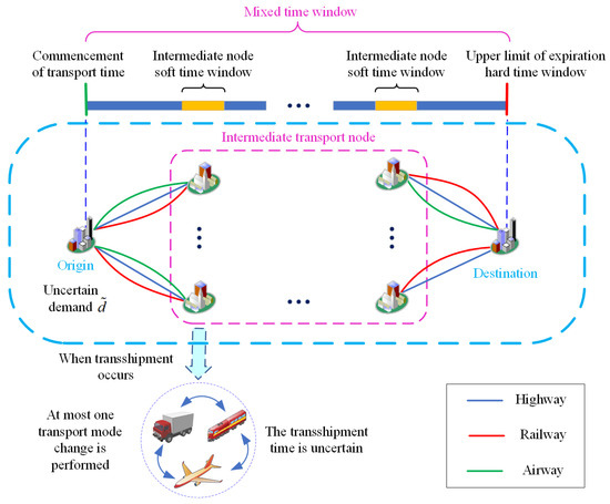
Figure 1.
Multimodal transport diagram.
The purpose of this study is to take transportation cost, transportation time, and transportation carbon emission as optimization objectives under the uncertain transportation environment and consider the mixed-time window constraint. In the specified time window, the obtained transportation path with the combination of nodes and transportation modes in the whole transportation process has the least total cost and the least carbon emission to provide a reliable path transportation scheme for multimodal transportation.
2.2. Fuzzy Demand Modeling
In this paper, fuzzy programming is used to describe the uncertainty of demand. The commonly used fuzzy numbers in fuzzy programming include triangular fuzzy number and trapezoidal fuzzy number. Compared with triangular fuzzy, trapezoidal fuzzy is more flexible in decision-making and can better match the actual decision-making situation [31]. Therefore, in this paper, the trapezoidal fuzzy number is used to represent the uncertainty of demand.
The trapezoidal fuzzy number uses four parameters to describe the uncertainty , as shown in Figure 2 [8]. Where is the most pessimistic estimate and is unlikely to happen in practice, but it could happen if things go badly. The interval indicates the lower and upper bounds of the most likely demand, corresponding to the most realistic scenario. is the most optimistic estimate, and like , it’s unlikely to happen in practice, but it’s possible when conditions are good.
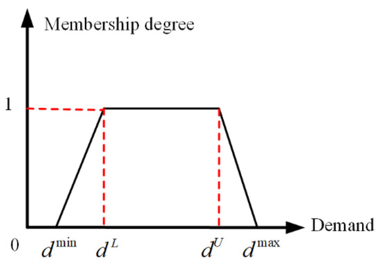
Figure 2.
The trapezoidal fuzzy number represents the fuzzy demand.
According to the four parameters of a trapezoidal fuzzy number, membership function of trapezoidal fuzzy number can be obtained, as shown in Equation (1) [32].
With the membership function of a trapezoidal fuzzy number, we can use it to describe the uncertainty of demand. In addition, the parameters of the membership function can be adjusted according to specific conditions to meet the requirements of actual application scenarios.
2.3. Multi-Objective Optimization Modeling of MULTIMODAL Transport
2.3.1. Parameter and Variable Definitions
In this paper, the parameters and variables defined in Table 1 are used to construct a multi-objective optimization model for multimodal transportation considering multiple uncertainty factors under a mixed-time window constraint.

Table 1.
Symbols and their representations.
2.3.2. Multi-Objective Optimization Model Construction Considering Mixed-Time Windows
To simplify the solution and optimization of the model, it is necessary to make some reasonable assumptions about the multimodal transport problem:
Assumption 1.
Goods can only be carried in a whole batch by one mode of transport between nodes and cannot be transported in parts.
Assumption 2.
The transfer of goods only takes place at the node city, and the mode of transport is changed at most once.
Assumption 3.
The path is acyclic, i.e., the same transport node can be passed at most once.
Assumption 4.
The transport time only considers the time between city nodes, not the micro time of intra-city transport.
Assumption 5.
The transport time obeys a normal distribution, i.e., , where is the average travel time between nodes and , i.e., , and denotes the standard deviation of the travel time between nodes and .
Assumption 6.
The transshipment time at the transshipment node obeys a uniform distribution, i.e., , where and denote the minimum and maximum values of the distribution, respectively.
Assumption 1 ensures that only one mode of transportation can be used during the transportation of goods and that no increase or decrease of goods will be generated; Assumption 2 ensures that at most one mode of transport changeover takes place when a transshipment of cargo occurs; Assumption 3 avoids repeated passage through the same node in the middle during path planning, which is consistent with the actual transportation situation; Assumption 4 makes the problem under study more concerned with path planning and simplifies the model processing; Assumption 5 describes the transportation time as a random variable following different normal distributions; Assumption 6 describes the transshipment time as a random variable following a uniform distribution to simulate realistic road conditions, weather, and other uncertainty factors.
These are the assumptions used in this paper, which simplify the model processing and problem-solving, and are closer to the actual transportation situation. Next, we will build a multi-objective optimization model for multimodal transportation based on these assumptions to solve the route planning problem considering multiple uncertainties under mixed time window constraints.
- Model objective function
The multimodal transport model established in this paper considers three optimization objectives: transportation cost, transportation time, and transportation carbon emission. Specifically, the total transportation cost includes transportation process cost, transshipment cost when a transshipment occurs, storage cost for early arrival, and penalty cost for late arrival, where the storage cost and penalty cost are caused by the violation of the soft time window of the intermediate node. Therefore, the transportation cost function can be expressed as:
The total transportation time includes the transportation process time and the transshipment time when transshipment occurs. Among them, the transport time obeys normal distribution, and the transshipment time at the transshipment node obeys uniform distribution. Therefore, the transport time function can be expressed by the following equation:
Transport carbon emissions are composed of carbon emissions in the transport process and transport carbon emissions during transport. The objective function of carbon emissions can be expressed as:
Equations (2)–(4) are the objective functions of the multi-objective optimization model of multimodal transport established in this paper.
- 2.
- Model Constraints
To ensure the correctness of the multimodal transport model solution results, some constraints must be imposed on the model. In this paper, the following constraints are set on the model:
(I) Time window constraint
In order to ensure the transportation time efficiency of cargo, reduce the cost, and improve the utilization of transportation resources, time window constraints need to be added to the model. In this paper, a mixed time window constraint is introduced, i.e., the time window of the intermediate node is set as a soft time window, which allows the cargo to arrive early or late, while the endpoint is set as a hard time window, in which the cargo must arrive within the range so that the model is more in line with the actual situation.
Constraint (5) represents the time for goods to arrive at place should satisfy the time window constraint at place . This is a soft time window constraint, where early arrival incurs storage costs and late arrival incurs penalty costs.
Constraint (6) is a hard time window constraint, which indicates that the total transportation time of the goods from the origin to the destination should be within the specified hard time window of the customer’s transportation order. Violation of this constraint is deemed as the transportation path is not feasible.
(II) Capacity constraints on transport and transshipment processes
When transporting between nodes, the volume of freight cannot exceed the range of transport capacity of the selected transport mode:
When transshipment occurs at a node, the volume of freight cannot exceed the transshipment capacity between the corresponding two modes of transport:
(III) Decision variable constraints
During transportation, only one mode of transportation can be selected between two adjacent nodes:
When a node transshipment occurs, at most one transshipment occurs:
Equations (2)–(10) construct a multi-objective optimization model for the multimodal transportation problem considering multiple uncertainty factors under the mixed time window constraint. The algorithm for solving this model will be presented in the next section of this paper.
3. Solution Method
3.1. Model Defuzzification
In Section 2, a fuzzy mixed-integer nonlinear programming model is developed in this paper, where the objective functions (2) and (4) and the constraints (7) and (8) carry trapezoidal fuzzy numbers indicating uncertain demands. Due to the uncertainty of these parameters, the model cannot be solved directly to obtain an optimal solution [23]. Therefore, to provide feasible route planning, the model needs to be de-fuzzified to obtain a clear model [4]. The process of defuzzification mainly includes two parts: defuzzification of objective function and defuzzification of fuzzy constraint.
3.1.1. Defuzzification of the Objective Function
The fuzzy expectation value model approach is an effective method for dealing with objective functions with fuzzy parameters [33]. The method uses the expected value of a fuzzy set to convert the fuzzy objective into a clear objective and achieves the objective de-fuzzification by minimizing or maximizing the expected value. By using the fuzzy expectation model, we can obtain a clear objective function that can better guide the actual decision.
In this paper, the objective functions (2) and (4) both involve the trapezoidal fuzzy number of uncertain demands, which makes it impossible to solve the objective function directly. Therefore, this paper uses the fuzzy expectation value model approach to defuzzify the objective functions (2) and (4) and rewrite them as Equations (11) and (12) to obtain a clear objective function.
where denotes the fuzzy expectation value of the fuzzy numbers in . Further, according to the linear property of the expected value operator, the Equations (11) and (12) can be converted to (13) and (14):
For a trapezoidal fuzzy number , its fuzzy expected value can be expressed as [34]:
Therefore, the objective function after defuzzification can be obtained by substituting Equation (15) into Equations (13) and (14), as shown in Equations (16) and (17):
Equations (16) and (17) are the de-fuzzy transportation cost and transportation time functions of the multimodal transport model. Compared with the original expressions (2) and (3), the defuzzification objective function is clearer and can be directly used for optimization and decision-making, allowing us to evaluate each route more accurately and thus provide a more feasible route planning solution.
3.1.2. Defuzzification of the Fuzzy Constraint
There are also two fuzzy constraints (7) and (8) in the model constraints constructed in Section 2. To solve these fuzzy constraints, we adopt a method that is widely used for fuzzy constraint problems in path planning, which is the fuzzy chance constraint planning method. By constructing the fuzzy chance constraint form, the fuzzy constraints are de-fuzzified, and finally, the de-fuzzified objective function is obtained.
In the fuzzy chance constraint planning method, the fuzzy measures of fuzzy events need to be determined first. Currently, there are three main fuzzy measures for modeling fuzzy chance constraints: possibility measure, necessity measure, and credibility measure [35]. Compared with the possibility and necessity measures, the credibility measure can more fully express the uncertainty, adapt to more complex solution scenarios, and has the property of self-dual, which provides convenience for the inverse operation of constraints often needed in practical problems. Therefore, this paper constructs a fuzzy chance constraint based on credibility measures. Based on the credibility measure, the fuzzy chance constraints of constraints (7) and (8) can be expressed as:
where represents the credibility of the fuzzy event in ; () is the confidence level set subjectively by the decision maker in the decision process based on knowledge, experience, and preference; and the fuzzy chance constraint ensures that the credibility of the fuzzy event should not be less than the confidence level. However, the description of the fuzzy events in is still related to the fuzzy parameters, and therefore still cannot be solved directly using the algorithm. The literature [36] provides a clear expression to measure the confidence that the trapezoidal fuzzy number is not less than the deterministic number. For a trapezoidal fuzzy number and a deterministic number , when a fuzzy credibility measure is used, there is the following relation:
In practical decision-making, the confidence level is usually set in the interval [37], and therefore, based on the segmented linear relationship of the confidence measure (Figure 3), can be rewritten as:
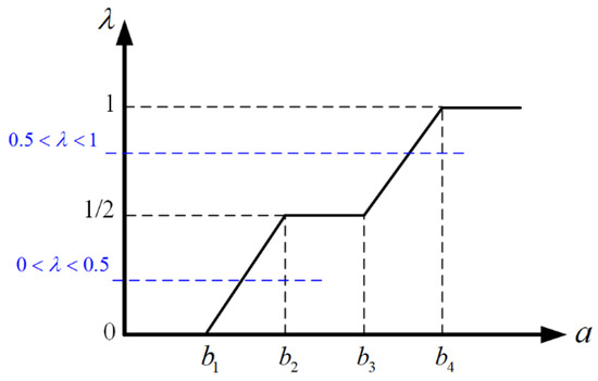
Figure 3.
Credibility measure segmented linear relationship.
According to (21), the equivalently clear form of the chance constraint of Equations (18) and (19) can be obtained as follows:
After the fuzzy object and fuzzy constraint are de-fuzzified, clear and explicit objective functions and constraints are obtained, which makes the model solution more specific and easier. Next, the algorithm used to solve the multi-objective model of multimodal transportation will be introduced in this paper.
3.2. Design of Multimodal Transport Route Optimization Algorithm
The multimodal transport model proposed in this paper is a multi-objective optimization model, which needs to integrate users’ preferences for each objective to determine a single suitable solution. The weighted sum method is a classical algorithm to deal with multi-objective models, especially preference models, and its effectiveness in solving multi-objective models has been proven. This method combines the user’s preferences for various targets, converts the multi-objective model to the single objective model by specifying the weight of the target, and keeps the weights constant to obtain a suitable solution by algorithmic solution. In this paper, since the objective functions (2), (3), and (4) contain variables of different units, respectively, they must be dimensionless before converting them to single objective functions [38]:
where are the maximum values of the total cost, total time, and carbon emission, respectively. are the minimum values of the total cost, total time, and carbon emissions, respectively. The dimensionless multi-objective model can then be weighted and summed to a single-objective model by Equation (25):
where represents the generalized cost function weighted by each objective. represents the weighting factors of different objectives.
3.2.1. Dynamic Optimization of Multi-Objective Weights Based on Game Theory Approach
The weighted sum method can transform the multi-objective model into a single-objective model, which is convenient for the algorithm to solve. However, it is often difficult to avoid subjectivity in setting the weight coefficient of multiple objectives, and it is difficult to determine the appropriate weight of different objectives according to preferences. The fixed weight makes the optimal solution of optimization abandon the benefits of the whole system, causing unnecessary losses. Therefore, this paper proposes a multi-objective optimization method for multimodal transportation based on cooperative game theory, which makes each objective as far as possible from the worst value of all individual objectives and seeks the equilibrium weights between each objective without a priori knowledge through cooperative game theory [39]. In the optimization process of using the algorithm, the weight of each object is constantly adjusted dynamically to obtain the best multimodal transportation routing solution. The dynamic optimization process of multi-objective weights based on the cooperative game theory approach is as follows:
Firstly, each optimization objective is minimized separately, and the values of each objective under the optimal solution obtained when minimizing each objective are recorded. From all the recorded values, determine the minimum and worst values of objective .
Next, the model is solved using the optimization algorithm, and the value of each objective obtained by each optimization algorithm is normalized using Equation (26). The normalized value of 0 indicates that the objective reaches its optimal value, and the normalized value of 1 indicates that the objective reaches its worst value.
Finally, define the combined objective (Equation (27)) and update the weights of all objectives optimized by minimizing the combined objective .
where represent the cost, time, and carbon emission objectives optimized in the model, respectively, and is a supernormal value introduced as a penalty to avoid each objective being too close to its worst case.
Through the above method, the weights of each object in the method can be dynamically adjusted in the process of algorithm optimization. The weights of each objective are set as equal at the initialization and then updated dynamically and iteratively by the cooperative game theory method.
3.2.2. Solving Multimodal Transport Models Based on PSO Optimization
After the weight of each object is updated dynamically by the cooperative game theory method, the PSO algorithm is used to optimize the multimodal transport model. The PSO algorithm adjusts two properties of itself: position () and velocity (), based on the individual extremes value () and global extremes value () of the particle trajectories in the search space, and converges to the global optimal solution through continuous iterative updates. In this paper, each particle represents a transport path. Assuming that the particle search space is D dimension, the velocity and position update formula of each particle in dimension d in the n-th iteration is as follows:
where is the inertia factor, and are random numbers on the interval , and and are the learning factors, which are set to 2.05 and 2.05, respectively [40]. To balance the global and local search performance of PSO and reduce the number of iterations, the linear decreasing weight strategy (LDW) [41] is used in this paper to update the inertia factor .
where is the initial inertia weight, is the inertia weight at the maximum number of iterations, is the current number of iterations, and is the maximum number of iterations. According to the literature [42], = 0.9 and = 0.4 are taken.
In summary, the specific implementation steps of the cooperative game theory-based multi-objective optimization method for multimodal transport proposed in this paper are as follows:
Step 1: Minimize each objective separately and obtain the optimal value and the worst value for the -th objective.
Step 2: Initialize the weights and convert the multi-objective problem to a single-objective problem using the weighted sum method.
Step 3: in Equation (25) is used as the cost function of the PSO, the current optimal solution is obtained by optimization, and the value of each objective is recorded.
Step 4: The values of each objective obtained from the solution of the optimization algorithm are normalized, and the weights of each objective are dynamically adjusted by the cooperative game theory method using Equation (27).
Step 5: Determine whether the termination condition is satisfied (the maximum number of iterations G is reached). If not, return to Step 3 to continue optimization; if yes, obtain the optimal path by comparing all the recorded paths.
During the iterative process, the objective weights are dynamically adjusted by the cooperative game theory approach, and the solution space is extensively searched. The PSO algorithm is used to optimize the solution, optimize the value of the objective function, and select the best solution while under the guidance of the cooperative game theory method. The algorithm finds the optimal path for the multimodal transportation model in the tradeoffs exploration and exploitation described above.
The flow chart of the designed cooperative game theory-based multi-objective dynamic optimization method for multimodal transport is shown in Figure 4.
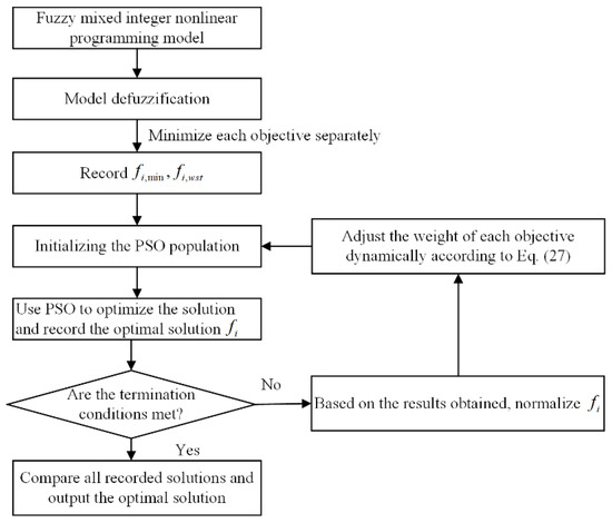
Figure 4.
Multi-objective dynamic optimization method for multimodal transport based on cooperative game theory.
4. Empirical Case Study
4.1. Case Description
In this section, a study is conducted with a real intermodal network of KYE Company in China to verify the effectiveness of the proposed method and further discuss the impact of uncertain demand and time on multimodal route optimization problems with time windows. Through case studies, practical path-planning suggestions and options are provided for decision-makers.
KYE is a large modern, integrated express transportation company mainly engaged in “limited time express” service and has established a strong logistics business system in China with rich transportation experience and advantages of land and air resources. Considering the geographical and economic distributions, this paper selects part of its intermodal network in mainland China for research, and the transportation network is shown in Figure 5. As an important logistics distribution node, Guangzhou is selected as an intermodal originating city to transport a batch of cargo to Beijing, a northern city in China. According to the investigation of KYE’s operation data, the cargo demand in this paper is expressed by trapezoidal fuzzy numbers as = (8t, 12t, 18t, 22t).
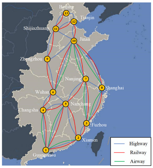
Figure 5.
Multimodal transportation network in the empirical case.
According to the actual situation, there are three modes of transportation in this multimodal transportation network: highway, railway, and airway. The transportation distances of different transportation modes between nodes are shown in Table 2. Among them, the road distance is obtained through Gaode Map (One of the most popular map service providers in China), the railroad distance is obtained through the website of China Railway 12306, and the air distance is derived by referring to the flight mileage of Southern Airlines.
Table 2.
Transportation distance between transportation nodes.
The average speed, unit transportation cost, and unit transportation carbon emission of various transportation modes are shown in Table 3. The data are obtained from studies in the literature [14,43,44] and others. The transport time obeys a normal distribution of , where is the average travel time between nodes and , i.e.,, taking the standard deviation .
Table 3.
Transport-related parameters.
The unit transshipment cost and carbon emission per unit transshipment between various transportation modes are shown in Table 4, with data referenced from the literature [14,44] and actual operational data from KYE. The transshipment time between the various modes of transportation obeys a uniform distribution and .
Table 4.
Transshipment parameters.
The transport capacity between each node and the transfer capacity between different modes at the transshipment nodes are shown in Table 5 and Table 6.
Table 5.
Transport capacity between nodes (Unit: t).
Table 6.
Transfer capacity at the nodes (Unit: t).
In China, packages usually arrive within three days. In this paper, the upper limit of the hard time window of shipping time is set to 72 h. For the convenience of modeling and calculation, the planning range from 0:00 on day 1 to 24:00 on day 3 is converted to the range [0, 72 h]. Therefore, the time window constraints for each node are shown in Table 7.
Table 7.
Time window of the nodes (Unit: h).
According to KYE’s survey data, the unit storage cost incurred by the early arrival of goods is CNY 30/(t∙h), and the unit penalty cost for late arrival is CNY 50/(t∙h). In addition, the confidence level in the fuzzy chance constraint has a significant effect on the multimodal optimization results, and according to [5,34] et al., the confidence degree is taken. Next, this paper will verify the effectiveness of the proposed algorithm in this real intermodal network case and further discuss the impact of uncertainties on multimodal route optimization.
4.2. Result Analysis
In this section, the effectiveness of the cooperative game theory-based multi-objective optimization method for multimodal transportation is verified by the case in 4.1, and the impact of uncertainty on path planning is discussed. All algorithms are based on MATLAB R2021b running under Windows 10 (64-bit) with a Core i5 CPU and 8 GB RAM.
4.2.1. Algorithm Validity
To verify the effectiveness of cooperative game theory in dynamically adjusting the weights of each objective in the process of algorithm optimization, this paper compares the weighted sum method based on cooperative game theory with the weighted sum method using fixed weights. Using the fixed-weight weighted sum method, four different weight combinations are tested:
I. (1, 1, 1).
II. (0.8, 0.1, 0.1).
III. (0.1, 0.8, 0.1).
IV. (0.1, 0.1, 0.8).
In brackets, cost, time, and carbon emission weighting factors are in order. The four combinations represent equal weight, cost preference, time preference, and carbon emission preference, respectively. The weighted sum method based on cooperative game theory is represented by V. For each combination of weights, the PSO algorithm population size is 20, and the maximum number of iterations is 200, and the results of the runs are obtained as shown in Table 8. Better results in the table are shown in bold. Also, to visually compare the optimization results of each objective when using different weights, the data in Table 8 are represented in Figure 6.
Table 8.
Comparison results of different weighting combinations.
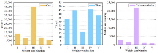
Figure 6.
Comparison results of different weighting combinations.
According to the results in Table 8 and Figure 6, it can be seen that the results of dynamically adjusting the weight of each objective through cooperative game theory are better than those of using fixed weight combinations on the whole. Each objective is well away from its worst result and effectively finds the optimal solution. This proves that the method of dynamically adjusting weights by cooperative game theory effectively improves the performance of the weighted sum method.
Meanwhile, under the multi-objective model, different combinations of objective weights can lead to different transportation solutions, and an inappropriate setting of an objective weight can damage the whole system. For example, with the enhanced preference for the time objective (weight combination III), although transport time is greatly reduced, transport costs and transport carbon emissions increase sharply, which seriously harms the interests of carriers and the environment and is not in line with the green transportation concept.
In this paper, we set the maximum number of update iterations G = 200 for dynamically adjusting the weights of each objective using game theory, and the process of dynamically adjusting the weights is shown in Figure 7. It can be seen that during the optimization process, the weights of each objective are dynamically updated and stabilized in a certain range; that is, the weighted sum method based on cooperative game theory has cost, time, and carbon emission weighting factors varying in the range of (0.20~0.45, 0.36~0.70, 0.07~0.27), showing the relevant equilibrium among the objectives of the game process, and the algorithm has the optimal solution in this dynamic optimization.
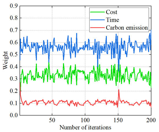
Figure 7.
Cooperative game theory dynamic adjustment weighting process.
In addition, the weighted sum method based on cooperative game theory (CGT-WSM) is compared with multi-objective particle swarm optimizer (MOPSO) and non-dominated sorting Genetic Algorithm-II (NSGA-II) to verify the effectiveness of the proposed method in solving multi-objective optimization models for multimodal transport. Where the population size of the MOPSO algorithm is 50, the maximum number of iterations is 200, the learning factors are both 2.05, the initial and final inertia weights are 0.9 and 0.4, respectively, and the Pareto solution set library is 30. The population size of the NSGA-II algorithm is 50, the maximum number of iterations is 200, and the crossover rate is 0.7, which is used to control the probability that an offspring individual inherits genes from a parent individual. A higher crossover rate helps maintain population diversity and facilitates global search. A variation rate of 0.4 is used to introduce randomness and help jump out of local optima. A higher variation rate helps to explore the search space and potentially discover new solutions. The set of Pareto optimal solutions obtained by the three methods is shown in Figure 8, Figure 9 and Figure 10.
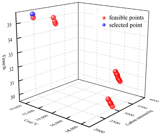
Figure 8.
MOPSO Pareto optimal solution set.
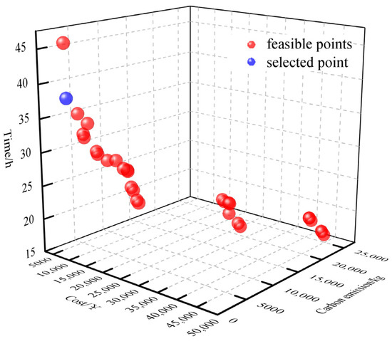
Figure 9.
NSGA-II Pareto optimal solution set.
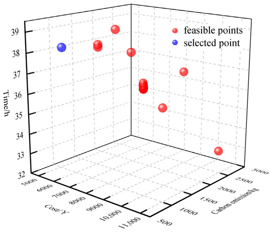
Figure 10.
CGT-WSM Pareto optimal solution set.
The Pareto optimal solution of the model obtained using MOPSO and NSGA-II is a non-dominated set of solutions, so it is also necessary to combine the decision maker’s preferences for each objective to determine the final solution. As mentioned in Section 2.1, the purpose of this study is to obtain the transportation path with the least total transportation cost and the least carbon emission in the uncertain transportation environment within the specified time window. According to the analysis of the Pareto optimal solution sets of MOPSO and NSGA-II, it is found that the total transportation time of all solutions is within the specified time window (72 h), and all of them are feasible solutions. Therefore, the total cost and carbon emissions are further analyzed, and the optimal solutions of MOPSO and NSGA-II algorithms are finally determined, as shown in the blue points in Figure 8 and Figure 9. The comparison of the results obtained with the weighted sum method based on cooperative game theory (CGT-WSM) is shown in Table 9. Better results in the table are shown in bold.
Table 9.
Comparison of algorithm optimization results.
According to the algorithm comparison results, it can be seen that the paths obtained by the three methods are the same, but the transportation modes are different. In the specified time window, the proposed weighted sum method based on cooperative game theory requires a lower cost compared to MOPSO and NSGA-II and can combine the decision maker’s preference for the objective well to obtain the optimal path that satisfies the time window requirement. The effectiveness of the weighted sum method in the multi-objective preference model is further proved.
To further compare the performance of the three algorithms, this paper compares the hypervolume (HV) and inverted generational distance (IGD) [22] of the MOPSO, NSGA-II, and CGT-WSM algorithms for multimodal path optimization problems to assess the differences between these algorithms in terms of diversity, distributivity, and approximation of the true frontier. Each algorithm is executed independently 20 times to collect statistics, and the results obtained are shown in Table 10. Better results in the table are shown in bold.
Table 10.
Mean and sd of HV and IGD of MOPSO, NSGA-II, and CGT-WSM.
Table 10 shows that the CGT-WSM algorithm is slightly lower than the MOPSO and NSGA-II algorithms in terms of the mean value of HV, but its standard deviation of HV and the mean and standard deviation of IGD are smaller than the other two algorithms. These results show that the solution set of the CGT-WSM algorithm performs well in approximating the optimal solution while ensuring good diversity and performs better in the distribution consistency of the solution set and approximating the real frontier. The above results imply that the CGT-WSM algorithm maintains a good balance between exploration and exploitation. Although the HV value of its solution set is slightly smaller, its better stability and performance close to the real frontier enable the CGT-WSM algorithm to provide better approximate solutions in problem-solving.
To determine if there is a significant difference in performance between these algorithms, we chose to perform a non-parametric hypothesis test at the 5% significance level. In this paper, Kruskal–Wallis one-way ANOVA [45] is used as a nonparametric hypothesis testing method because of its applicability in comparing the equality of distributions of multiple independent samples. The following research hypotheses are first proposed:
H0 (null hypothesis):
there is no significant difference between the three multi-objective algorithms.
H1 (Alternative hypothesis):
there is a significant difference between the performance of the three multi-objective algorithms.
By performing the Kruskal–Wallis test, we calculated p = 1.63 × 10⁻⁵, which is much less than the significance level. Therefore, it means that at a 5% level of significance, we can reject the null hypothesis and conclude that there is a significant difference between the three multi-objective algorithms.
4.2.2. Analysis of the Impact of Uncertainty
To analyze the impact of uncertainty factors on multimodal transport route planning, the following four transport scenarios are considered in this paper:
Scenario I. Determined demand and determined time.
Scenario II. Uncertain demand and determined time.
Scenario III. Determined demand and uncertain time.
Scenario IV. Uncertain demand and uncertain time.
When using the weighted sum method to optimize each transportation scenario, to facilitate the comparison of the influence of uncertain factors on optimization results, the weight of each objective is taken as the average value of the dynamic optimization process of game theory, namely = (0.33, 0.57, 0.10). The optimization results of various transportation scenarios are shown in Table 11.
Table 11.
Optimization results for different transportation scenarios.
Figure 11 shows the results of the comparison of cost, time, and carbon emissions for four different transportation scenarios.
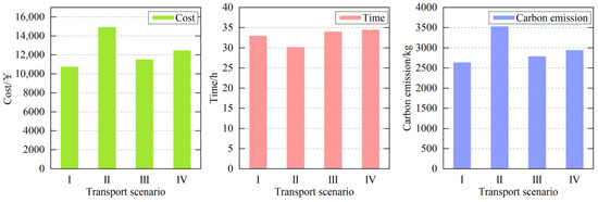
Figure 11.
Comparison of optimization results of different transportation scenarios.
- (1)
- When the conditions of time factor are the same, the uncertainty of demand will lead to an increase in transportation cost and carbon emission and have some influence on the transportation time. When the time factors are determined, the cost of Scenario II increases by 39.0%, the carbon emission increases by 34%, and the time decreases by 9.44% compared to Scenario I. When the time factors are uncertain, Scenario IV increases the cost by 8.27%, carbon emission by 5.57%, and time by 1.74% compared to Scenario III.
- (2)
- When the demand factor conditions are the same, the uncertainty of time leads to a slight increase in transportation time and has some impact on transportation costs and carbon emissions. When the demand factors are deterministic, Scenario III increases costs by 7.30%, carbon emissions by 5.82%, and time by 2.85% compared to Scenario I. When the demand factors are uncertain, Scenario IV has 16.42% less cost, 16.66% less carbon emissions, and 14.52% more time than Scenario II.
- (3)
- According to the analysis of the results in (1) and (2), demand uncertainty has a more significant impact on the optimization results of the multimodal transport model. When the time factors are determined, demand uncertainty increases transportation costs and carbon emissions significantly, whereas when the demand factors are determined, time uncertainty increases the transportation time but has insignificant effects on transportation costs and carbon emissions.
According to the above analysis, uncertain factors will increase transportation costs and carbon emissions and affect the choice of routes and transportation modes. Therefore, it is necessary to consider the uncertainty factor in the model when performing multimodal transport route planning. By taking uncertainties into account, the robustness and accuracy of route planning results can be improved, thus providing a more reliable and efficient solution for multimodal transport services.
5. Conclusions and Future Work
In this paper, a multi-objective fuzzy nonlinear programming model considering mixed time window constraints is established to solve the problem of multimodal transport path planning under an uncertain environment, taking cost, time, and carbon emission as optimization objectives. Then, the fuzzy expected value method and the fuzzy chance-constrained programming method are used to de-fuzzify the multi-objective fuzzy programming model, and the deterministic parameters of the model are obtained. To solve the model, a multi-objective optimization method of multimodal transport based on cooperative game theory is proposed. The game theory method is combined with the weighted sum method, and the weight of each objective is dynamically adjusted in the algorithm optimization process through cooperative game theory to obtain the optimal multimodal transport path. Finally, the effectiveness of the proposed algorithm is verified in a real combined transport network.
The experiment results show that the method of dynamically adjusting weights by cooperative game theory effectively improves the performance of the weighted sum method, and the obtained results are overall better than those using a fixed combination of weights. In addition, compared with MOPSO and NSGA-II, the proposed algorithm has a better optimization effect and can combine the decision-makers’ preference for the goal well to obtain the optimal path that meets the requirements of the time window, effectively reducing transportation costs and carbon emissions and promoting the development of green transportation. The effectiveness of the weighted sum method in the multi-objective preference model is further proved.
Finally, this paper analyzes the influence of uncertainty factors on multimodal route planning results. The results show that demand uncertainty has a more obvious influence on the optimization results of the multimodal transport model than time uncertainty. It is necessary to consider the uncertainty factor in the model when performing multimodal transport route planning. By taking uncertainties into account, the robustness and accuracy of route planning results can be improved, thus providing a more reliable and efficient solution for multimodal transport services.
In addition, through the analysis of route optimization results, it can be seen that railway transportation plays a significant role in reducing transportation costs and carbon emissions. Therefore, in future work, we will further explore the impact of the railway on the multimodal transport structure, and we will consider more uncertainty factors in the model to better simulate the real transportation environment, as well as find other methods to solve the multi-objective problem and provide more reliable multimodal transportation path solutions.
Author Contributions
L.L.: Methodology, Writing—reviewing and editing, Supervision, Investigation. Q.Z.: Methodology, Formal analysis, Software, Data curation, Writing—original draft, Writing—reviewing and editing. T.Z.: Validation, Project administration, Funding acquisition, Writing—reviewing and editing. Y.Z.: Conceptualization, Data curation, Software, Supervision. X.Z.: Investigation, Data curation, Validation. All authors have read and agreed to the published version of the manuscript.
Funding
This research was funded by the Department of Science and Technology of Guangdong Province, grant number 2021B0101420003.
Data Availability Statement
We created a dataset for this study. Since further research is in progress, we cannot publish the dataset right now.
Conflicts of Interest
The authors declare no conflict of interest.
References
- Chen, M.F.; Liu, Y.Q.; Song, Y.; Sun, Q.; Cong, C.C. Multimodal Transport Network Optimization Considering Safety Stock under Real-Time Information. Discret. Dyn. Nat. Soc. 2019, 2019, 5480135. [Google Scholar] [CrossRef]
- Ji, S.F.; Luo, R.J. A Hybrid Estimation of Distribution Algorithm for Multi-Objective Multi-Sourcing Intermodal Transportation Network Design Problem Considering Carbon Emissions. Sustainability 2017, 9, 1133. [Google Scholar] [CrossRef]
- Rudi, A.; Fröhling, M.; Zimmer, K.; Schultmann, F. Freight transportation planning considering carbon emissions and in-transit holding costs: A capacitated multi-commodity network flow model. EURO J. Transp. Logist. 2016, 5, 123–160. [Google Scholar] [CrossRef]
- Tian, W.L.; Cao, C.X. A generalized interval fuzzy mixed integer programming model for a multimodal transportation problem under uncertainty. Eng. Optim. 2017, 49, 481–498. [Google Scholar] [CrossRef]
- Sun, Y.; Hrusovsky, M.; Zhang, C.; Lang, M.X. A Time-Dependent Fuzzy Programming Approach for the Green Multimodal Routing Problem with Rail Service Capacity Uncertainty and Road Traffic Congestion. Complexity 2018, 2018, 8645793. [Google Scholar] [CrossRef]
- Ramezani, M.; Bashiri, M.; Tavakkoli-Moghaddam, R. A new multi-objective stochastic model for a forward/reverse logistic network design with responsiveness and quality level. Appl. Math. Model. 2013, 37, 328–344. [Google Scholar] [CrossRef]
- Sun, Y. Fuzzy Approaches and Simulation-Based Reliability Modeling to Solve a Road-Rail Intermodal Routing Problem with Soft Delivery Time Windows When Demand and Capacity are Uncertain. Int. J. Fuzzy Syst. 2020, 22, 2119–2148. [Google Scholar] [CrossRef]
- Zarandi, M.H.F.; Hemmati, A.; Davari, S. The multi-depot capacitated location-routing problem with fuzzy travel times. Expert Syst. Appl. 2011, 38, 10075–10084. [Google Scholar] [CrossRef]
- Baykasoglu, A.; Subulan, K. A fuzzy-stochastic optimization model for the intermodal fleet management problem of an international transportation company. Transp. Plan. Technol. 2019, 42, 777–824. [Google Scholar] [CrossRef]
- Demir, E.; Burgholzer, W.; Hrušovský, M.; Arıkan, E.; Jammernegg, W.; Van Woensel, T. A green intermodal service network design problem with travel time uncertainty. Transp. Res. Part B Methodol. 2016, 93, 789–807. [Google Scholar] [CrossRef]
- Zhao, Y.; Liu, R.H.; Zhang, X.; Whiteing, A. A chance-constrained stochastic approach to intermodal container routing problems. PLoS ONE 2018, 13, e0192275. [Google Scholar] [CrossRef]
- Lu, Y.; Lang, M.; Yu, X.; Li, S. A sustainable multimodal transport system: The two-echelon location-routing problem with consolidation in the Euro–China expressway. Sustainability 2019, 11, 5486. [Google Scholar] [CrossRef]
- Chen, C.; Demir, E.; Huang, Y. An adaptive large neighborhood search heuristic for the vehicle routing problem with time windows and delivery robots. Eur. J. Oper. Res. 2021, 294, 1164–1180. [Google Scholar] [CrossRef]
- Zheng, C.J.; Sun, K.; Gu, Y.H.; Shen, J.X.; Du, M.Q. Multimodal Transport Path Selection of Cold Chain Logistics Based on Improved Particle Swarm Optimization Algorithm. J. Adv. Transp. 2022, 2022, 5458760. [Google Scholar] [CrossRef]
- Zhang, Y.; Hua, G.W.; Cheng, T.C.E.; Zhang, J.L. Cold chain distribution: How to deal with node and arc time windows? Ann. Oper. Res. 2020, 291, 1127–1151. [Google Scholar] [CrossRef]
- Chang, Y.-T.; Lee, P.T.-W.; Kim, H.-J.; Shin, S.-H. Optimization model for transportation of container cargoes considering short sea shipping and external cost: South Korean case. Transp. Res. Rec. 2010, 2166, 99–108. [Google Scholar] [CrossRef]
- Vale, C.; Ribeiro, I.M. Intermodal routing model for sustainable transport through multi-objective optimization. In Proceedings of the 2nd EAI International Conference on Intelligent Transport Systems (INTSYS), Guimaraes, Portugal, 21–23 November 2018; pp. 144–154. [Google Scholar] [CrossRef]
- Sun, Y. Green and Reliable Freight Routing Problem in the Road-Rail Intermodal Transportation Network with Uncertain Parameters: A Fuzzy Goal Programming Approach. J. Adv. Transp. 2020, 2020, 7570686. [Google Scholar] [CrossRef]
- Heinold, A.; Meisel, F. Emission limits and emission allocation schemes in intermodal freight transportation. Transp. Res. Part E-Logist. Transp. Rev. 2020, 141, 101963. [Google Scholar] [CrossRef]
- Zheng, H.-y.; Wang, L. Reduction of carbon emissions and project makespan by a Pareto-based estimation of distribution algorithm. Int. J. Prod. Econ. 2015, 164, 421–432. [Google Scholar] [CrossRef]
- Marler, R.T.; Arora, J.S. The weighted sum method for multi-objective optimization: New insights. Struct. Multidiscip. Optim. 2010, 41, 853–862. [Google Scholar] [CrossRef]
- Majumder, S.; Kar, S.; Pal, T. Mean-entropy model of uncertain portfolio selection problem. In Multi-Objective Optimization: Evolutionary to Hybrid Framework; Springer: Berlin/Heidelberg, Germany, 2018; pp. 25–54. [Google Scholar] [CrossRef]
- Wang, R.; Yang, K.; Yang, L.X.; Gao, Z.Y. Modeling and optimization of a road-rail intermodal transport system under uncertain information. Eng. Appl. Artif. Intell. 2018, 72, 423–436. [Google Scholar] [CrossRef]
- Li, H.X.; Wang, S.W. Model-based multi-objective predictive scheduling and real-time optimal control of energy systems in zero/low energy buildings using a game theory approach. Autom. Constr. 2020, 113, 103139. [Google Scholar] [CrossRef]
- Li, X.Y.; Gao, L.; Li, W.D. Application of game theory based hybrid algorithm for multi-objective integrated process planning and scheduling. Expert Syst. Appl. 2012, 39, 288–297. [Google Scholar] [CrossRef]
- Chen, X.H.; Zuo, T.S.; Lang, M.X.; Li, S.Q.; Li, S.Y. Integrated optimization of transfer station selection and train timetables for road-rail intermodal transport network. Comput. Ind. Eng. 2022, 165, 107929. [Google Scholar] [CrossRef]
- Peng, Y.; Yong, P.C.; Luo, Y.J. The route problem of multimodal transportation with timetable under uncertainty: Multi-objective robust optimization model and heuristic approach. Rairo-Oper. Res. 2021, 55, S3035–S3050. [Google Scholar] [CrossRef]
- Marinakis, Y.; Migdalas, A.; Sifaleras, A. A hybrid Particle Swarm Optimization—Variable Neighborhood Search algorithm for Constrained Shortest Path problems. Eur. J. Oper. Res. 2017, 261, 819–834. [Google Scholar] [CrossRef]
- Deng, L.X.; Chen, H.Y.; Zhang, X.Y.Q.; Liu, H.Y. Three-Dimensional Path Planning of UAV Based on Improved Particle Swarm Optimization. Mathematics 2023, 11, 1987. [Google Scholar] [CrossRef]
- Singh, N.; Singh, S.B.; Houssein, E.H. Hybridizing salp swarm algorithm with particle swarm optimization algorithm for recent optimization functions. Evol. Intell. 2022, 15, 23–56. [Google Scholar] [CrossRef]
- Sun, Y.; Zhang, G.; Hong, Z.; Dong, K. How uncertain information on service capacity influences the intermodal routing decision: A fuzzy programming perspective. Information 2018, 9, 24. [Google Scholar] [CrossRef]
- Yan, S.; Maoxiang, L.; Jiaxi, W. On solving the fuzzy customer information problem in multicommodity multimodal routing with schedule-based services. Information 2016, 7, 13. [Google Scholar] [CrossRef]
- Kundu, P.; Kar, S.; Maiti, M. Multi-objective multi-item solid transportation problem in fuzzy environment. Appl. Math. Model. 2013, 37, 2028–2038. [Google Scholar] [CrossRef]
- Sun, Y.; Liang, X.; Li, X.Y.; Zhang, C. A Fuzzy Programming Method for Modeling Demand Uncertainty in the Capacitated Road-Rail Multimodal Routing Problem with Time Windows. Symmetry-Basel 2019, 11, 91. [Google Scholar] [CrossRef]
- Vahdani, B.; Tavakkoli-Moghaddam, R.; Jolai, F.; Baboli, A. Reliable design of a closed loop supply chain network under uncertainty: An interval fuzzy possibilistic chance-constrained model. Eng. Optim. 2013, 45, 745–765. [Google Scholar] [CrossRef]
- Habib, M.S.; Asghar, O.; Hussain, A.; Imran, M.; Mughal, M.P.; Sarkar, B. A robust possibilistic programming approach toward animal fat-based biodiesel supply chain network design under uncertain environment. J. Clean. Prod. 2021, 278, 122403. [Google Scholar] [CrossRef]
- Zhu, H.; Zhang, J. A credibility-based fuzzy programming model for APP problem. In Proceedings of the 2009 International Conference on Artificial Intelligence and Computational Intelligence, Shanghai, China, 7–8 November 2009; pp. 455–459. [Google Scholar] [CrossRef]
- Han, B.; Shi, S.S.; Gao, H.T.; Hu, Y. A Sustainable Intermodal Location-Routing Optimization Approach: A Case Study of the Bohai Rim Region. Sustainability 2022, 14, 3987. [Google Scholar] [CrossRef]
- Mahjoubi, S.; Bao, Y. Game theory-based metaheuristics for structural design optimization. Comput. -Aided Civ. Infrastruct. Eng. 2021, 36, 1337–1353. [Google Scholar] [CrossRef]
- Cheng, X.Z.; Li, J.M.; Zheng, C.Y.; Zhang, J.H.; Zhao, M. An Improved PSO-GWO Algorithm With Chaos and Adaptive Inertial Weight for Robot Path Planning. Front. Neurorobot. 2021, 15, 770361. [Google Scholar] [CrossRef]
- Arasomwan, M.A.; Adewumi, A.O. On the Performance of Linear Decreasing Inertia Weight Particle Swarm Optimization for Global Optimization. Sci. World J. 2013, 2013, 860289. [Google Scholar] [CrossRef]
- Chrouta, J.; Farhani, F.; Zaafouri, A. A modified multi swarm particle swarm optimization algorithm using an adaptive factor selection strategy. Trans. Inst. Meas. Control. 2021, 3, 01423312211029509. [Google Scholar] [CrossRef]
- Resat, H.G.; Turkay, M. Design and operation of intermodal transportation network in the Marmara region of Turkey. Transp. Res. Part E-Logist. Transp. Rev. 2015, 83, 16–33. [Google Scholar] [CrossRef]
- Zhang, H.; Li, Y.; Zhang, Q.P.; Chen, D.J. Route Selection of Multimodal Transport Based on China Railway Transportation. J. Adv. Transp. 2021, 2021, 9984659. [Google Scholar] [CrossRef]
- Wan, X.L.; Yamada, Y. An Acceleration-Based Nonlinear Time-Series Analysis of Effects of Robotic Walkers on Gait Dynamics During Assisted Walking. IEEE Sens. J. 2022, 22, 21188–21196. [Google Scholar] [CrossRef]


Disclaimer/Publisher’s Note: The statements, opinions and data contained in all publications are solely those of the individual author(s) and contributor(s) and not of MDPI and/or the editor(s). MDPI and/or the editor(s) disclaim responsibility for any injury to people or property resulting from any ideas, methods, instructions or products referred to in the content. |
© 2023 by the authors. Licensee MDPI, Basel, Switzerland. This article is an open access article distributed under the terms and conditions of the Creative Commons Attribution (CC BY) license (https://creativecommons.org/licenses/by/4.0/).