Fuzzy Analytic Network Process with Principal Component Analysis to Establish a Bank Performance Model under the Assumption of Country Risk

Abstract

In recent years, bank-related decision analysis has reflected a relevant research area due to key factors that affect the operating environment of banks. This study’s aim is to develop a model based on the linkages between the performance of banks and their operating context, determined by country risk. For this aim, we propose a multi-analytic methodology using fuzzy analytic network process (fuzzy-ANP) with principal component analysis (PCA) that extends existing mathematical methodologies and decision-making approaches. This method was examined in two studies. The first study focused on determining a model for country risk assessment based on the data extracted from 172 countries. Considering the first study’s scores, the second study established a bank performance model under the assumption of country risk, based on data from 496 banks. Our findings show the importance of country risk as a relevant bank performance dimension for decision makers in establishing efficient strategies with a positive impact on long-term performance. The study offers various contributions. From a mathematic methodology perspective, this research advances an original approach that integrates fuzzy-ANP with PCA, providing a consistent and unbiased framework that overcomes human judgement. From a business and economic analysis perspective, this research establishes novelty based on the performance evaluation of banks considering the operating country’s risk.

1. Introduction

Worldwide, there are increasing concerns based on political and economic unrest. Escalating geopolitical differences in various areas of the world, international threat of financial crisis and economic downturn, increasing income inequality, and many other factors affect the operating environment of banks. Globalization enhances the propagation of these factors based on the interconnectedness of “economic structures, financial markets, and political institutions” [1], thus increasing the urgency of examining country risk and its connection to bank performance.

Initial investigations have described country risk as the potential incapacity of a sovereign state to generate sufficient foreign exchange to reimburse its external debt [2,3,4]. Explaining the primary “risk factors, causes, levels, and development trends” in a country or region represents the main goal of country risk investigation and assessment [4]. As a multifaceted topic, previous empirical investigations have explored country risk in relation to various contexts, such as environmental issues [5,6,7,8,9], supply chain contexts [10,11,12], and energy [13,14], as well as business contexts related to process effectiveness [15] and firm exposure [16].

Country risk has also proven to be highly relevant in assessing performance and related activities of banks and financial institutions [1,17,18,19,20]. To examine country risk and its potential impact on business operations, previous empirical investigations have used a wide range of data analysis techniques, such as Copula [21], regression [6,7,8,10,14,16,17], analytic hierarchy process (AHP) [15], fuzzy sets [8,15,22], Bayesian Belief Network [11], Grey-TOPSIS Model [23], artificial neural networks [24], and principal component analysis [12,25,26]. Nonetheless, no consensus has been reached in proposing a specific methodology and framework. Therefore, it is of great significance to further develop new methodologies and data analysis techniques to assess country risk and evaluate bank performance.

Examining the core factors that affect country risk and bank performance is critical given their relevance to business practices and decision making. Thus, this study’s primary objective is to establish a model based on the linkages between the performance of banks and their operating context, determined by country risk. Despite the existence of various research on these matters [1,27], there is a need to advance empirical evidence for the evaluation of bank performance, while incorporating country risk.

This study aims to offers multiple contributions to the existing literature. By extending previous methodologies [12,26], this paper proposes a new framework by using fuzzy analytic network process (fuzzy-ANP) with principal component analysis (PCA) in a multi-analytic model, as a form of widening decision-making approaches. This newly proposed framework fills the gap regarding mathematical methodologies applied in country risk assessment and bank performance evaluation, by providing a consistent and unbiased technique that overcomes human judgement. This novel approach effectively addressed the recurrent issues of prejudices and discrepancies that have been prevalent in the broader implementation of fuzzy-ANP by contributing a new mathematical framework that proposes the combination of secondary data in fuzzy-ANP with PCA.

This study also aims to provide new additions to the relevant literature by proposing a new methodology for applying fuzzy-ANP in country risk assessment. Fuzzy-ANP is regarded as a valuable research methodology [28] directed at reducing and overcoming regression-associated limitations. Specifically, ANP offers a framework that explores interdependences between elements, whereas regression does not account for interdependency [27]. Fuzzy-logic implies human assessment based on linguistic expressions, with a focus on minimizing ambiguity and imprecision associated with human judgements [27,28]. Furthermore, as another original development, this study aims to utilize fuzzy-ANP for examining bank performance considering interdependent indicators and incorporating country risk scores. Thus, the results of this research aim to provide a novel basis for bank managers to allow for better decision-making processes.

The remainder of this manuscript is consolidated as follows. Section 2 provides theoretical framework regarding the country risk assessment, bank performance evaluation, and existing methodologies. Section 3 details the paper’s methodology and its innovative frameworks. Section 4 presents the empirical analysis and includes the validation of the proposed methodology in two studies (country risk assessment and bank performance evaluation under the assumption of country risk). Section 5 addresses the results of the analysis and Section 6 highlights the conclusions and the practical recommendations associated with the study’s results.

2. Literature Review

2.1. Country Risk Assessment

The concept of risk assessment gained momentum starting from 1950s due to the risk implied in foreign lending and financing initiatives of international banks [4]. Especially during this period, commercial banks and international institutions adopted country risk evaluation as an essential analysis method aimed at detecting debt issues in a specific nation [2]. The increase in international loans provided by financial institutions from developed countries to underdeveloped and developing countries was supplemented by debt defaults, restructuring, and refinancing [4].

Thus, a well-recognized definition of country risk was provided by Nagy [3], explaining it as follows: “Country risk is the possibility of loss in cross-border loans, which is caused by events in a particular country, not by private enterprises or individuals”. Broadly, country risk reflects the likelihood that certain events occurring within a nation could lead to negative impacts on specific organizations’ operations or individual behaviors [29]. As a result, a growing set of academic research emphasizes the importance of country risk assessment in decision-making processes, highlighting resource allocation in different markets [30]. Previous authors have classified country risks in terms of socio-political risk (associated with government, political policy, and social aspects), economic risk (at macroeconomic and microeconomic levels), and natural risk [31]. Another classification of country risk includes political, economic, and criminal dimensions [32]. Considering this multi-attribute structure, a generally accepted framework [4] highlights that for a country i, country risk as time t can be identified as a function of multiple factors ($r_{ij}$), based on the available information set $\mathsf{\Omega }$: “${CR}_{it}=f(r_{i1}, r_{i2},\dots r_{ij},\mathsf{\Omega })$” [4].

To comprehend the primary risk factors, main triggers, and causes, along with progression patterns of a particular nation or group of countries, it is necessary to perform a country risk assessment, based on multiple dimensions and relevant variables. Bouchet et al. [31] proposed three methodological frameworks for addressing country risk assessment: (1) qualitative analysis focused on “economic, financial and socio-political fundamentals that can affect the investment return prospects in a foreign country” and highlighting the abilities and deficiencies in a country’s structure and advancement prospects [31] (p. 50); (2) ratings approach, highlighting either global country risk rankings or country credit ratings [31] (p. 79), [32]; and (3) econometric and mathematical methods. For this latter framework, Bouchet et al. [31] outlined a wide range of country risk assessment techniques used for investment strategies, including discriminant analysis, logit and probit models, regression analysis, Monte Carlo simulations, value at risk (VaR), artificial neural networks, multicriteria, and principal components analysis (PCA). Bouchet et al. [31] noted value in using PCA to establish new factors that provide the basis for additional analyses.

Despite the wide range of techniques available, prior empirical analyses have mainly explored country risk based on regression models. For instance, Lee, Lin, and Lee [1] developed a regression model for country risk based on globalization indexes (considering “economic, political, and overall globalization dimensions”) and macroeconomic control variables, specifically “real GDP per capita, the ratio of government consumption against GDP, capital formation as investment proxy, percentage change in GDP deflator as inflation proxy, and secondary gross enrollment rate as a human capital proxy” [1]. Similarly, Peiró-Signes et al. [8] explored a regression model based on environmental performance indicators (environmental health and ecosystem vitality) and country risk. Their study discovered that environmental performance index scores reflected connections with country risk scores [8]. Still in line with the environmental context, Li et al. [10] investigated the impact of country risk on the cobalt trade pattern (as a strategic mineral used in batteries), considering a panel regression. Despite the popularity of this technique, previous authors have recommended extending mathematical techniques to explore country risk in innovative frameworks [25,29,31].

2.2. Bank Performance and Country Risk

A new strand of research has focused on exploring the impact of country risk on bank performance. Banks frequently base their decisions on the overall context of a nation and the prospects of their operating environment. According to Gelemerova et al. [33], banks’ decision-making process and overall strategy consider a country’s history, culture, political climate, macroeconomic environment, and legislation, which highlight the overall country risk.

Considering a macroeconomic perspective on country risk assessment, various studies have detected a connection between financial crises and lingering economic growth [17]. According to Roe and Siegel [34], Lehkonen and Heimonen [35], and Lee and Lee [17], country risk factors could display a negative effect on economic activity, leading to an inferior performance in the banking sector. Similarly, several studies have highlighted that political instability, a key country risk factor, had a prominent effect on the performance of banks [1,27,30].

From a microeconomic point of view, country risk, especially reflected in the economic environment, has an adverse impact on the resource allocation and FDIs of international companies [36,37] and on the investment opportunities and private consumption of consumers [38]. Subsequently, these aspects have negative implications for the adoption of banking services and overall bank performance [17].

Thus, various empirical investigations have demonstrated that banking activities and country risk should be explored in the same settings [1]. For instance, Lee et al. [1] incorporated bank-related indicators (such as return of assets and bank concentration) to explore the association between banks and country risk. In a model considering 36 countries, Simpson [20] formulated a risk-scoring model based on “historical bank-country economic development, bank-country economic, and country-bank financial data”. Specifically, Simpson [20] used bank-related indicators (liquidity, profitability, capitalization, and bank size) and country-related factors (industrialization, trade, GDP growth rate, short-term debt, and long-term external debt). In addition, while addressing the effect of country risk on bank stability, Huang and Lin [39] examined 500 banks from 39 countries (developed and emerging nations). In their empirical investigation, the authors incorporated multiple analyses, including a PCA for establishing bank-related factors (based on 25 CAMEL indicators). Huang and Lin [39] discovered that “political, economic and financial risks, as well as country risk have a negative and significant effect on bank stability”, with a more prominent impact observed for emerging countries.

Despite escalating studies on ‘country risk’ and ‘bank performance’, authors have highlighted the need to develop novel methods for integrating country-specific risk traits into bank performance evaluation to help with better decision-making frameworks [40]. Considering the wide spectrum of available methodologies, fuzzy-ANP could be extended and incorporated in the evaluation of bank performance under the assumption of country risk. ANP depicts a “decision-making problem as a network of elements” (namely, criteria and alternatives) that are gathered into clusters [41]. As the expanded version of AHP, ANP reflects a flexible and comprehensive framework [28,42,43] that evaluates “factors, sub-factors, goals, and alternatives weight through a single matrix called supermatrix” [44]. ANP overcomes the limitations of AHP due to its capacity to model network structure and for prioritizing clusters of items.

The general application of ANP involves human judgment using linguistic expressions. Incorporating fuzzy logic in ANP tackles the issues of ambiguity and imprecision associated with human judgements, which further lead to inconsistencies in developing the pairwise comparison matrices [45,46]. Fuzzy-ANP has been applied in an expansive set of contexts, ranging from supplier choice [45], to the selection of an outsourcing provider [47], to engineering decisions [48]. Moreover, fuzzy-ANP provides a flexible method that has been extended in different frameworks, including DEMATEL [45,47,49,50,51], TOPSIS [45], and ELECTRE-IS [52]. Considering these validated extensions, in this research, we propose a new framework based on fuzzy-ANP with PCA to assess bank performance and country risk. This newly proposed method is presented in the following section.

3. Method

To establish a bank performance model under the assumption of country risk, this mathematical methodology included a multi-analytic and integrated effort, focused on combining fuzzy analytic network process (fuzzy-ANP) with principal component analysis (PCA). This multi-analytic effort (fuzzy-ANP and PCA) was implemented in two phases: (1) firstly, the analysis developed a country risk assessment model (presented in Section 3.2.), (2) secondly, the results from the country risk assessment were integrated in the banks’ performance evaluation (presented in Section 3.3). Section 3.1 presents the general application of this new proposed framework.

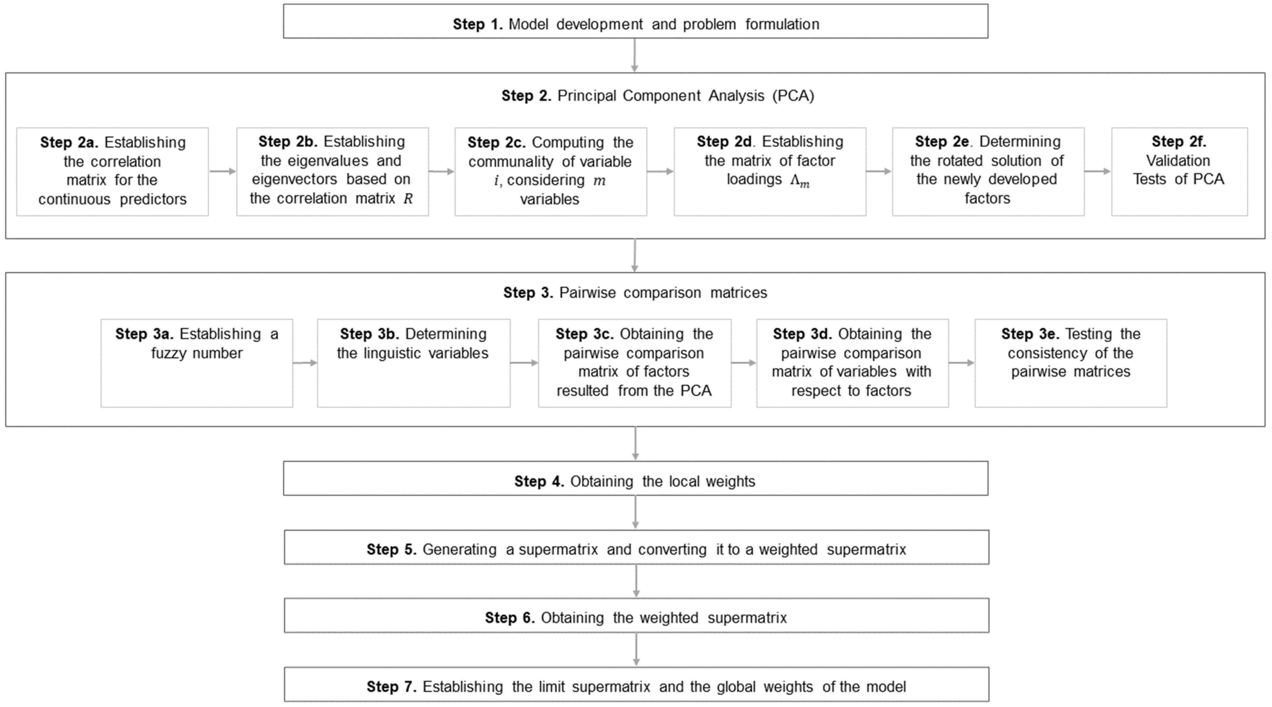
3.1. Proposed Method of Fuzzy-ANP with PCA

As previously mentioned, fuzzy-ANP depicts any decision-making problem as a network of elements arranged in clusters [49]. Nonetheless, general implementation of this method implies human judgements, which may lead to prejudiced outcomes. Moreover, due to the complexity of fuzzy-ANP, Ergu [46] emphasized the need to solve the issues with inconsistencies in the matrices. To solve these issues of biases and inconsistencies, this newly proposed methodology integrates an important and objective phase of principal component analysis. The PCA results are then integrated in the fuzzy-ANP framework. Although the methods of PCA [25,39] and fuzzy-ANP [53,54] are widely known and applied in terms of the evaluation of bank-related activities for decision selection, they have been investigated separately. General application of fuzzy-ANP involves collecting the primary data from decision making. In this newly proposed framework of using secondary data for fuzzy-ANP with PCA, this method aims to reduce the risk of information gaps and/or biases that may occur in methodologies relying exclusively on primary data. In this paper, we propose an innovative integration of these techniques for a multi-analytical fuzzy-ANP with PCA approach. For this newly established multi-analytic and unbiased methodology, the following steps are proposed (Figure 1):

• Step 1. Model development and problem formulation

This developing model aims to establish the relative importance weights of the variables proposed for evaluating a bank performance model under the assumption of country risk. Considering an innovative and multi-analytic dual-phase model, existing studies provided the foundation for variable selection, whereas the principal component analysis was applied to reduce the variables in every phase to a lower number of factors. The resulting PCA factors, together with the initial variables collected from the secondary data, represent the interconnected elements in a hierarchical network structure (Figure 2).

• Step 2. Principal Component Analysis (PCA)

Initially introduced by Pearson in 1901 [55], principal component analysis is applied when the main objective is to establish a minimum number of factors that aim to explain the highest level of variance observed in the data, with the intention to use these newly developed factors in subsequent analyses [56,57]. In other words, PCA generates new variables, i.e., principal components or factors, from “linear combinations of the original variables” [58]. As an interdependent procedure, PCA aims to “define the underlying structure among the variables in the analysis” [59]. Thus, PCA focuses on minimizing the information loss and adequately representing the original dataset [59,60]. Previous studies support the inclusion of PCA in country risk assessment and bank evaluation [25,31,39]. For PCA, the following steps are relevant for the analysis.

• Step 2a. Establishing the correlation matrix for the continuous predictors

Let X₁, X₂, …, X_m be m observed variables. The starting point of PCA involves the development of the correlation matrix R [61,62,63]:

$$R=\left[\begin{array}{cc}\begin{array}{cc}{r}_{11}& r_{12}\\ r_{21}& r_{21}\end{array}& \begin{array}{cc}\cdots & r_{1m}\\ \dots & r_{21}\end{array}\\ \begin{array}{cc}⋮& ⋮\\ r_{m1}& r_{m2}\end{array}& \begin{array}{cc}{r}_{ij}& ⋮\\ \dots & r_{mm}\end{array}\end{array}\right]$$

(1)

where

$$r_{ij}=\frac{{\sum }_{k=1}^n(X_{i_k}-\overline{X_i})(X_{j_k}-\overline{X_j})}{\sqrt{{\sum }_{k=1}^n{(X_{i_k}-\overline{X_i})}^2\times {\sum }_{k=1}^n{(X_{j_k}-\overline{X_j})}^2}}$$

(2)

• Step 2b. Establishing the eigenvalues and eigenvectors based on the correlation matrix R

For the next step, we compute λ₁ ≥ λ₂ ≥…≥ λ_m as the eigenvalues (sorted in descending order) and ω₁, ω₂,…, ω_m as their corresponding eigenvectors of R. The eigenvalues are calculated based on the following [64]:

$$\left|R-\lambda I\right|=0$$

(3)

The corresponding eigenvectors of R are computed as follows:

$$\left(R-{\lambda }_{i}I\right){\omega }_j=0$$

(4)

• Step 2c. Computing the communality of variable i, considering m variables

For PCA, a communality represents the “estimate of its shared, or common, variance among the variables as represented by the derived factors” [59], calculated as follows [61,65]:

$$h_i=\sum _{j=1}^m\left|{\lambda }_j\right|{\omega }_{ij}^2$$

(5)

For each variable included in the PCA, the communality should adhere to a recommended threshold of 0.5 [59].

• Step 2d. Establishing the matrix of factor loadings ${\Lambda }_m$ considering the following equation [61,65]:

$${\Lambda }_m={\mathsf{\Omega }}_m{\mathsf{\Gamma }}_m^{1/2}$$

(6)

where

${\mathsf{\Omega }}_m=({\omega }_1,{\omega }_2,\dots ,{\omega }_m)$, ${\mathsf{\Gamma }}_m=diag(\left|{\lambda }_1\right|,\left|{\lambda }_2\right|,\dots ,\left|{\lambda }_m\right|)$

Factor loadings reflect the correlation between the examined variables and the developed factor [59,65]. To establish the number of relevant extracted factors, previous studies have recommended retaining all of the factors that have eigenvalues greater than 0.7 [64], while considering the percentage of variance criterion of a 60% suggested threshold [59]. Thus, by applying principal component analysis in IBM SPSS Statistics v.26 (IBM Corp., Armonk, NY, USA), we obtained the following component matrix, corresponding to Equation (6):

$$\Lambda =\left[\begin{array}{ccc}{\lambda }_{11}^{1/2}& \dots & {\lambda }_{1n}^{1/2}\\ ⋮& {\lambda }_{i\mathcal{l}}^{1/2}& ⋮\\ {\lambda }_{m1}^{1/2}& \dots & {\lambda }_{mn}^{1/2}\end{array}\right]$$

(7)

where Eigenvalue ${\lambda }_{\mathcal{l}}$ > 0.7 [64] associated with factor $\mathcal{l}$ is

$${\lambda }_{\mathcal{l}}=\sum _{i=1}^m{\lambda }_{i\mathcal{l}}^{1/2}$$

(8)

and communality $h_i$, based on corresponding Equation (5), can be expressed by

$$h_i=\sum _{\mathcal{l}=1}^m{\lambda }_{i\mathcal{l}}^{1/2},where h_i>0.5$$

(9)

• Step 2e. Determining the rotated solution of the newly developed factors

After establishing and retaining the number of principal components based on recommended frameworks, the next step in PCA involves the rotation. The rotated solutions of the factor matrix reflect a more meaningful and significant factor pattern, which is achieved by redistributing the variance from earlier components to subsequent ones [59]. Varimax rotation is recommended [58,65] as it “maximizes the sum of variances of required loadings of the factor matrix” [66]. Factor matrix is normalized by the square root of communalities [58,61,64,65], considering:

$${\Lambda }_m^{\mathrm{*}}=H^{-1/2}{\Lambda }_m$$

(10)

where

${\Lambda }_m=({\underset{\_}{\lambda }}_1,{\underset{\_}{\lambda }}_2,\dots ,{\underset{\_}{\lambda }}_m)$ is the factor pattern matrix;

$H=diag(h_1,h_2,\dots ,h_n)$ is the diagonal matrix of communalities.

Varimax generates i iterations by searching for linear combinations, until the variance of the square loadings is maximized:

$${SV}_{\left(i\right)}=\sum _{j=1}^m\left(n\sum _{k=1}^n{{\lambda }_{kj\left(i\right)}^{*}}^4-{\left(\sum _{k=1}^n{{\lambda }_{kj\left(i\right)}^{*}}^2\right)}^2\right)/n^2$$

(11)

where the initial ${\Lambda }_{m\left(1\right)}^{\mathrm{*}}$ indicates the original factor pattern matrix. Considering successive iterations, the primary value represents the final value of ${\Lambda }_{m(i-1)}^{\mathrm{*}}$, once factor pairs showcase rotation [61].

After rotation, we rearrange the rotated factors so that [61]

$$\sum _{i=1}^m{\widetilde{{\lambda }_{i1}}}^2\ge \dots \ge \sum _{i=1}^m{\widetilde{{\lambda }_{in}}}^2$$

(12)

Based on Equations (10)–(12), we have the following rotated matrix with n rotated factors and m variables:

$${\tilde{\mathsf{\Lambda }}}_{m\times n}=\left[\begin{array}{c}\begin{array}{ccc}\widetilde{{\lambda }_{11}}& \dots & \widetilde{{\lambda }_{1n}}\\ \widetilde{{\lambda }_{21}}& \dots & \widetilde{{\lambda }_{2n}}\\ ⋮& \widetilde{{\lambda }_{i\mathcal{l}}}& ⋮\end{array}\\ \begin{array}{ccc}\widetilde{{\lambda }_{m1}}& \dots & \widetilde{{\lambda }_{mn}}\end{array}\end{array}\right]$$

(13)

From this matrix, the following n factors are obtained:

$$f_{\mathcal{l}}=\sum _{i=1}^m{\widetilde{{\lambda }_{i\mathcal{l}}}}^2=\sum _{i=1}^m{v}_{{\mathcal{l}}_i}$$

(14)

Derived from Equation (14), we have variable $v_{{\mathcal{l}}_i}$ with respect to every factor $f_{\mathcal{l}}$ determined by the following expression:

$$v_{{\mathcal{l}}_i}={\widetilde{{\lambda }_{i\mathcal{l}}}}^2$$

(15)

As the results of PCA, all factors $f_{\mathcal{l}}$ and variables $v_{{\mathcal{l}}_i}$ are integrated into fuzzy-ANP to construct pairwise comparison matrices.

• Step 2f. Validation Tests of PCA

Before proceeding to the next phase of the fuzzy-ANP, the accuracy of PCA needs to be assessed based on relevancy tests. First, Chi-square value for Bartlett’s test of sphericity (and its associated significance test) tests the presence of relevant correlations for the set of examined variables [59,61,62,65,66]:

$${\chi }^2=-\left(W-1-\frac{2p+5}{6}\right)log\left|C\right|$$

(16)

with p(p − 1)/2 degrees of freedom.

Second, Kaiser–Mayer–Olkin measure of sample adequacy identifies the appropriateness of the solution, based on values higher than 0.7 [61,67,68]:

$${KMO}_j=\frac{{\sum }_{i\ne j}{r}_{ij}^2}{{\sum }_{i\ne j}{r}_{ij}^2+{\sum }_{i\ne j}{a}_{ij}^{2*}}$$

(17)

$$KMO=\frac{{\sum }_{i\ne j}\sum r_{ij}^2}{{\sum }_{i\ne j}\sum r_{ij}^2+\sum _{i\ne j}\sum a_{ij}^{2*}}$$

(18)

where $a_{ij}^{*}$ is the anti-image correlation coefficient.

• Step 3. Pairwise comparison matrices

After validating the PCA, we proceed to the fuzzy-ANP phase. As a widely popular technique [41,47,48], fuzzy-ANP has shown versatility in a broad spectrum of contexts. For the fuzzy-ANP method, first, we define a fuzzy number and corresponding linguistic variables.

• Step 3a. Establishing a fuzzy number

At this phase in the mathematical technique, a fuzzy number [69] is established:

$$\widetilde{A_i^{*}}=\left\{\begin{array}{c}(x_i-l_i)/(m_i-l_i),\\ (u_i-x_i)/(u_i-m_i), \\ 0,\end{array} \right. \begin{array}{c} l_i\le x_i\le m_i\\ m_i\le x_i\le u_i\\ otherwise\end{array}$$

(19)

In Equation (19), $l_i$ and $u_i$ reflect the lower and upper bounds for the fuzzy number $\widetilde{A_i^{\mathrm{*}}}$, and $m_i$ indicates the modal value for $\widetilde{A_i^{\mathrm{*}}}$. The triangular fuzzy number (TFN0) [70,71], is expressed as follows

$$\widetilde{A_i^{\mathrm{*}}}=\left(l_i,m_i,u_i\right)$$

(20)

while the reciprocal of the fuzzy number is as follows:

$${\widetilde{A_i^{\mathrm{*}}}}^{-1}={(l_i,m_i,u_i)}^{-1}=(1/u_i,1/m_i,1/l_i)$$

(21)

• Step 3b. Determining the linguistic variables

The relative importance of the elements is measured based on Saaty’s nine-point scale [42,43,72,73,74]. This scale is further transformed to a fuzzy triangular scale, according to

Table 1. Linguistic terms and their corresponding triangular fuzzy numbers [28].

Saaty’s Scale	Linguistic Terms	Fuzzy Triangular Scale
9	Extremely importance	(9, 9, 9)
8	Very, very strong	(7, 8, 9)
7	Very strong importance	(6, 7, 8)
6	Strong plus	(5, 6, 7)
5	Strong importance	(4, 5, 6)
4	Moderate plus	(3, 4, 5)
3	Moderate importance	(2, 3, 4)
2	Weak	(1, 2, 3)
1	Equal importance	(1, 1, 1)

.

• Step 3c. Obtaining the pairwise comparison matrix of factors resulted from the PCA

Let f₁, f₂, …, f_n be n factors resulting from PCA, sorted in descending order, f₁ ≥ f₂ ≥ … ≥ f_n. To transform the data for pairwise comparison based on Saaty’s scale [28,43], the following min–max normalization formula is applied [74,75,76]:

$$f_{\mathcal{l}}^{\mathrm{*}}=\frac{f_{\mathcal{l}}-{min}_F}{{max}_F-{min}_F}\left({new\_max}_F-{new\_min}_F\right)+{new\_min}_F$$

(22)

where

$$\begin{gathered} {max}_F=\mathrm{m}\mathrm{a}\mathrm{x}(f_1,f_2,\dots ,f_n) \\ {min}_F=\mathrm{m}\mathrm{i}\mathrm{n}(f_1,f_2,\dots ,f_n) \\ {new\_max}_F=9 \\ {new\_min}_F=1 \end{gathered}$$

(23)

Following this step, we obtain values $f_{ij}^{*}$ that are assigned to fuzzy number $\widetilde{f_{ij}^{*}}$.

$$\begin{array}{c}{f}_{ij}^{\mathrm{*}}=\frac{f_i^{\mathrm{*}}}{f_j^{\mathrm{*}}}\\ f_{ji}^{\mathrm{*}}=\frac{1}{f_{ij}^{\mathrm{*}}}\end{array},where f_i^{\mathrm{*}}\ge f_j^{\mathrm{*}}$$

(24)

Linguistic terms to the pairwise comparisons are assigned by using Equations (19)–(24), and based on Table 1, the resulting fuzzy pairwise comparison matrix $\tilde{F}$ is developed:

$$\tilde{F}=\left[\begin{array}{cc}\begin{array}{cc}\begin{array}{c}\begin{array}{c}1\\ 1/\widetilde{f_{21}^{\mathrm{*}}}\end{array}\\ \begin{array}{c}⋮\\ 1/\widetilde{f_{1n}^{\mathrm{*}}}\end{array}\end{array}& \begin{array}{c}\begin{array}{c}\widetilde{f_{12}^{\mathrm{*}}}\\ 1\end{array}\\ \begin{array}{c}⋮\\ 1/\widetilde{f_{2n}^{\mathrm{*}}}\end{array}\end{array}\end{array}& \begin{array}{cc}\begin{array}{c}\begin{array}{c}\cdots \\ \cdots \end{array}\\ \begin{array}{c}\ddots \\ \dots \end{array}\end{array}& \begin{array}{c}\begin{array}{c}\widetilde{f_{1n}^{\mathrm{*}}}\\ \widetilde{f_{2n}^{\mathrm{*}}}\end{array}\\ \begin{array}{c}⋮\\ 1\end{array}\end{array}\end{array}\end{array}\right]$$

(25)

Step 3d. Obtaining the pairwise comparison matrix of variables with respect to factors

Let $v_{{\mathcal{l}}_1},v_{{\mathcal{l}}_2},\dots ,v_{{\mathcal{l}}_n}$ be m variables with respect to factor $f_{\mathcal{l}}$ resulting from PCA. We use the following min–max normalization formula [74,75,76] to transform the data:

$$v_{{\mathcal{l}}_i}^{*}=\frac{v_{{\mathcal{l}}_i}-{min}_{V_{\mathcal{l}}}}{{max}_{V_{\mathcal{l}}}-{min}_{V_{\mathcal{l}}}}\left({new\_max}_{V_{\mathcal{l}}}-{new\_min}_{V_{\mathcal{l}}}\right)+{new\_min}_{V_{\mathcal{l}}}$$

(26)

where

$$\begin{gathered} {max}_{V_{\mathcal{l}}}=\mathrm{m}\mathrm{a}\mathrm{x}\left(v_{{\mathcal{l}}_1},v_{{\mathcal{l}}_2},\dots ,v_{{\mathcal{l}}_3}\right) \\ {min}_{V_{\mathcal{l}}}=\mathrm{m}\mathrm{i}\mathrm{n}\left(v_{{\mathcal{l}}_1},v_{{\mathcal{l}}_2},\dots ,v_{{\mathcal{l}}_3}\right) \\ {new\_max}_{V_{\mathcal{l}}}=9 \\ {new\_min}_{V_{\mathcal{l}}}=1 \end{gathered}$$

(27)

Following this, we obtain values $v_{c_{ij}}^{*}$ that are assigned to fuzzy number $\widetilde{v_{c_{ij}}^{*}}$.

$$\begin{array}{c}{v}_{{\mathcal{l}}_{ij}}^{*}=\frac{v_{{\mathcal{l}}_i}^{*}}{v_{{\mathcal{l}}_j}^{*}}\\ v_{{\mathcal{l}}_{ji}}^{*}=\frac{1}{v_{{\mathcal{l}}_{ij}}^{*}}\end{array}, where v_{{\mathcal{l}}_i}^{*}\ge v_{{\mathcal{l}}_j}^{*}$$

(28)

Fuzzy pairwise comparison matrix $\widetilde{V_{\mathcal{l}}}$ is constructed in the same manner as the matrix from Step 3c.

$$\widetilde{V_{\mathcal{l}}}=\left[\begin{array}{cc}\begin{array}{cc}1& \stackrel{~}{v_{{\mathcal{l}}_{12}}^{*}}\\ 1/\stackrel{~}{v_{{\mathcal{l}}_{12}}^{*}}& 1\end{array}& \begin{array}{cc}\dots & \stackrel{~}{v_{{\mathcal{l}}_{1n}}^{*}}\\ \dots & \stackrel{~}{v_{{\mathcal{l}}_{2n}}^{*}}\end{array}\\ \begin{array}{cc}⋮& ⋮\\ 1/\stackrel{~}{v_{{\mathcal{l}}_{1n}}^{*}}& 1/\stackrel{~}{v_{{\mathcal{l}}_{2n}}^{*}}\end{array}& \begin{array}{cc}\ddots & ⋮\\ \dots & 1\end{array}\end{array}\right]$$

(29)

• Step 3e. Testing the consistency of the pairwise matrices

The most well-known consistency test [46,77] for the pairwise comparison matrices in ANP is the consistency ratio by Saaty [28,43]:

$$CR=\frac{{\lambda }_{max}-n}{(n-1)RI}$$

(30)

where λ_max is the maximum eigenvalue of a matrix, n is the order of the matrix, and RI is the average random matrix index proposed by Saaty [28,43]. The comparison matrix is consistent if the value of CR is less than 0.1 [28,41,43,46,77]. By integrating PCA, consistency is assured for the matrices obtained in the preceding steps associated with fuzzy-ANP.

• Step 4. Obtaining the local weights

Let $X=\{x_1,x_2,\dots ,x_{\mathcal{t}}\}$ be an object and $U=\{u_1,u_2,\dots ,u_{\mathcal{p}}\}$ be the goal set. As stated by Chang’s extent analysis method [69], each object is considered, and extent analysis is applied for each goal $u_i$. Then, for each $\mathcal{p}$ from Chang’s extent analysis, each object can be expressed by $M_{g_i}^1,M_{g_i}^2,\dots ,M_{g_i}^{\mathcal{p}}$, $i=1,2,\dots ,\mathcal{t}$, where all of the $M_{g_i}^j(j=1, 2, \dots ,\mathcal{p})$ represent TFNs.

First, the value of fuzzy synthetic extent with respect to i-th object is as follows [69]:

$$S_i=\sum _{j=1}^{\mathcal{p}}{M}_{g_i}^j\otimes {\left[\sum _{i=1}^{\mathcal{t}}\sum _{j=1}^{\mathcal{p}}{M}_{g_i}^j\right]}^{-1}$$

(31)

where

$$\sum _{j=1}^{\mathcal{p}}{M}_{g_i}^j=\left(\sum _{j=1}^{\mathcal{p}}{l}_j,\sum _{j=1}^{\mathcal{p}}{m}_j,\sum _{j=1}^{\mathcal{p}}{u}_j\right)$$

(32)

$${\left[\sum _{i=1}^{\mathcal{t}}\sum _{j=1}^{\mathcal{p}}{M}_{g_i}^j\right]}^{-1}=\left(\frac{1}{{\sum }_{i=1}^{\mathcal{t}}{\sum }_{j=1}^{\mathcal{p}}{u}_{ij}},\frac{1}{{\sum }_{i=1}^{\mathcal{t}}{\sum }_{j=1}^{\mathcal{p}}{m}_{ij}},\frac{1}{{\sum }_{i=1}^{\mathcal{t}}{\sum }_{j=1}^{\mathcal{p}}{l}_{ij}}\right)$$

(33)

Hence,

$$S_i=\left(\sum _{j=1}^{\mathcal{p}}{l}_j,\sum _{j=1}^{\mathcal{p}}{m}_j,\sum _{j=1}^{\mathcal{p}}{u}_j\right)\otimes \left(\frac{1}{{\sum }_{i=1}^{\mathcal{t}}{\sum }_{j=1}^{\mathcal{p}}{u}_{ij}},\frac{1}{{\sum }_{i=1}^{\mathcal{t}}{\sum }_{j=1}^{\mathcal{p}}{m}_{ij}}, \frac{1}{{\sum }_{i=1}^{\mathcal{t}}{\sum }_{j=1}^{\mathcal{p}}{l}_{ij}}\right)$$

(34)

Second, the degree possibility $S_2=(l_2,m_2,u_2)\ge S_1=(l_1,m_1,u_1)$ is expressed as follows [48,69,78]:

$$V\left(S_2\ge S_1\right)=sup\left[\mathrm{m}\mathrm{i}\mathrm{n}({\mu }_{S_1}\left(x\right),{\mu }_{S_2}\left(y\right))\right]=\left\{\begin{array}{c}1, if m_2\ge m_1\\ 0, if l_1\ge l_2\\ \frac{l_1-u_2}{\left(m_2-u_2\right)-(m_1-l_1)}\end{array}\right.$$

(35)

According to Chang [69]: “the degree possibility for a convex fuzzy number to be greater than k convex fuzzy numbers $S_i(i=1,2,\dots ,k)$”, is defined by the following [69]:

$$\begin{gathered} V\left(S\ge S_1,S_2,\dots ,S_k\right) \\ =V\left[\left(S\ge S_1\right) and \left(S\ge S_2\right) and \dots and \left(S\ge S_k\right)\right] \\ =minV\left(S\ge S_i\right), i=1, 2, \dots , k \end{gathered}$$

(36)

Assuming that

$$d^{\prime }\left(A_i\right)=minV\left(S_i\ge S_k\right), for k=1, 2,\dots ,n;k\ne i.$$

(37)

we obtain the following weight vector:

$$W^{\prime }={\left(d^{\prime }\left(A_1\right),d^{\prime }\left(A_2\right),\dots ,d^{\prime }\left(A_{\mathcal{t}}\right)\right)}^T, where A_i\left(i=1,2,\dots ,\mathcal{t}\right) are \mathcal{t} elements.$$

(38)

Through normalization, we find the normalized weight vectors:

$$W_i={\left(d\left(A_1\right),d\left(A_2\right),\dots ,d\left(A_{\mathcal{t}}\right)\right)}^T$$

(39)

where $W_i$ indicates a nonfuzzy number.

• Step 5. Generating a supermatrix and converting it to a weighted supermatrix

A supermatrix illustrates the impact of a network’s distinct elements on the other elements in the same network [41]. The columns of the supermatrix are populated with the weights obtained from previous steps [28]. To attain overall priorities in a system’s interaction, internal importance vectors are included into columns, based on the connection between elements [72]. In this model, the supermatrix representation is provided as follows [47,79]:

$$W=\left[\begin{array}{ccc}0& 0& 0\\ W_{21}& 0& 0\\ 0& W_{32}& I\end{array}\right]$$

(40)

The vector of $W_{21}$ represents the local weights vector of the factors with respect to the goal, the vector of $W_{32}$ represents the local weights vector of the variables with respect to each factor, and $I$ represents the identity matrix [47].

• Step 6. Obtaining the weighted supermatrix

To obtain the weighted supermatrix, entries of the initial supermatrix are divided by the sum of the weights of their corresponding column. The following weighted supermatrix is obtained [44]:

$$W_n=\left[\begin{array}{ccc}\frac{W_{11}}{d_1}& \dots & \frac{W_{1n}}{d_n}\\ ⋮& \ddots & ⋮\\ \frac{W_{n1}}{d_1}& \dots & \frac{W_{nn}}{d_n}\end{array}\right]$$

(41)

where

$$d_j=\sum _{j=1}^n{W}_{ij}$$

(42)

• Step 7. Establishing the limit supermatrix and the global weights of the model

The limit supermatrix is computed by multiplying the weighted supermatrix by itself until the values are stabilized [28,44].

$$L=\underset{g\to \mathrm{\infty }}{\lim }{\left(W_n^{\propto }\right)}^g$$

(43)

The limit supermatrix yields the relative importance weights for each variable included in the model. [28].

3.2. Method for Country Risk Assessment

The fuzzy-ANP with PCA method proposed in Section 3.1. is adapted for a country risk assessment model. To establish this model, this empirical analysis involved data collection and variable explanations from Refinitiv Thomson Reuters, considering a set of 172 countries with complete data for the variables considered. A set of 17 variables were selected based on previous examinations [1,4,20,25,27,30,36,39]. The collected data followed the measurement scale proposed by Refinitiv, ranging from 1 (very low risk) to 5 (very high risk). This model assessed a 2016–2022 timeframe, for a total of 1204 observations. Further details on these variables are presented in

Table 2. Country risk variables.

Environment		Variable	Variable Description	Mean	SD
Political environment	X1	Type of governance	Progress and transformation process towards democracy and market economy	2.7749	1.0648
	X2	Civil liberties & political rights	Freedom of individuals in terms of individual rights and personal autonomy, and government functioning along with electoral and political participation	2.8978	1.1917
	X3	Freedom of the press	Journalistic freedom and free flow of news	2.9111	1.0568
	X4	Political stability	Likelihood of political destabilization and interferences in governmental jurisdiction	2.9045	0.9760
	X5	Regulatory quality	Sound policies to support private sector activity	2.9668	0.9583
	X6	Rule of law	Aggregated individual governance indicators of economies	3.0291	0.9836
	X7	Armed conflict	Potential conflict based on clashing interests	2.9203	0.9880
	X8	Human rights	State respect regarding human rights indicators	2.9543	1.0333
	X9	Voice & accountability	Perceptions of citizens’ freedom of expression and association	2.9668	1.0414
Economic environment	X10	Average earnings	Economy classification based on Gross National Income per capita	3.0739	1.1713
	X11	Economic freedom	Benchmarks highlighting freedom of trade, business, investment, etc.	2.9344	1.0168
	X12	Sovereign credit ratings	Risk level of debt that is guaranteed by the sovereign	3.0033	0.9181
	X13	Competitiveness	Economic classification based on the Global Competitiveness Index	3.0008	1.0351
Criminal environment	X14	Corruption	Abuse level of power for personal gain	2.9236	1.0495
	X15	Natural resources industry controls	Assessment of industry controls in resource-rich countries	2.8887	1.1694
	X16	Terrorism	Assessment of country terrorism fatalities and threats	2.9618	0.8074
	X17	Absence of violence	Assessment of ‘peace’ level based on internal and external conflicts	2.8912	0.9738

.

The fuzzy-ANP with PCA provides the mathematical framework for this proposed model’s country risk assessment. Conceptually, in this paper, the country risk model is described as a system of 17 dimensions (variables) that interact with each dimension with respect to n factors obtained with PCA. The fuzzy-ANP with PCA provides a multicriteria model of country risk assessment based on the steps presented in Section 3.1. This section provides the basis for model validation in Section 4.1.

3.2.1. Extracting Country Risk Factors with PCA

To start, we apply the PCA mathematical technique for variables $X_1,X_2,\dots ,X_{17}$ (Table 2). Following Steps 2a–f and applying the algorithm based on Equations (1)–(18), the analysis extracts n factors. In the following step, the 17 variables $X_i$ are pairwise compared with respect to each factor $f_{\mathcal{l}}$.

3.2.2. Constructing Pairwise Comparison Matrices for Factors and Variables: Obtaining the Local Weights for the Country Risk Model

From PCA, we obtain factors $f_1,f_2,\dots ,f_n$, with each factor $f_{\mathcal{l}}$ corresponding to variables $v_{{\mathcal{l}}_1},v_{{\mathcal{l}}_2},\dots ,v_{{\mathcal{l}}_{17}}$. Based on the previously mentioned Steps 3a–3e and Equations (19)–(30), pairwise comparison matrices for the factors and their associated variables are obtained.

Considering Chang’s [69] extent analysis (Step 4), we apply Equations (31)–(39). Based on this process, the normalized weight vectors are obtained. These vectors showcase the local weights for the country risk model.

3.2.3. Determining the Unweighted Supermatrix and Converting It to a Weighted Supermatrix

The weights obtained in previous steps are used to construct the unweighted supermatrix, based on Step 5. This matrix is normalized by applying Equation (42) to obtain the weighted supermatrix (Step 6).

3.2.4. Establishing the Limit Supermatrix and the Global Weights for the Country Risk Model

By applying Equation (43), the weighted supermatrix of the country risk model’s variables is multiplied by itself and the limit supermatrix is generated. This aspect provides the basis for extraction from the limit supermatrix of the global weights $w_1,w_2,\dots ,w_{17}$ associated with the country risk model’s variables. Thus, based on weights $w_i$, we obtain the country risk score ($R_k$ score), for each country k from the 172 considered countries, by applying the following formula:

$$R_k=\sum _{i=1}^{17}{w}_i{X}_{ik}$$

(44)

3.3. Method for Bank Performance Model under the Assumption of Country Risk

In this section, the fuzzy-ANP with PCA method proposed in Section 3.1. is adapted for the bank performance model. The country risk assessment results (namely, country risk scores $R_1, R_2,\dots ,R_{172}$) were further integrated in the next phase of this model to establish a bank performance evaluation model. For this proposed model, the data analysis included previously established country risk scores (based on fuzzy-ANP with PCA) and a set of bank-related variables collected from Refinitiv Thomson Reuters and International Monetary Fund (IMF) (Table 3). The data collection process involved filtering the set by public and listed companies, with the available data on the selected set of variables, for the timeframe of 2016–2022. For the bank performance assessment, this study included a set of commonly used indicators selected from the banking literature [1,20,27,30]. The final sample comprised 496 banks operating across 58 countries. Compared with the previous study of 172 countries for country risk assessment, this bank performance model retained a set of 58 countries based on bank-related data availability.

To examine bank performance, we opted for a straightforward approach. Two sets of variables were taken into account as the model’s explanatory variables. Firstly, we established a set of variables relative to the bank’s characteristics, based on previous research. Consistent with prior research [27,80,81], this study focused on return-on-assets (ROA) as the primary variable to illustrate bank performance. Following previous investigations [27,82], variables related to the financial profile of banks were considered, such as asset quality (AQ), earnings and profitability (E&P), capitalization and leverage (C&L), and funding and liquidity (F&L). Moreover, using direction from previous empirical studies [27,83,84], this analysis included other variables that showcased the characteristics of banks, namely ratio of equity to total assets (EQUITY) and bank size using the logarithm of total assets [SIZE]. Secondly, to reflect the impacts connected to economic conditions, two frequently applied indicators from banking investigations were selected, i.e., a country’s growth rate (GDP) and inflation rate (INF) [1,27,39]. Table 3 addresses the bank-specific variables used in this research.

Table 3. Variables of bank performance model under the assumption of country risk.

${\mathit{U}}_{{\mathit{v}}_{\mathit{\beta }}}|{\mathit{U}}_{{\mathit{v}}_{\mathit{k}}}$	${\mathit{v}}_{\mathit{\beta }}^{\mathbf{*}}$	${\mathit{m}\mathit{a}\mathit{x}}_{\mathit{v}}$	${\mathit{m}\mathit{i}\mathit{n}}_{\mathit{v}}$	${\mathit{v}}_{\mathit{\beta }}$	Description	Mean	SD
$U_{{ROA}_{\beta }}={ROA}_{\beta }^{*}{e}^{-R_k}$	${ROA}_{\beta }^{\mathrm{*}}=\frac{{ROA}_{\beta }-7.83}{7.83-(-0.12)}$	7.83 b	−0.12 b	ROA	Ratio of net profit to total assets (%, 4-year average)	1.12	0.62
$U_{{AQ}_{\beta }}={AQ}_{\beta }^{*}{e}^{-R_k}$	${AQ}_{\beta }^{\mathrm{*}}=1-\frac{{AQ}_{\beta }-0.25}{14-0.25}$	14 a	0.25 a	AQ	Ratio of impaired loans to gross loans (%, 4-year average)	2.17	3.34
$U_{{E\&P}_{\beta }}={E\&P}_{\beta }^{*}{e}^{-R_k}$	${E\&P}_{\beta }^{\mathrm{*}}=\frac{{E\&P}_{\beta }-(-0.25)}{5-(-0.25)}$	5 a	−0.25 a	E&P	Ratio of operating profit to risk-weighted assets (%, 4-year average)	4.14	36.78
$U_{{C\&L}_{\beta }}={C\&L}_{\beta }^{*}{e}^{-R_k}$	${C\&L}_{\beta }^{\mathrm{*}}=\frac{{C\&L}_{\beta }-6}{22-6}$	22 a	6 a	C&L	Core capital ratio (%)	15.09	4.54
$U_{{F\&L}_{\beta }}={F\&L}_{\beta }^{*}{e}^{-R_k}$	${F\&L}_{\beta }^{\mathrm{*}}=1-\frac{{F\&L}_{\beta }-45}{250-45}$	250 a	45 a	F&L	Ratio of loans to customer deposits (%, 4-year average)	109.20	63.12
$U_{{SIZE}_{\beta }}={SIZE}_{\beta }^{*}{e}^{-R_k}$	${SIZE}_{\beta }^{\mathrm{*}}=\frac{{SIZE}_{\beta }-18.94}{19.14-18.94}$	29.14 b	18.94 b	SIZE	Natural logarithm of total assets (%, 4-year average)	23.19	1.98
$U_{{EQUITY}_{\beta }}={EQUITY}_{\beta }^{*}{e}^{-R_k}$	${EQUITY}_{\beta }^{\mathrm{*}}=\frac{{EQUITY}_{\beta }-2.46}{46.65-2.46}$	46.65 b	2.46 b	EQUITY	Ratio of equity to total assets (%, 4-year average)	10.71	3.39
$U_{{GDP}_k}={GDP}_k^{*}{e}^{-R_k}$	${GDP}_k^{\mathrm{*}}=\frac{{GDP}_k-13.55}{13.55-(-15.70)}$	13.55 b	−15.70 b	GDP	GDP growth rate of the country (%)	2.07	3.89
$U_{{INF}_k}={INF}_k^{*}{e}^{-R_k}$	${INF}_k^{\mathrm{*}}=1-\frac{{INF}_k-2}{64.27-2}$	64.27 b	2	INF	Inflation rate of the country (%)	4.66	5.96

Note: ^a minimum and maximum levels are provided in accordance with the Fitch Rating methodology for rating banks [82]; ^b minimum and maximum of the values set.

Table 3. Variables of bank performance model under the assumption of country risk.

${\mathit{U}}_{{\mathit{v}}_{\mathit{\beta }}}|{\mathit{U}}_{{\mathit{v}}_{\mathit{k}}}$	${\mathit{v}}_{\mathit{\beta }}^{\mathbf{*}}$	${\mathit{m}\mathit{a}\mathit{x}}_{\mathit{v}}$	${\mathit{m}\mathit{i}\mathit{n}}_{\mathit{v}}$	${\mathit{v}}_{\mathit{\beta }}$	Description	Mean	SD
$U_{{ROA}_{\beta }}={ROA}_{\beta }^{*}{e}^{-R_k}$	${ROA}_{\beta }^{\mathrm{*}}=\frac{{ROA}_{\beta }-7.83}{7.83-(-0.12)}$	7.83 b	−0.12 b	ROA	Ratio of net profit to total assets (%, 4-year average)	1.12	0.62
$U_{{AQ}_{\beta }}={AQ}_{\beta }^{*}{e}^{-R_k}$	${AQ}_{\beta }^{\mathrm{*}}=1-\frac{{AQ}_{\beta }-0.25}{14-0.25}$	14 a	0.25 a	AQ	Ratio of impaired loans to gross loans (%, 4-year average)	2.17	3.34
$U_{{E\&P}_{\beta }}={E\&P}_{\beta }^{*}{e}^{-R_k}$	${E\&P}_{\beta }^{\mathrm{*}}=\frac{{E\&P}_{\beta }-(-0.25)}{5-(-0.25)}$	5 a	−0.25 a	E&P	Ratio of operating profit to risk-weighted assets (%, 4-year average)	4.14	36.78
$U_{{C\&L}_{\beta }}={C\&L}_{\beta }^{*}{e}^{-R_k}$	${C\&L}_{\beta }^{\mathrm{*}}=\frac{{C\&L}_{\beta }-6}{22-6}$	22 a	6 a	C&L	Core capital ratio (%)	15.09	4.54
$U_{{F\&L}_{\beta }}={F\&L}_{\beta }^{*}{e}^{-R_k}$	${F\&L}_{\beta }^{\mathrm{*}}=1-\frac{{F\&L}_{\beta }-45}{250-45}$	250 a	45 a	F&L	Ratio of loans to customer deposits (%, 4-year average)	109.20	63.12
$U_{{SIZE}_{\beta }}={SIZE}_{\beta }^{*}{e}^{-R_k}$	${SIZE}_{\beta }^{\mathrm{*}}=\frac{{SIZE}_{\beta }-18.94}{19.14-18.94}$	29.14 b	18.94 b	SIZE	Natural logarithm of total assets (%, 4-year average)	23.19	1.98
$U_{{EQUITY}_{\beta }}={EQUITY}_{\beta }^{*}{e}^{-R_k}$	${EQUITY}_{\beta }^{\mathrm{*}}=\frac{{EQUITY}_{\beta }-2.46}{46.65-2.46}$	46.65 b	2.46 b	EQUITY	Ratio of equity to total assets (%, 4-year average)	10.71	3.39
$U_{{GDP}_k}={GDP}_k^{*}{e}^{-R_k}$	${GDP}_k^{\mathrm{*}}=\frac{{GDP}_k-13.55}{13.55-(-15.70)}$	13.55 b	−15.70 b	GDP	GDP growth rate of the country (%)	2.07	3.89
$U_{{INF}_k}={INF}_k^{*}{e}^{-R_k}$	${INF}_k^{\mathrm{*}}=1-\frac{{INF}_k-2}{64.27-2}$	64.27 b	2	INF	Inflation rate of the country (%)	4.66	5.96

Note: ^a minimum and maximum levels are provided in accordance with the Fitch Rating methodology for rating banks [82]; ^b minimum and maximum of the values set.

Considering the existing framework [74,75,76], data were preprocessed and standardized for analysis by applying the min–max normalization formula [74,75,76] for every variable in Table 3:

$$v_{\beta }^{\mathrm{*}}=\frac{v_{\beta }-{min}_v}{{max}_v-{min}_v} normalized by maximizing$$

(45)

$$v_{\beta }^{\mathrm{*}}=1-\frac{v_{\beta }-{min}_v}{{max}_v-{min}_v} normalized by minimazing$$

(46)

where $v_{\beta }$ refers to variable $v$ of bank $\beta$.

To evaluate bank performance, we determined a model under the assumption of country risk based on the following utility functions:

$$U_{v_{\beta }}=v_{\beta }{e}^{-R_k}, for banking variables$$

(47)

$$U_{v_k}=v_k{e}^{-R_k}, for country variables$$

(48)

The fuzzy-ANP with PCA provides a multicriteria model of bank performance under the assumption of country risk based on the steps presented in Section 3.1. This section provides the basis for model validation in Section 4.2.

3.3.1. Extracting Bank Performance Factors with PCA

To begin with, we applied PCA for variables $U_{{ROA}_{\beta }},U_{{AQ}_{\beta }},U_{{E\&P}_{\beta }},U_{{C\&L}_{\beta }},U_{{F\&L}_{\beta }},U_{{EQUITY}_{\beta }},U_{{SIZE}_{\beta }},U_{{GDP}_k},U_{{INF}_k}$ (Table 3). Following Steps 2a–e and the algorithm reflected in Equations (1)–(15), the analysis showed n number of factors. In the following step, the nine variables were pairwise compared with respect to each factor $f_{\mathcal{l}}$.

3.3.2. Constructing the Pairwise Comparison Matrices for Factors and Variables: Obtaining Local Weights for the Bank Performance Model under the Assumption of Country Risk

Factors $f_1,f_2,\dots ,f_n$ result from PCA, and each factor $f_{\mathcal{l}}$ has a corresponding variable from $v_{{\mathcal{l}}_1},v_{{\mathcal{l}}_2},\dots ,v_{{\mathcal{l}}_9}$. Considering Steps 3a–e and Equations (19)–(30), pairwise comparison matrix for factors and variables are obtained. Considering Chang’s [69] extent analysis (Step 4), we apply Equations (31)–(39) to obtain the normalized local weight vectors for the bank performance model.

3.3.3. Determining the Unweighted Supermatrix and Converting It to a Weighted Supermatrix

Based on the local weights, we construct the unweighted supermatrix (Step 5), and after normalization (Step 6), we determine the weighted supermatrix.

3.3.4. Establishing the Limit Supermatrix and the Global Weights of the Bank Performance Model under Assumption of Country Risk

By applying Equation (43), the weighted supermatrix of the model’s variables is multiplied by itself and the limit supermatrix is generated. This provides the basis for extraction from the limit supermatrix of the global weights $w_{ROA},w_{AQ},w_{E\&P},w_{C\&L},w_{F\&L},w_{EQUITY},w_{SIZE},w_{GDP},w_{INF}$. Thus, by applying fuzzy-ANP with PCA, we establish a mathematical framework for this bank performance model under the assumption of country risk, with the main scope of determining a performance score, considering the following:

$${BP}_{\beta }={\left(\begin{array}{c}\begin{array}{c}{w}_{ROA}\\ w_{AQ}\\ w_{E\&P}\end{array}\\ \begin{array}{c}{w}_{C\&L}\\ w_{F\&L}\\ w_{SIZE}\end{array}\\ \begin{array}{c}{w}_{EQUITY}\\ w_{GDP}\\ w_{INF}\end{array}\end{array}\right)}^T\left(\begin{array}{c}\begin{array}{c}{U}_{{ROA}_{\beta }}\\ U_{{AQ}_{\beta }}\\ U_{{E\&P}_{\beta }}\end{array}\\ \begin{array}{c}{U}_{{C\&L}_{\beta }}\\ U_{{F\&L}_{\beta }}\\ U_{{SIZE}_{\beta }}\end{array}\\ \begin{array}{c}{U}_{{EQUITY}_{\beta }}\\ U_{{GDP}_k}\\ U_{{INF}_k}\end{array}\end{array}\right)={\left(\begin{array}{c}\begin{array}{c}{w}_{ROA}\\ w_{AQ}\\ w_{E\&P}\end{array}\\ \begin{array}{c}{w}_{C\&L}\\ w_{F\&L}\\ w_{SIZE}\end{array}\\ \begin{array}{c}{w}_{EQUITY}\\ w_{GDP}\\ w_{INF}\end{array}\end{array}\right)}^T\left(\begin{array}{c}\begin{array}{c}\frac{{ROA}_{\beta }-7.83}{7.95}{e}^{-R_k}\\ \left(1-\frac{{AQ}_{\beta }-0.25}{13.75}\right)e^{-R_k}\\ \frac{{E\&P}_{\beta }+0.25}{5.25}{e}^{-R_k}\end{array}\\ \begin{array}{c}\frac{{C\&L}_{\beta }-6}{16}{e}^{-R_k}\\ \left(1-\frac{{F\&L}_{\beta }-45}{250}\right)e^{-R_k}\\ \frac{{SIZE}_{\beta }-18.94}{0.2}{e}^{-R_k}\end{array}\\ \begin{array}{c}\frac{{EQUITY}_{\beta }-2.46}{44.19}{e}^{-R_k}\\ \frac{{GDP}_k-13.55}{29.25}{e}^{-R_k}\\ \left(1-\frac{{INF}_k-2}{62.27}\right)e^{-R_k}\end{array}\end{array}\right)$$

(49)

4. Empirical Analysis and Results

Based on the steps presented above and associated with this multi-analytic approach of fuzzy-ANP with PCA, a bank performance model under the assumption of country risk was proposed for validation. To obtain this overall model, first we developed the country risk model that provides the scores corresponding to the operating environment of the banks. Second, the country risk scores were associated with selected bank-related variables, resulting in a bank performance model and its associated scores.

4.1. Country Risk Model

4.1.1. Extracting the Country Risk Factors with PCA

As a first step, we utilized PCA to reduce our selected set of 17 variables (

Table 4. Total variance explained for the country risk principal component analysis.

$\mathbf{Component} \left(\mathcal{l}\right)$	Initial Eigenvalues			Extraction Sums of Squared Loading			Rotation Sums of Squared Loading
	Total	% of Variance	Cumulative %	Total	% of Variance	Cumulative %	${\mathit{f}}_{\mathcal{l}}$	% of Variance	Cumulative %
1	10.5550	62.0885	62.0885	10.5550	62.0885	62.0885	6.0475	35.5738	35.5738
2	1.6996	9.9978	72.0863	1.6996	9.9978	72.0863	4.6261	27.2126	62.7864
3	1.2309	7.2404	79.3267	1.2309	7.2404	79.3267	2.8119	16.5403	79.3267

Extraction method: principal component analysis.

) to the lowest number of factors that could describe the highest level of variance observed in the empirical data [55,59,63,64,65,66,67,68]. According to Steps 2a–f with their corresponding Equations (1)–(18), the PCA procedure was applied in IBM SPSS Statistics v.26 (IBM Corp., Armonk, NY, USA), and the results are presented in Table 3 and Table 4.

PCA generated three factors that provided an understanding of the variables included in the country risk assessment model. The PCA results showcased adequacy according to the 0.951 score for the Kaiser−Meyer−Olkin measure of sampling adequacy (KMO higher than 0.7) [66] and the significant Bartlett’s test (${\chi }^2\left(300\right)=22183.121, p<0.001$) [59]. Pertaining to Table 4′s results, all three resulting factors ($f_1,f_2,f_3)$ had Eigenvalues greater than 0.7 [64] and total variance explained was 79.3267%, which exceeded the accepted 60% threshold [59].

Table 4 presents the matrix of rotated factors (using Varimax rotation), in accordance with Steps 2d–f. The values obtained and presented in

Table 5. Rotated factors matrix for country risk.

Description	Variables	$\mathbf{Communalities} \left({\mathit{h}}_{\mathit{i}}\right)$	${\mathit{f}}_1$	${\mathit{f}}_2$	${\mathit{f}}_3$
Type of governance	X1 → $v_1$	0.8034	0.3881	0.7871	0.1824
Civil liberties and political rights	X2 → $v_2$	0.8979	0.3195	0.8614	0.2319
Freedom of the press	X3 → $v_3$	0.8739	0.2151	0.8821	0.2225
Political stability	X4 → $v_4$	0.8039	0.5103	0.3823	0.6303
Regulatory quality	X5 → $v_5$	0.8805	0.8325	0.4010	0.1633
Rule of law	X6 → $v_6$	0.8500	0.7716	0.4262	0.2702
Armed conflict	X7 → $v_7$	0.7570	0.3405	0.2769	0.7512
Human rights	X8 → $v_8$	0.7735	0.2915	0.7078	0.4330
Voice and accountability	X9 → $v_9$	0.9192	0.4076	0.8475	0.1865
Average earnings	X10 → $v_{10}$	0.7621	0.8271	0.1665	0.2242
Economic freedom	X11 → $v_{11}$	0.7516	0.7765	0.3111	0.2279
Sovereign credit ratings	X12 → $v_{12}$	0.5925	0.7043	0.2246	0.2143
Competitiveness	X13 → $v_{13}$	0.7506	0.8347	0.1936	0.1279
Corruption	X14 → $v_{14}$	0.8077	0.7149	0.4880	0.2417
Natural resources industry controls	X15 → $v_{15}$	0.7408	0.8082	0.2929	0.0436
Terrorism	X16 → $v_{16}$	0.7957	−0.0102	0.1327	0.8820
Absence of violence	X17 → $v_{17}$	0.7252	0.4341	0.3846	0.6236

represent $\widetilde{{\lambda }_{i\mathcal{l}}}$. We applied Equation (14) to obtain variables $v_{{\mathcal{l}}_{\mathrm{i}}}$, namely the values for variable $X_i$ with respect to factor $f_{\mathcal{l}}$.

4.1.2. Constructing Pairwise Comparison Matrices, and Obtaining Local Weights for the Country Risk Model

The resulting factors $f_{\mathcal{l}}$ (Table 4) and variables $v_{{\mathcal{l}}_{\mathrm{i}}}$ (Table 5) were further used for the next steps of fuzzy-ANP. Considering Step 3c and Section 3.2.2, we applied Equations (22)–(25) to construct the fuzzy pairwise comparison matrix of the country risk factors (

Table 6. Fuzzy pairwise comparison matrix of country risk factors.

Linguistic Pairwise Comparison				Corresponding TFNs			$\left({\displaystyle \sum _{\mathit{j}=1}^3}{\mathit{l}}_{\mathit{i}\mathit{j}},{\displaystyle \sum _{\mathit{j}=1}^3}{\mathit{m}}_{\mathit{i}\mathit{j}},{\displaystyle \sum _{\mathit{j}=1}^3}{\mathit{u}}_{\mathit{i}\mathit{j}}\right)$	${\mathit{W}}_{\mathit{f}}$
	${\mathit{f}}_1$	${\mathit{f}}_2$	${\mathit{f}}_3$	${\mathit{f}}_1$	${\mathit{f}}_2$	${\mathit{f}}_3$
$f_1$	1	2	9	(1, 1, 1)	(1, 2, 3)	(9, 9, 9)	(11, 12, 13)	0.9489
$f_2$	1/2	1	6	(1/3, 1/2, 1)	(1, 1, 1)	(5, 6, 7)	(6.3333, 7.5, 9)	0.0511
$f_3$	1/9	1/6	1	(1/9, 1/9, 1/9)	(1/7, 1/6, 1/5)	(1, 1, 1)	(1.254, 1.2778, 1.3111)	0.0000
$\mathsf{\Sigma }$							(18.5873, 20.7778, 23.3111)

Note: Consistency ratio = 0.0089 < 0.1 [28,41,43,46,77].

).

The relative importance weights vector from the fuzzy pairwise comparison matrix was obtained using the extent analysis method [69] of the fuzzy-ANP. The result is shown in Table 6, and its compilation is based on the calculations explained below (based on Step 4 and Section 3.2.2):

$$S_{f_1}=\left(11, 12, 13\right)\otimes \left(\frac{1}{23.3111}, \frac{1}{20.7778},\frac{1}{18.5873}\right)=(0.4719, 0.5775, 0.6994)$$

(50)

$$S_{f_2}=\left(6.3333,7.5,9\right)\otimes \left(\frac{1}{23.3111},\frac{1}{20.7778},\frac{1}{18.5873}\right)=(0.2717,0.3610,0.4842)$$

(51)

$$S_{f_3}=\left(1.2554,1.2778,1.3111\right)\otimes \left(\frac{1}{23.3111},\frac{1}{20.7778},\frac{1}{18.5873}\right)=(0.0538,\mathrm{0.0615,0.0705})$$

(52)

Then, we applied Equations (35) and (36) to compute the degree possibility:

$$V\left(S_{f_1}\ge S_{f_2}\right)=1,V\left(S_{f_1}\ge S_{f_3}\right)=1$$

(53)

$$V\left(S_{f_2}\ge S_{f_1}\right)=\frac{0.4719-0.4842}{(0.3610-0.4842)-(0.5775-0.4719)}=0.0538,V\left(S_{f_2}\ge S_{f_3}\right)=1$$

(54)

$$V\left(S_{f_3}\ge S_{f_1}\right)=0, V\left(S_{f_3}\ge S_{f_2}\right)=0$$

(55)

Finally, Equations (37)–(39) were utilized to obtain the relative weight vector:

$$d^{\prime }\left(S_{f_1}\right)=minV\left(S_{f_1}\ge S_{f_2},S_{f_3}\right)=\min \left(1, 1\right)=1$$

(56)

$$d^{\prime }\left(S_{f_1}\right)=minV\left(S_{f_2}\ge S_{f_1},S_{f_3}\right)=\min \left(0.0538, 1\right)=0.0538$$

(57)

$$d^{\prime }\left(S_{f_1}\right)=minV\left(S_{f_3}\ge S_{f_1},S_{f_2}\right)=\min \left(1, 0\right)=0$$

(58)

Therefore,

$$W^{\prime }={(1, 0.0538, 0)}^T$$

(59)

The normalized relative weight vector attained via normalization of $W^{\prime }$ is as follows:

$$W_{\tilde{F}}={(0.9489, 0.0511, 0)}^T$$

(60)

This algorithm was applied in the same manner to all pairwise comparison matrices. Appendix A shows the results for the pairwise matrices that are formed from the calculations of the relative importance weights of variables $v_{{\mathcal{l}}_1},v_{{\mathcal{l}}_2},\dots ,v_{{\mathcal{l}}_{17}}$ with respect to each factor $f_{\mathcal{l}}$ resulting from the country risk PCA. The normalized relative weight vectors are as follows:

$$W_{\widetilde{V_1}}={(0.0002,0,0,0.0441,0.1321,0.1056,0,0,0.0096,0.1290,0.1117,0.0897,0.1351,0.0941,0.1215,0,0.0274)}^T$$

(61)

$$W_{\widetilde{V_2}}={(0.1778, 0.2115, 0.2187, 0, 0, 0.0115, 0, 0.1375, 0.2010, 0, 0, 0, 0, 0.0421, 0, 0, 0)}^T$$

(62)

$$W_{\widetilde{V_3}}={(0, 0, 0, 0.1867, 0, 0, 0.2651, 0.0325, 0, 0, 0, 0, 0, 0, 0, 0.3489, 0.1669)}^T$$

(63)

4.1.3. Determining the Supermatrices for the Country Risk Model

According to Step 5 and Section 3.2.3, the weights derived from prior steps were used to populate the columns of the specific unweighted supermatrix for this country risk model. Applying Equations (41) and (42) from Step 6, we obtained the following weighted supermatrix (

Table 7. Weighted supermatrix for the country risk model.

	Goal	${\mathit{f}}_1$	${\mathit{f}}_2$	${\mathit{f}}_3$	${\mathit{v}}_1$	${\mathit{v}}_2$	${\mathit{v}}_3$	${\mathit{v}}_4$	${\mathit{v}}_5$	${\mathit{v}}_6$	${\mathit{v}}_7$	${\mathit{v}}_8$	${\mathit{v}}_9$	${\mathit{v}}_{10}$	${\mathit{v}}_{11}$	${\mathit{v}}_{12}$	${\mathit{v}}_{13}$	${\mathit{v}}_{14}$	${\mathit{v}}_{15}$	${\mathit{v}}_{16}$	${\mathit{v}}_{17}$
Goal	0	0	0	0	0	0	0	0	0	0	0	0	0	0	0	0	0	0	0	0	0
$f_1$	0.9489	0	0	0	0	0	0	0	0	0	0	0	0	0	0	0	0	0	0	0	0
$f_2$	0.0511	0	0	0	0	0	0	0	0	0	0	0	0	0	0	0	0	0	0	0	0
$f_3$	0.0000	0	0	0	0	0	0	0	0	0	0	0	0	0	0	0	0	0	0	0	0
$v_1$	0	0.0002	0.1778	0.0000	1	0	0	0	0	0	0	0	0	0	0	0	0	0	0	0	0
$v_2$	0	0.0000	0.2115	0.0000	0	1	0	0	0	0	0	0	0	0	0	0	0	0	0	0	0
$v_3$	0	0.0000	0.2187	0.0000	0	0	1	0	0	0	0	0	0	0	0	0	0	0	0	0	0
$v_4$	0	0.0441	0.0000	0.1867	0	0	0	1	0	0	0	0	0	0	0	0	0	0	0	0	0
$v_5$	0	0.1321	0.0000	0.0000	0	0	0	0	1	0	0	0	0	0	0	0	0	0	0	0	0
$v_6$	0	0.1056	0.0115	0.0000	0	0	0	0	0	1	0	0	0	0	0	0	0	0	0	0	0
$v_7$	0	0.0000	0.0000	0.2651	0	0	0	0	0	0	1	0	0	0	0	0	0	0	0	0	0
$v_8$	0	0.0000	0.1375	0.0325	0	0	0	0	0	0	0	1	0	0	0	0	0	0	0	0	0
$v_9$	0	0.0096	0.2010	0.0000	0	0	0	0	0	0	0	0	1	0	0	0	0	0	0	0	0
$v_{10}$	0	0.1290	0.0000	0.0000	0	0	0	0	0	0	0	0	0	1	0	0	0	0	0	0	0
$v_{11}$	0	0.1117	0.0000	0.0000	0	0	0	0	0	0	0	0	0	0	1	0	0	0	0	0	0
$v_{12}$	0	0.0897	0.0000	0.0000	0	0	0	0	0	0	0	0	0	0	0	1	0	0	0	0	0
$v_{13}$	0	0.1351	0.0000	0.0000	0	0	0	0	0	0	0	0	0	0	0	0	1	0	0	0	0
$v_{14}$	0	0.0941	0.0421	0.0000	0	0	0	0	0	0	0	0	0	0	0	0	0	1	0	0	0
$v_{15}$	0	0.1215	0.0000	0.0000	0	0	0	0	0	0	0	0	0	0	0	0	0	0	1	0	0
$v_{16}$	0	0.0000	0.0000	0.3489	0	0	0	0	0	0	0	0	0	0	0	0	0	0	0	1	0
$v_{17}$	0	0.0274	0.0000	0.1669	0	0	0	0	0	0	0	0	0	0	0	0	0	0	0	0	1

):

4.1.4. Establishing the Limit Supermatrix and the Global Weights of the Country Risk Model

Finally, according to Step 7 and Section 3.2.4, by multiplying the weighted supermatrix by itself, we obtained the limit supermatrix.

In the first column of limit supermatrix (

Table 8. Limit supermatrix for country risk model.

	Goal	${\mathit{f}}_1$	${\mathit{f}}_2$	${\mathit{f}}_3$	${\mathit{v}}_1$	${\mathit{v}}_2$	${\mathit{v}}_3$	${\mathit{v}}_4$	${\mathit{v}}_5$	${\mathit{v}}_6$	${\mathit{v}}_7$	${\mathit{v}}_8$	${\mathit{v}}_9$	${\mathit{v}}_{10}$	${\mathit{v}}_{11}$	${\mathit{v}}_{12}$	${\mathit{v}}_{13}$	${\mathit{v}}_{14}$	${\mathit{v}}_{15}$	${\mathit{v}}_{16}$	${\mathit{v}}_{17}$
Goal	0	0	0	0	0	0	0	0	0	0	0	0	0	0	0	0	0	0	0	0	0
$f_1$	0	0	0	0	0	0	0	0	0	0	0	0	0	0	0	0	0	0	0	0	0
$f_2$	0	0	0	0	0	0	0	0	0	0	0	0	0	0	0	0	0	0	0	0	0
$f_3$	0	0	0	0	0	0	0	0	0	0	0	0	0	0	0	0	0	0	0	0	0
$v_1$	0.0093	0.0002	0.1778	0.0000	1	0	0	0	0	0	0	0	0	0	0	0	0	0	0	0	0
$v_2$	0.0108	0.0000	0.2115	0.0000	0	1	0	0	0	0	0	0	0	0	0	0	0	0	0	0	0
$v_3$	0.0112	0.0000	0.2187	0.0000	0	0	1	0	0	0	0	0	0	0	0	0	0	0	0	0	0
$v_4$	0.0418	0.0441	0.0000	0.1867	0	0	0	1	0	0	0	0	0	0	0	0	0	0	0	0	0
$v_5$	0.1253	0.1321	0.0000	0.0000	0	0	0	0	1	0	0	0	0	0	0	0	0	0	0	0	0
$v_6$	0.1008	0.1056	0.0115	0.0000	0	0	0	0	0	1	0	0	0	0	0	0	0	0	0	0	0
$v_7$	0.0000	0.0000	0.0000	0.2651	0	0	0	0	0	0	1	0	0	0	0	0	0	0	0	0	0
$v_8$	0.0070	0.0000	0.1375	0.0325	0	0	0	0	0	0	0	1	0	0	0	0	0	0	0	0	0
$v_9$	0.0193	0.0096	0.2010	0.0000	0	0	0	0	0	0	0	0	1	0	0	0	0	0	0	0	0
$v_{10}$	0.1224	0.1290	0.0000	0.0000	0	0	0	0	0	0	0	0	0	1	0	0	0	0	0	0	0
$v_{11}$	0.1060	0.1117	0.0000	0.0000	0	0	0	0	0	0	0	0	0	0	1	0	0	0	0	0	0
$v_{12}$	0.0851	0.0897	0.0000	0.0000	0	0	0	0	0	0	0	0	0	0	0	1	0	0	0	0	0
$v_{13}$	0.1282	0.1351	0.0000	0.0000	0	0	0	0	0	0	0	0	0	0	0	0	1	0	0	0	0
$v_{14}$	0.0915	0.0941	0.0421	0.0000	0	0	0	0	0	0	0	0	0	0	0	0	0	1	0	0	0
$v_{15}$	0.1153	0.1215	0.0000	0.0000	0	0	0	0	0	0	0	0	0	0	0	0	0	0	1	0	0
$v_{16}$	0.0000	0.0000	0.0000	0.3489	0	0	0	0	0	0	0	0	0	0	0	0	0	0	0	1	0
$v_{17}$	0.0260	0.0274	0.0000	0.1669	0	0	0	0	0	0	0	0	0	0	0	0	0	0	0	0	1

), the relative importance weights of all variables with respect to the country risk are showcased.

Thus, based on the weights from Table 8 and

Table 9. Relative importance weights of all variables with respect to country risk.

Variables (Xi)	Corresponding to PCA	Description	${\mathit{w}}_{\mathit{i}}$
X1	$v_1$	Type of governance	0.0093
X2	$v_2$	Civil liberties and political rights	0.0108
X3	$v_3$	Freedom of the press	0.0112
X4	$v_4$	Political stability	0.0418
X5	$v_5$	Regulatory quality	0.1253
X6	$v_6$	Rule of law	0.1008
X7	$v_7$	Armed conflict	0.0000
X8	$v_8$	Human rights	0.0070
X9	$v_9$	Voice and accountability	0.0193
X10	$v_{10}$	Average earnings	0.1224
X11	$v_{11}$	Economic freedom	0.1060
X12	$v_{12}$	Sovereign credit ratings	0.0851
X13	$v_{13}$	Competitiveness	0.1282
X14	$v_{14}$	Corruption	0.0915
X15	$v_{15}$	Natural resources industry controls	0.1153
X16	$v_{16}$	Terrorism	0.0000
X17	$v_{17}$	Absence of violence	0.0260

, we obtained the country risk score ($R_k$ score) for each country k by applying Equation (44).

Table 10. Country risk scores based on economy type.

Economy Type a	N	Indicator	2022	2021	2020	2019	2018	2017	2016
Advanced Economies	37	Mean	1.5982	1.6326	1.6310	1.6128	1.6454	1.6622	1.6781
		SD	0.4045	0.4020	0.4096	0.4397	0.4754	0.4698	0.4910
Emerging and Developing Asia	25	Mean	3.2304	3.2412	3.2049	3.2071	3.2430	3.2212	3.2664
		SD	0.4059	0.4194	0.4334	0.4194	0.4224	0.4101	0.4687
Emerging and Developing Europe	13	Mean	2.8559	2.8198	2.8632	2.8923	2.9240	2.9268	2.9316
		SD	0.4022	0.3669	0.3649	0.4092	0.4050	0.4466	0.4463
Latin America and The Caribbean	30	Mean	3.0005	3.0148	3.0659	3.0672	3.0527	3.0651	3.0691
		SD	0.4715	0.4572	0.4515	0.4390	0.4301	0.4192	0.4050
Middle East and Central Asia	25	Mean	3.4207	3.3810	3.4185	3.4241	3.4306	3.3652	3.3473
		SD	0.6272	0.6566	0.6931	0.6358	0.6191	0.6216	0.6519
Sub-Saharan Africa	42	Mean	3.7170	3.7206	3.7119	3.7154	3.7024	3.6762	3.6689
		SD	0.4844	0.4829	0.5013	0.4957	0.5052	0.4649	0.4449
All countries	172	Mean	2.9574	2.9612	2.9711	2.9716	2.9815	2.9684	2.9750
		SD	0.8960	0.8848	0.8924	0.8950	0.8860	0.8639	0.8643

^a International monetary fund classification.

reflects the IMF country classification and the mean values for the identified groups, considering the country risk scores (calculated based on the novel fuzzy-ANP with the PCA method). Based on Table 10 and Figure 3, the results showed the lowest levels of country risk for the advanced economies. The mean scores of the advanced economies (1.5982 calculated for year 2022) and emerging Europe (2.8559 calculated for year 2022) were below the global mean (2.9574). The other country groups exhibited mean scores above the global mean. Notably, the Sub-Saharan Africa group reflected the highest mean country risk scores (3.7170 calculated for year 2022).

4.2. Bank Performance Model under the Assumption of Country Risk

The country risk scores obtained in the previous section (Section 4.1) were further incorporated in this second stage of the model. For this second stage, fuzzy-ANP with PCA provides a multicriteria model of bank performance under the assumption of country risk based on the steps presented in Section 3.3.2.

4.2.1. Extracting Bank Performance Factors with PCA

Regarding the proposed method, at this stage, PCA was used to reduce the nine selected variables (Table 3). Considering Steps 2a–f, PCA was developed in IBM SPSS Statistics v.26 (IBM Corp., Armonk, NY, USA), and the results are presented in Table 10 and

Table 11. Total variance explained for the PCA of bank performance.

$\mathbf{Component} \left(\mathcal{l}\right)$	Initial Eigenvalues			Extraction Sums of Squared Loading			Rotation Sums of Squared Loading
	Total	% of Variance	Cumulative %	Total	% of Variance	Cumulative %	${\mathit{f}}_{\mathcal{l}}$	% of Variance	Cumulative %
1	6.520	72.439	72.439	6.520	72.439	72.439	3.921	43.572	43.572
2	0.859	9.545	81.984	0.859	9.545	81.984	3.457	38.412	81.984

Extraction method: principal component analysis.

.

The bank performance PCA generated two factors that helped understand the selected variables in a new framework. The PCA results showcased appropriateness according to the 0.839 score for KMO (>0.7) [66] and the significant Bartlett’s test (23,045.334 with p < 0.001) [59]. As shown in Table 11, the newly generated factors highlighted Eigenvalues values that exceeded the recommended threshold of 0.7 [64], with a total variance explained of 81.984% (higher than the 60% level recommended by Hair [59]).

Table 11 presents the matrix of rotated factors, in accordance with Steps 2d–f. The values obtained and presented in

Table 12. Rotated factors matrix for PCA of bank performance.

Variables	Corresponding in PCA	$\mathbf{Communalities} \mathbf{\left(}{\mathit{h}}_{\mathit{i}}\mathbf{\right)}$	${\mathit{f}}_1$	${\mathit{f}}_2$
UROA	$v_1$	0.8069	0.8714	0.2181
UAQ	$v_2$	0.8609	0.6792	0.6321
UE&P	$v_3$	0.8155	0.4894	0.7590
UC&L	$v_4$	0.7491	0.4661	0.7293
UF&L	$v_5$	0.6545	0.6783	0.4409
USIZE	$v_6$	0.8541	0.1080	0.9179
UEQUITY	$v_7$	0.8456	0.8918	0.2241
UGDP	$v_8$	0.8518	0.6897	0.6133
UINF	$v_9$	0.9401	0.7081	0.6624

represent $\widetilde{{\lambda }_{i\mathcal{l}}}$. We used Equation (14) to obtain variables $v_{{\mathcal{l}}_{\mathrm{i}}}$, namely the values for variable $X_i$ with respect to factor $f_{\mathcal{l}}$.

4.2.2. Constructing the Pairwise Comparison Matrices and Obtaining Local Weights for the Bank Performance Model

The resulting factors $f_{\mathcal{l}}$ (Table 11) and variables $v_{{\mathcal{l}}_{\mathrm{i}}}$ (Table 12) were further used in next steps of fuzzy-ANP to develop the pairwise comparison matrices for the factors and variables. Considering Step 3b and Section 3.3.2, the fuzzy pairwise comparison matrix of the bank performance factors was developed (

Table 13. Fuzzy pairwise comparison matrix of the bank performance factors.

Linguistic Pairwise Comparison			Corresponding TFNs		$\mathsf{\Sigma }$	${\mathit{W}}_{\mathit{f}}$
	${\mathit{f}}_1$	${\mathit{f}}_2$	${\mathit{f}}_1$	${\mathit{f}}_2$
$f_1$	1	9	(1, 1, 1)	(9, 9, 9)	(10, 10, 10)	1.0000
$f_2$	1/9	1	(1/9, 1/9, 1/9)	(1, 1, 1)	(1.1111, 1.1111, 1.1111)	0.0000
$\mathsf{\Sigma }$					(11.1111, 11.1111, 11.1111)

).

Using the extent analysis method of fuzzy-ANP [69], the relative importance weights are available in Table 13 and the calculations are presented below:

$$S_{f_1}=\left(10, 10, 10\right)\otimes \left(\frac{1}{11.1111}, \frac{1}{11.1111},\frac{1}{11.1111}\right)=(0.9, 0.9, 0.9)$$

(64)

$$S_{f_2}=\left(1.1111,1.1111,1.1111\right)\otimes \left(\frac{1}{11.1111},\frac{1}{11.1111},\frac{1}{11.1111}\right)=(0.1,0.1,0.1)$$

(65)

Considering Equations (35) and (36), the degree possibility was:

$$V\left(S_{f_1}\ge S_{f_2}\right)=1, V\left(S_{f_2}\ge S_{f_1}\right)=0$$

(66)

Finally, considering Equations (37)–(39), the relative weight vector was as follows:

$$W_{\tilde{F}}={\left(1, 0\right)}^T=\left(\begin{array}{c}1\\ 0\end{array}\right)$$

(67)

Based on this result, factor $f_1$ displayed a higher level of importance with respect to the goal to select the model’s variables and determine their relative importance weights for the bank performance score. Corresponding to Step 5 and Section 3.3.2, the local weight vectors of variables $v_{1_i}$ with respect to $f_1$ were computed as follows (

Table 14. Linguistic pairwise comparison matrix of variables $v_{1_i}$ with respect to $f_1$.

${\mathit{f}}_1$	${\mathit{v}}_{1_1}$	${\mathit{v}}_{1_2}$	${\mathit{v}}_{1_3}$	${\mathit{v}}_{1_4}$	${\mathit{v}}_{1_5}$	${\mathit{v}}_{1_6}$	${\mathit{v}}_{1_7}$	${\mathit{v}}_{1_8}$	${\mathit{v}}_{1_9}$
$v_{1_1}$	1	2	2	2	2	2	1/2	2	2
$v_{1_2}$	1/2	1	2	2	2	2	1/2	1/2	1/2
$v_{1_3}$	1/2	1/2	1	2	1/2	2	1/2	1/2	1/2
$v_{1_4}$	1/2	1/2	1/2	1	1/2	2	1/2	1/2	1/2
$v_{1_5}$	1/2	1/2	2	2	1	2	1/2	1/2	1/2
$v_{1_6}$	1/2	1/2	1/2	1/2	1/2	1	1/3	1/2	1/2
$v_{1_7}$	2	2	2	2	2	3	1	2	2
$v_{1_8}$	1/2	2	2	2	2	2	1/2	1	1/2
$v_{1_9}$	1/2	2	2	2	2	2	1/2	2	1

Note: Consistency ratio = 0.0409 < 0.1 [28,41,43,46,77].

and

Table 15. Fuzzy pairwise comparison matrix of variables $v_{1_i}$ with respect to $f_1$.

${\mathit{f}}_1$	${\mathit{v}}_{1_1}$	${\mathit{v}}_{1_2}$	${\mathit{v}}_{1_3}$	${\mathit{v}}_{1_4}$	${\mathit{v}}_{1_5}$	${\mathit{v}}_{1_6}$	${\mathit{v}}_{1_7}$	${\mathit{v}}_{1_8}$	${\mathit{v}}_{1_9}$	$\mathsf{\Sigma }$	${\mathit{W}}_{\widetilde{{\mathit{V}}_1}}$
$v_{1_1}$	(1, 1, 1)	(1, 2, 3)	(1, 2, 3)	(1, 2, 3)	(1, 2, 3)	(1, 2, 3)	(1/3, 1/2, 1)	(1, 2, 3)	(1, 2, 3)	(8.3333, 15.5, 23)	0.1406
$v_{1_2}$	(1/3, 1/2, 1)	(1, 1, 1)	(1, 2, 3)	(1, 2, 3)	(1, 2, 3)	(1, 2, 3)	(1/3, 1/2, 1)	(1/3, 1/2, 1)	(1/3, 1/2, 1)	(6.3333, 11, 17)	0.1157
$v_{1_3}$	(1/3, 1/2, 1)	(1/3, 1/2, 1)	(1, 1, 1)	(1, 2, 3)	(1/3, 1/2, 1)	(1, 2, 3)	(1/3, 1/2, 1)	(1/3, 1/2, 1)	(1/3, 1/2, 1)	(5, 8, 13)	0.0928
$v_{1_4}$	(1/3, 1/2, 1)	(1/3, 1/2, 1)	(1/3, 1/2, 1)	(1, 1, 1)	(1/3, 1/2, 1)	(1, 2, 3)	(1/3, 1/2, 1)	(1/3, 1/2, 1)	(1/3, 1/2, 1)	(4.3333, 6.5, 11)	0.0786
$v_{1_5}$	(1/3, 1/2, 1)	(1/3, 1/2, 1)	(1, 2, 3)	(1, 2, 3)	(1, 1, 1)	(1, 2, 3)	(1/3, 1/2, 1)	(1/3, 1/2, 1)	(1/3, 1/2, 1)	(5.6667, 9.5, 15)	0.1051
$v_{1_6}$	(1/3, 1/2, 1)	(1/3, 1/2, 1)	(1/3, 1/2, 1)	(1/3, 1/2, 1)	(1/3, 1/2, 1)	(1, 1, 1)	(1/4, 1/3, 1/2)	(1/3, 1/2, 1)	(1/3, 1/2, 1)	(3.5833, 4.8333, 8.5)	0.0578
$v_{1_7}$	(1, 2, 3)	(1, 2, 3)	(1, 2, 3)	(1, 2, 3)	(1, 2, 3)	(2, 3, 4)	(1, 1, 1)	(1, 2, 3)	(1, 2, 3)	(10, 18, 26)	0.1512
$v_{1_8}$	(1/3, 1/2, 1)	(1, 2, 3)	(1, 2, 3)	(1, 2, 3)	(1, 2, 3)	(1, 2, 3)	(1/3, 1/2, 1)	(1, 1, 1)	(1/3, 1/2, 1)	(7, 12.5, 19)	0.1250
$v_{1_9}$	(1/3, 1/2, 1)	(1, 2, 3)	(1, 2, 3)	(1, 2, 3)	(1, 2, 3)	(1, 2, 3)	(1/3, 1/2, 1)	(1, 2, 3)	(1, 1, 1)	(7.6667, 14, 21)	0.1332
$\mathsf{\Sigma }$										(57.9167, 99.8333, 153.5)

):

$$S_{v_{1_1}}=(8.3333,15.5,23)\otimes \left(\frac{1}{153.5},\frac{1}{99.8333},\frac{1}{57.9167}\right)=(0.0543,0.1553,0.3971)$$

(68)

$$S_{v_{1_2}}=(6.3333,11,17)\otimes \left(\frac{1}{153.5},\frac{1}{99.8333},\frac{1}{57.9167}\right)=(0.0413,0.1102,0.2935)$$

(69)

$$S_{v_{1_3}}=(5,8,13)\otimes \left(\frac{1}{153.5},\frac{1}{99.8333},\frac{1}{57.9167}\right)=(0.0326,0.0801,0.2245)$$

(70)

$$S_{v_{1_4}}=(4.3333,6.5,11)\otimes \left(\frac{1}{153.5},\frac{1}{99.8333},\frac{1}{57.9167}\right)=(0.0282,0.0651,0.1899)$$

(71)

$$S_{v_{1_5}}=(5.6667,9.5,15)\otimes \left(\frac{1}{153.5},\frac{1}{99.8333},\frac{1}{57.9167}\right)=(0.0369,0.0952,0.259)$$

(72)

$$S_{v_{1_6}}=(3.5833,4.8333,8.5)\otimes \left(\frac{1}{153.5},\frac{1}{99.8333},\frac{1}{57.9167}\right)=(0.0233,0.0484,0.1468)$$

(73)

$$S_{v_{1_7}}=(10,18,26)\otimes \left(\frac{1}{153.5},\frac{1}{99.8333},\frac{1}{57.9167}\right)=(0.0651,0.1803,0.4489)$$

(74)

$$S_{v_{1_8}}=(7,12.5,19)\otimes \left(\frac{1}{153.5},\frac{1}{99.8333},\frac{1}{57.9167}\right)=(0.0456,0.1252,0.3281)$$

(75)

$$S_{v_{1_9}}=(7.6667,14,21)\otimes \left(\frac{1}{153.5},\frac{1}{99.8333},\frac{1}{57.9167}\right)=(0.0499,0.1402,0.3626)$$

(76)

Equations (31) and (35) were applied to compute the degree possibility [69], and the results are presented in

Table 16. Degree possibility.

$\mathit{V}\left({\mathit{S}}_{{\mathit{v}}_{1_{\mathit{j}}}}\ge {\mathit{S}}_{{\mathit{v}}_{1_{\mathit{i}}}}\right)$	${\mathit{S}}_{{\mathit{v}}_{1_1}}$	${\mathit{S}}_{{\mathit{v}}_{1_2}}$	${\mathit{S}}_{{\mathit{v}}_{1_3}}$	${\mathit{S}}_{{\mathit{v}}_{1_4}}$	${\mathit{S}}_{{\mathit{v}}_{1_5}}$	${\mathit{S}}_{{\mathit{v}}_{1_6}}$	${\mathit{S}}_{{\mathit{v}}_{1_7}}$	${\mathit{S}}_{{\mathit{v}}_{1_8}}$	${\mathit{S}}_{{\mathit{v}}_{1_9}}$
$S_{v_{1_1}}$	-	1	1	1	1	1	0.9299	1	1
$S_{v_{1_2}}$	0.8415	-	1	1	1	1	0.7651	0.9429	0.8902
$S_{v_{1_3}}$	0.6937	0.8591	-	1	0.9258	1	0.6140	0.7987	0.7438
$S_{v_{1_4}}$	0.6007	0.7673	0.9128	-	0.8358	1	0.5200	0.7060	0.6508
$S_{v_{1_5}}$	0.7730	0.9354	1	1	-	1	0.6948	0.8766	0.8226
$S_{v_{1_6}}$	0.4639	0.6307	0.7826	0.8765	0.7015	-	0.3823	0.5685	0.5132
$S_{v_{1_7}}$	1	1	1	1	1	1	-	1	1
$S_{v_{1_8}}$	0.9011	1	1	1	1	1	0.8268	-	0.9487
$S_{v_{1_9}}$	0.9535	1	1	1	1	1	0.8813	1	-

.

$$V\left(S_{{\mathit{v}}_{1_{\mathit{j}}}}\ge S_{{\mathit{v}}_{1_{\mathit{i}}}}\right)=\left\{\begin{array}{c}1, if m_j\ge m_i\\ 0, if l_i\ge l_j\\ \frac{l_i-u_j}{\left(m_j-u_j\right)-(m_i-l_i)}\end{array}\right.$$

(77)

Finally, based on Equations (36)–(39), relative weight vector was established:

$$d^{\prime }\left(S_{v_{1_1}}\right)=minV\left(S_{v_{1_1}}\ge S_{v_{1_2}},S_{v_{1_3}},S_{v_{1_4}},S_{v_{1_5}},S_{v_{1_6}},S_{v_{1_7}},S_{v_{1_8}},S_{v_{1_9}}\right)=\min \left(1, 1,1,1,1,0.9299,1,1\right)=0.9299$$

(78)

$$\begin{array}{cc}\hfill d^{\prime }\left(S_{v_{1_2}}\right)=\hfill & minV\left(S_{v_{1_2}}\ge S_{v_{1_1}},S_{v_{1_3}},S_{v_{1_4}},S_{v_{1_5}},S_{v_{1_6}},S_{v_{1_7}},S_{v_{1_8}},S_{v_{1_9}}\right)\hfill \\ & =\mathit{min}\left(0.8415,1,1,1,1,0.7651,0.9429,0.8902\right)=0.7651\hfill \end{array}$$

(79)

$$\begin{array}{cc}\hfill d^{\prime }\left(S_{v_{1_3}}\right)=& minV\left(S_{v_{1_3}}\ge S_{v_{1_1}},S_{v_{1_2}},S_{v_{1_4}},S_{v_{1_5}},S_{v_{1_6}},S_{v_{1_7}},S_{v_{1_8}},S_{v_{1_9}}\right)\hfill \\ & =\mathit{min}\left(0.6937,0.8591,1,0.9258,1,0.6140,0.7987,0.7438\right)=0.6140\hfill \end{array}$$

(80)

$$\begin{array}{cc}\hfill d^{\prime }\left(S_{v_{1_4}}\right)=& minV\left(S_{v_{1_4}}\ge S_{v_{1_1}},S_{v_{1_2}},S_{v_{1_3}},S_{v_{1_5}},S_{v_{1_6}},S_{v_{1_7}},S_{v_{1_8}},S_{v_{1_9}}\right)\hfill \\ & =\mathit{min}\left(0.6007,0.7673,0.9128,0.8358,1,0.52,0.706,0.6508\right)=0.5200\hfill \end{array}$$

(81)

$$\begin{array}{cc}\hfill d^{\prime }\left(S_{v_{1_5}}\right)=& minV\left(S_{v_{1_5}}\ge S_{v_{1_1}},S_{v_{1_2}},S_{v_{1_3}},S_{v_{1_4}},S_{v_{1_6}},S_{v_{1_7}},S_{v_{1_8}},S_{v_{1_9}}\right)\hfill \\ & =\mathit{min}\left(0.7730,0.9354,1,1,1,0.6948,0.8766,0.8226\right)=0.6948\hfill \end{array}$$

(82)

$$\begin{array}{cc}\hfill d^{\prime }\left(S_{v_{1_6}}\right)=& minV\left(S_{v_{1_6}}\ge S_{v_{1_1}},S_{v_{1_2}},S_{v_{1_3}},S_{v_{1_4}},S_{v_{1_5}},S_{v_{1_7}},S_{v_{1_8}},S_{v_{1_9}}\right)\hfill \\ & =\mathit{min}V\left(0.4639,0.6307,0.7826,0.8765,0.7015,0.3823,0.5685,0.5132\right)=0.3823\hfill \end{array}$$

(83)

$$d^{\prime }\left(S_{v_{1_7}}\right)=minV\left(S_{v_{1_7}}\ge S_{v_{1_1}},S_{v_{1_2}},S_{v_{1_3}},S_{v_{1_4}},S_{v_{1_5}},S_{v_{1_6}},S_{v_{1_8}},S_{v_{1_9}}\right)=\mathit{min}\left(1,1,1,1,1,1,1,1\right)=1.0000$$

(84)

$$\begin{array}{cc}\hfill d^{\prime }\left(S_{v_{1_8}}\right)=& minV\left(S_{v_{1_8}}\ge S_{v_{1_1}},S_{v_{1_2}},S_{v_{1_3}},S_{v_{1_4}},S_{v_{1_5}},S_{v_{1_6}},S_{v_{1_7}},S_{v_{1_9}}\right)=\mathit{min}\left(0.9011,1,1,1,1,1,0.8268,0.9487\right)\hfill \\ & =0.8268\hfill \end{array}$$

(85)

$$d^{\prime }\left(S_{v_{1_9}}\right)=minV\left(S_{v_{1_9}}\ge S_{v_{1_1}},S_{v_{1_2}},S_{v_{1_3}},S_{v_{1_4}},S_{v_{1_5}},S_{v_{1_6}},S_{v_{1_7}},S_{v_{1_8}}\right)=\mathit{min}\left(0.9535,1,1,1,1,1,0.8813,1\right)=0.8813$$

(86)

Therefore,

$$W^{\prime }={(0.9299,0.7651,0.6140,0.5200,0.6948,0.3823,1.0000,0.8268,0.8813)}^T$$

(87)

The normalized relative weight vector was obtained via the normalization of $W^{\prime }$:

$$W_{\widetilde{V_1}}={(0.1406,0.1157,0.0928,0.0786,0.1051,0.0578,0.1512,0.1250,0.1332)}^T$$

(88)

This algorithm was applied in the same manner to the pairwise comparison matrix of variable ${\mathit{v}}_{2_{\mathit{i}}}$ with respect to $f_2$.

4.2.3. Determining Supermatrices for the Bank Performance Model

Considering Step 5 and Section 3.3.3, the weights derived from the previous steps were applied to populate the columns of the specific unweighted supermatrix for this bank performance model. Utilizing Equations (41) and (42) from Step 6, we achieved the weighted supermatrix presented in

Table 17. Weighted supermatrix for the bank performance model.

	Goal	${\mathit{f}}_1$	${\mathit{f}}_1$	${\mathit{v}}_1$	${\mathit{v}}_2$	${\mathit{v}}_3$	${\mathit{v}}_4$	${\mathit{v}}_5$	${\mathit{v}}_6$	${\mathit{v}}_7$	${\mathit{v}}_8$	${\mathit{v}}_9$
Goal	0	0	0	0	0	0	0	0	0	0	0	0
$f_1$	1.0000	0	0	0	0	0	0	0	0	0	0	0
$f_2$	0.0000	0	0	0	0	0	0	0	0	0	0	0
$v_1$	0	0.1406	0.0651	1	0	0	0	0	0	0	0	0
$v_2$	0	0.1157	0.1154	0	1	0	0	0	0	0	0	0
$v_3$	0	0.0928	0.1386	0	0	1	0	0	0	0	0	0
$v_4$	0	0.0786	0.1318	0	0	0	1	0	0	0	0	0
$v_5$	0	0.1051	0.0941	0	0	0	0	1	0	0	0	0
$v_6$	0	0.0578	0.1447	0	0	0	0	0	1	0	0	0
$v_7$	0	0.1512	0.0808	0	0	0	0	0	0	1	0	0
$v_8$	0	0.1250	0.1055	0	0	0	0	0	0	0	1	0
$v_9$	0	0.1332	0.1241	0	0	0	0	0	0	0	0	1

.

4.2.4. Establishing the Limit Supermatrix and the Global Weights of the Bank Performance Model under Country Risk Assumption

Finally, pertaining to Step 7 of fuzzy-ANP and Section 3.3.4, the limit supermatrix was computed by multiplying the weighted supermatrix of model by itself, resulting in

Table 18. Limiting supermatrix for the bank performance model.

	Goal	${\mathit{f}}_1$	${\mathit{f}}_1$	${\mathit{v}}_1$	${\mathit{v}}_2$	${\mathit{v}}_3$	${\mathit{v}}_4$	${\mathit{v}}_5$	${\mathit{v}}_6$	${\mathit{v}}_7$	${\mathit{v}}_8$	${\mathit{v}}_9$
Goal	0	0	0	0	0	0	0	0	0	0	0	0
$f_1$	0	0	0	0	0	0	0	0	0	0	0	0
$f_2$	0	0	0	0	0	0	0	0	0	0	0	0
$v_1$	0.1406	0.1406	0.0651	1	0	0	0	0	0	0	0	0
$v_2$	0.1157	0.1157	0.1154	0	1	0	0	0	0	0	0	0
$v_3$	0.0928	0.0928	0.1386	0	0	1	0	0	0	0	0	0
$v_4$	0.0786	0.0786	0.1318	0	0	0	1	0	0	0	0	0
$v_5$	0.1051	0.1051	0.0941	0	0	0	0	1	0	0	0	0
$v_6$	0.0578	0.0578	0.1447	0	0	0	0	0	1	0	0	0
$v_7$	0.1512	0.1512	0.0808	0	0	0	0	0	0	1	0	0
$v_8$	0.1250	0.1250	0.1055	0	0	0	0	0	0	0	1	0
$v_9$	0.1332	0.1332	0.1241	0	0	0	0	0	0	0	0	1

.

Considering the global weights (Table 18), the bank performance score (BP_β) for each bank β, under the assumption of country risk $R_k$_, was obtained by applying the following:

$${BP}_{\beta }={\left(\begin{array}{c}\begin{array}{c}0.1406\\ 0.1157\\ 0.0928\end{array}\\ \begin{array}{c}0.0786\\ 0.1051\\ 0.0578\end{array}\\ \begin{array}{c}0.1512\\ 0.1250\\ 0.1332\end{array}\end{array}\right)}^T\left(\begin{array}{c}\begin{array}{c}{U}_{{ROA}_{\beta }}\\ U_{{AQ}_{\beta }}\\ U_{{E\&P}_{\beta }}\end{array}\\ \begin{array}{c}{U}_{{C\&L}_{\beta }}\\ U_{{F\&L}_{\beta }}\\ U_{{SIZE}_{\beta }}\end{array}\\ \begin{array}{c}{U}_{{EQUITY}_{\beta }}\\ U_{{GDP}_k}\\ U_{{INF}_k}\end{array}\end{array}\right)={\left(\begin{array}{c}\begin{array}{c}0.1406\\ 0.1157\\ 0.0928\end{array}\\ \begin{array}{c}0.0786\\ 0.1051\\ 0.0578\end{array}\\ \begin{array}{c}0.1512\\ 0.1250\\ 0.1332\end{array}\end{array}\right)}^T\left(\begin{array}{c}\begin{array}{c}\frac{{ROA}_{\beta }-7.83}{7.95}{e}^{-R_k}\\ \left(1-\frac{{AQ}_{\beta }-0.25}{13.75}\right)e^{-R_k}\\ \frac{{E\&P}_{\beta }+0.25}{5.25}{e}^{-R_k}\end{array}\\ \begin{array}{c}\frac{{C\&L}_{\beta }-6}{16}{e}^{-R_k}\\ \left(1-\frac{{F\&L}_{\beta }-45}{250}\right)e^{-R_k}\\ \frac{{SIZE}_{\beta }-18.94}{0.2}{e}^{-R_k}\end{array}\\ \begin{array}{c}\frac{{EQUITY}_{\beta }-2.46}{44.19}{e}^{-R_k}\\ \frac{{GDP}_k-13.55}{29.25}{e}^{-R_k}\\ \left(1-\frac{{INF}_k-2}{62.27}\right)e^{-R_k}\end{array}\end{array}\right)$$

(89)

Considering the premises of Equation (89), an increase in country risk leads to a decrease in bank performance scores. Thus, after an overall assessment of the results, we noted that country risk reflected an indirect relationship with bank performance.

Table 19. Bank performance scores according to the economy type.

Bank Groups by Economy Type	N		2022	2021	2020	2019
Advanced Economies	331	Mean	0.1243	0.1183	0.1122	0.1320
		SD	0.0297	0.0312	0.0300	0.0299
		Min	0.0409	0.0393	0.0266	0.0241
		Max	0.2292	0.2324	0.2172	0.2301
Emerging and Developing Asia	55	Mean	0.0307	0.0345	0.0345	0.0356
		SD	0.0111	0.0104	0.0108	0.0124
		Min	0.0091	0.0161	0.0176	0.0188
		Max	0.0599	0.0628	0.0639	0.0691
Emerging and Developing Europe	20	Mean	0.0365	0.0395	0.0352	0.0393
		SD	0.0179	0.0172	0.0185	0.0208
		Min	0.0200	0.0227	0.0190	0.0221
		Max	0.0712	0.0727	0.0729	0.0815
Latin America and the Caribbean	8	Mean	0.0290	0.0309	0.0259	0.0286
		SD	0.0056	0.0072	0.0064	0.0064
		Min	0.0211	0.0214	0.0178	0.0198
		Max	0.0369	0.0402	0.0334	0.0372
Middle East and Central Asia	60	Mean	0.0329	0.0345	0.0337	0.0336
		SD	0.0143	0.0154	0.0151	0.0161
		Min	0.0095	0.0095	0.0074	0.0086
		Max	0.0689	0.0753	0.0735	0.0756
Sub-Saharan Africa	22	Mean	0.0224	0.0217	0.0214	0.0224
		SD	0.0119	0.0106	0.0100	0.0131
		Min	0.0100	0.0107	0.0104	0.0089
		Max	0.0427	0.0439	0.0435	0.0495
All sample	496	Mean	0.0933	0.0900	0.0856	0.0992
		SD	0.0509	0.0482	0.0457	0.0534
		Min	0.0091	0.0095	0.0074	0.0086
		Max	0.2292	0.2324	0.2172	0.2301

portrays the bank performance scores calculated based on the fuzzy-ANP with the PCA method. Considering the IMF classification of countries and calculations from 2022, Table 19 and Figure 4 show that the advanced economies’ bank performance scores (0.1243) highlighted the above mean results for the year 2022 (0.0933), whereas the emerging economies’ banks exhibited scores below the mean for all regions. Considering emerging economies, the highest scores for bank performance were established for emerging and developing Europe (0.0365). On the opposite end, the lowest bank performance scores were determined for the analyzed group of 22 banks for Sub-Saharan Africa (0.0224).

With regard to the main trends observed based on the calculations presented in Table 19, for the first pandemic year (2020), all banks registered downturn of their overall performance, regardless of their economy type. Furthermore, 2021 highlighted a recovery for all regions in terms of bank performance; however, this upward trend was continued only for the banks from advanced economies in 2022, while the banks from emerging economies reflected declines in their performance.

4.3. Exemplification of Bank Performance Model under the Assumption of Country Risk

This section validates the presented model of bank performance under the assumption of country risk considering an exemplification of three banks that are part of Groupe Societe Generale, namely Societe Generale from France, Komercni Banka from the Czech Republic, and BRD Groupe Societe Generale SA from Romania. Applying Equation (44) to the real bank data presented in

Table 20. Calculated country risk scores for France, the Czech Republic, and Romania (2022).

Description	Variables	$\mathbf{Weights} \left({\mathit{w}}_{\mathit{i}}\right)$	France	Czech Republic	Romania
Type of governance	X1	0.0093	2	1	2
Civil liberties and political rights	X2	0.0108	2	1	2
Freedom of the press	X3	0.0112	2	2	2
Political stability	X4	0.0418	2	2	2
Regulatory quality	X5	0.1253	2	2	3
Rule of law	X6	0.1008	2	2	3
Armed conflict	X7	0.0000	3	2	1
Human rights	X8	0.0070	1	1	2
Voice & accountability	X9	0.0193	2	2	2
Average earnings	X10	0.1224	2	2	2
Economic freedom	X11	0.1060	2	2	2
Sovereign credit ratings	X12	0.0851	2	2	3
Competitiveness	X13	0.1282	1	2	3
Corruption	X14	0.0915	1	2	3
Natural resources industry controls	X15	0.1153	1	1	2
Terrorism	X16	0.0000	4	3	3
Absence of violence	X17	0.0260	3	1	2
$\mathbf{Country} \mathbf{Risk} \mathbf{Scores} \mathbf{(}{\mathit{R}}_{\mathit{k}}$)	-	-	1.6840	1.8316	2.5309

, we obtained the following countries’ risk scores (measured on a scale from 1 (very low risk) to 5 (very high risk)): 1.6840 for France, 1.8316 for the Czech Republic, and 2.5309 for Romania.

By using the calculated country risk values from these three countries and real data for bank variables included in the model and presented in

Table 21. Calculated bank performance scores for Societe Generale, Komercni Banka, and BRD Groupe Societe Generale SA (2022).

Variables	Weights	Societe Generale SA (France)	Komercni Banka as (Czech Republic)	BRD Groupe Societe Generale SA (Romania)
$R_k$	-	1.6840	1.8316	2.5309
${ROA}_{\beta }$	0.0108	0.2364	1.1579	2.0223
${AQ}_{\beta }$	0.0112	2.5514	2.4286	3.3305
${E\&P}_{\beta }$	0.0418	4.2502	9.2841	5.1919
${C\&L}_{\beta }$	0.1253	16.2900	18.9000	20.6400
${F\&L}_{\beta }$	0.1008	90.6945	77.9352	69.0012
${SIZE}_{\beta }$	0.0000	27.9937	24.5852	23.3242
${EQUITY}_{\beta }$	0.0070	4.4672	9.6728	13.2372
${GDP}_k$	0.0193	2.6060	2.4420	4.7910
${INF}_k$	0.1224	6.9580	15.7590	16.3710
Bank Performance Scores	-	0.1064	0.0965	0.0507

, Equation (89) was applied to calculate the bank performance scores for Societe Generale, Komercni Banka, and BRD Groupe Societe Generale SA.

The scores of the banks from the advanced economies, namely Societe Generale (0.1064) from France and Komercni Banka (0.0965) from the Czech Republic, registered higher values than the bank from emerging and developing Europe, namely BRD Groupe Societe Generale SA (0.0507) from Romania. The findings from the bank performance scores’ calculation reconfirm and provide additional validation to the results reported in Table 19 from Section 4.2.4.

5. Discussion

As an active research area of country risk assessment and bank performance, the authors have highlighted multiple mathematical techniques for multi-criteria decision making (MCDM) [85,86]. In this study, a new mathematical framework was proposed to expand MCDM by incorporating fuzzy-ANP and PCA for more effective risk assessment and performance analysis. The proposed method presented in Section 3.1. was explored through two studies: (1) country risk assessment and (2) bank performance model under the assumption of country risk.

In the first study, the country risk assessment model included an analysis of 172 countries, based on secondary data extracted from Refinitiv Thomson Reuters. This model showed that competitiveness (0.1282), regulatory quality (0.1253), and natural resources industry controls (0.1153) had the highest relative importance weights for determining the country risk scores (Table 9). Country risk scores were mainly influenced by economic dimensions, which had cumulated weights of 0.4417. All four of the economic dimensions included in the country risk assessments had significant weights: competitiveness (0.1282), average earnings (0.1224), economic freedom (0.1060), and sovereign credit ratings (0.0861). Considering the political dimensions of country risk assessment, they showcased cumulated weights of 0.3256, and the most important ones were regulatory quality (0.1253) and rule of law (0.1008). The criminal dimensions of country risk had cumulated weights of 0.2327 and the most notable ones were natural resources industry controls (0.1153) and corruption (0.0915). Based on these results, this study extends existing methodologies for determining country risk scores [1,27,29,30,31,33,34,35].

In the second study, this research examined a bank performance model under the assumption of country risk, considering a set of 496 banks. The data included for this analysis were extracted from Refinitiv Thomson Reuters and International Monetary Fund, but also incorporated the country risk scores from the previous study in the newly proposed fuzzy-ANP with the PCA method.

The bank performance model’s weights are displayed in Table 18 and Equation (89). The most important bank variables for the performance score were EQUITY (0.1512) and ROA (0.1406). Additionally, macroeconomic indicators played a key role in establishing the bank performance score, based on the following weights: INF (0.1332) and GDP (0.1250). Based on the results of this model and considering the challenging operating environments of banks throughout the world, country risk has proven its relevancy in assessing the performance of banks. These results are in line with previous studies that have empirically examined bank performance in relation to country risk [1,20,27,39]. Moreover, for both studies, the fuzzy-ANP with PCA results were validated based on accuracy and consistency tests [59,64,65,69].

6. Conclusions

Because of challenging environments, country risk has proved its relevancy in assessing banks’ performance and assisting decision-making. This study proposed a new bank performance model under the assumption of country risk, based on a multi-analytical effort that included PCA in a fuzzy-ANP model. Fuzzy applications [70,71,73,87] and ANPs [41,43,45,46,47,48,49,50,51] are valuable techniques due to their decision-making abilities. Nonetheless, certain authors have highlighted the need to address inconsistency issues associated with the complexity of the method [45,46], showcasing a gap in research. Based on this novel approach, this paper addressed this literature gap of proposing, applying, and validating unbiased perspectives in decision-making contexts.

From the perspective of mathematic methodology, this research contributes with an original approach that integrates fuzzy-ANP with PCA. The implementation of this new methodology involved multiple stages. In the initial stage, a Principal Component Analysis was developed based on a set of selected variables, collected based on secondary data. In the following stages, the PCA results were incorporated in the widely-known fuzzy-ANP method. By integrating secondary data in fuzzy-ANP with PCA mathematical methodology, this novel approach tackled the persistent issues of biases and inconsistencies associated with the general and commonly encountered implementation of fuzzy-ANP. Secondary data offers a broad and comprehensive perspective, showcasing accurate representation for complex-decision-making process. Moreover, PCA successfully reduces the dimensionality of the data while maintaining the efficiency of the analysis.

From the perspective of business and economic analysis, this research offers contributions in establishing a novel approach for bank performance evaluation considering country risk. The proposed methodology was applied and validated in two studies. The first study contributed to the development and validation of a new model for country risk assessment, considering the new fuzzy-ANP with PCA approach. The country risk assessment model considered a set of 17 variables. By applying fuzzy-ANP with PCA, a key finding of this model was reflected in the importance and prominence of the economic environment variables (competitiveness, average earnings, economic freedom, and sovereign credit ratings) affecting country risk, with cumulated weights of 0.4417.

The second study offered original contributions for evaluating and establishing a bank performance model, considering country risk scores (obtained in the previous study) within a set of nine bank-related variables. This second study offered additional support and validation for this novel fuzzy-ANP with PCA approach. Concerning the results of the second study, this model showed that bank performance was impacted by country risk. It is also important to note that the most relevant bank variables were equity and return-on-assets (ROA).

This study and its proposed methodology also highlight practical implications. The bank performance model can represent an effective instrument for decision making, risk management, and strategic planning, particularly in the context of modifying country risk settings. In practical settings, managers and decision makers have to identify key risk factors and the threat level of each factor. The findings provide guidelines for decision-making processes, such as choosing potential banking partners in different markets, investing in new markets, or establishing strategic investments from a strategic planning perspective, by delivering insights into the comparative risks connected to various countries.

Considering changing country risk circumstances, it is fundamental to understand bank performance for effective risk management. The model helps distinguish potential drawbacks and manage risk exposure by examining key risk factors and assessing institutions’ risk management practices. These understandings assist in developing risk mitigation methods, strategic planning for diversification and competitive positioning in certain markets, as well as addressing the issues of appropriate resource allocation.

Thus, this research also provides decision makers with comprehensive insights into bank performance under the assumption of country risk, by showing the relative strengths and limits of banks, enabling informed choices and proactive measures to mitigate risks.

Additionally, this study provides certain implications for policymakers. Firstly, policymakers have to intervene in economies when country risk scores register an upward trend. This model provides useful insights for policymakers and aids them in deciding whether or not financial guarantees or liquidity support mechanisms are needed for banks. Secondly, this bank performance model can help policymakers to analyze and identify banks that may require directed assistance and support.

Although the research showcases many contributions, certain study limitations need to be addressed. Firstly, the proposed method was examined in the context of a predefined set of variables for the country risk assessment model and the bank performance model. Thus, future research could expand this framework and consider including additional variables. Secondly, a significant limitation of the study is reflected in the availability of the data. Although this study utilized data from an appreciated source of secondary data, namely Thomson Reuters Refinitiv, it is important to note that the model’s reliability is dependent on relevant, comprehensive, and up-to-date data.

Thirdly, the bank performance model considered secondary data from listed and public companies. Thus, future research could extend this analysis with private companies. Fourthly, the bank performance model’s effectiveness is conditional to the findings reflected in the country risk assessment. The interdependence of the two models should also be explored in the supplementary analyses.

Additionally, this newly proposed framework should also be tested in other contexts and other timeframes. Furthermore, this proposed mathematical method could also be amplified by employing additional decision-making frameworks (ELECTRE, DEMATEL, VIKOR, TOPSIS, or TODIM [88]) with distinct variables for further empirical investigations. Likewise, in future studies, the method of fuzzy-ANP could also be explored based on type-2 fuzzy sets for enhancing decision making [89] and by using the “trapezoidal type-2 intuitionistic fuzzy set [88].

References

- Lee, C.C.; Lin, C.W.; Lee, C.C. Globalization, government regulation, and country risk: International evidence. J. Int. Trade Econ. Dev. 2023, 32, 132–162. [Google Scholar] [CrossRef]
- Sargen, N. Economic indicators and country risk appraisal. Econ. Rev. 1977, 19–35. [Google Scholar]
- Nagy, P. Quantifying country risk-system developed by economists at the bank of Montreal. Columbia J. World Bus. 1978, 13, 135–147. [Google Scholar]
- Sun, X.; Feng, Q.; Li, J. Understanding country risk assessment: A historical review. Appl. Econ. 2021, 53, 4329–4341. [Google Scholar] [CrossRef]
- Meier, S.; Strobl, E.; Elliott, R.J.; Kettridge, N. Cross-country risk quantification of extreme wildfires in Mediterranean Europe. Risk Anal. 2022. online ahead of print. [Google Scholar] [CrossRef]
- Lee, C.-C.; Chen, M.-P. Ecological footprint, tourism development, and country risk: International evidence. J. Clean. Prod. 2020, 279, 123671. [Google Scholar] [CrossRef]
- Chaudhry, S.M.; Ahmed, R.; Shafiullah, M.; Huynh, T.L.D. The impact of carbon emissions on country risk: Evidence from the G7 economies. J. Environ. Manag. 2020, 265, 110533. [Google Scholar] [CrossRef]
- Peiró-Signes, Á.; Cervelló-Royo, R.; Segarra-Oña, M. Can a country’s environmental sustainability exert influence on its economic and financial situation? The relationship between environmental performance indicators and country risk. J. Clean. Prod. 2022, 375, 134121. [Google Scholar] [CrossRef]
- Đukan, M.; Kitzing, L. A bigger bang for the buck: The impact of risk reduction on renewable energy support payments in Europe. Energy Policy 2023, 173, 113395. [Google Scholar] [CrossRef]
- Li, Y.; Huang, J.; Zhang, H. The impact of country risks on cobalt trade patterns from the perspective of the industrial chain. Resour. Policy 2022, 77, 102641. [Google Scholar] [CrossRef]
- Qazi, A.; Simsekler, M.C.E.; Formaneck, S. Impact assessment of country risk on logistics performance using a Bayesian Belief Network model. Kybernetes 2023, 52, 1620–1642. [Google Scholar] [CrossRef]
- Filipović, S.; Radovanović, M.; Golušin, V. Macroeconomic and political aspects of energy security–Exploratory data analysis. Renew. Sustain. Energy Rev. 2018, 97, 428–435. [Google Scholar] [CrossRef]
- Zhang, W.; Chiu, Y.B. Do country risks influence carbon dioxide emissions? A non-linear perspective. Energy 2020, 206, 118048. [Google Scholar] [CrossRef]
- Zhang, H.; Wang, Y.; Yang, C.; Guo, Y. The impact of country risk on energy trade patterns based on complex network and panel regression analyses. Energy 2021, 222, 119979. [Google Scholar] [CrossRef]
- Özkan, B.; Erdem, M.; Özceylan, E. Evaluation of Asian Countries using Data Center Security Index: A Spherical Fuzzy AHP-based EDAS Approach. Comput. Secur. 2022, 122, 102900. [Google Scholar] [CrossRef]
- Angosto-Fernández, P.L.; Ferrández-Serrano, V. Independence day: Political risk and cross-sectional determinants of firm exposure after the Catalan crisis. Int. J. Financ. Econ. 2022, 27, 4318–4335. [Google Scholar] [CrossRef]
- Lee, C.-C.; Lee, C.-C. Oil price shocks and Chinese banking performance: Do country risks matter? Energy Econ. 2019, 77, 46–53. [Google Scholar] [CrossRef]
- Mascarenhas, B.; Christian Sand, O. Country-Risk Assessment System in Banks: Patterns and Performance. J. Int. Bus. Stud. 1985, 16, 19–35. [Google Scholar] [CrossRef]
- Somerville, R.A.; Taffler, R.J. Banker judgement versus formal forecasting models: The case of country risk assessment. J. Bank. Financ. 1995, 19, 281–297. [Google Scholar] [CrossRef]
- Simpson, J. An Empirical Economic Development Based Model of International Banking Risk and Risk Scoring. Rev. Dev. Econ. 2002, 6, 91–102. [Google Scholar] [CrossRef]
- Cherubini, U.; Mulinacci, S. Contagion-based distortion risk measures. Appl. Math. Lett. 2014, 27, 85–89. [Google Scholar] [CrossRef]
- Babayeva, S.; Rzayeva, I.; Babayev, T. Weighted Estimate of Country Risk Using a Fuzzy Method of Maxmin Convolution. Adv. Intell. Syst. Comput. 2018, 896, 559–567. [Google Scholar] [CrossRef]
- Li, J.; Dong, X.; Jiang, Q.; Dong, K. Analytical Approach to Quantitative Country Risk Assessment for the Belt and Road Initiative. Sustainability 2021, 13, 423. [Google Scholar] [CrossRef]
- Yim, J.; Mitchell, H. Comparison of country risk models: Hybrid neural networks, logit models, discriminant analysis and cluster techniques. Expert Syst. Appl. 2005, 28, 137–148. [Google Scholar] [CrossRef]
- Coccia, M. A new taxonomy of country performance and risk based on economic and technological indicators. J. Appl. Econ. 2007, 10, 29–42. [Google Scholar] [CrossRef] [Green Version]
- Xie, Y.; Wang, W.; Guo, Y.; Yang, J. Study on the country risk rating with distributed crawling system. J. Supercomput. 2019, 75, 6159–6177. [Google Scholar] [CrossRef]
- Kouzez, M. Political environment and bank performance: Does bank size matter? Econ. Syst. 2023, 47, 101056. [Google Scholar] [CrossRef]
- Niemira, M.P.; Saaty, T.L. An Analytic Network Process Model for Financial-Crisis Forecasting. Int. J. Forecast. 2004, 20, 573–587. [Google Scholar] [CrossRef]
- Brown, C.L.; Cavusgil, S.T.; Lord, A.W. Country-risk measurement and analysis: A new conceptualization and managerial tool. Int. Bus. Rev. 2015, 24, 246–265. [Google Scholar] [CrossRef]
- Albaity, M.; Mallek, R.S.; Bakather, A.; Al-Tamimi, H. Heterogeneity of the MENA region’s bank stock returns: Does country risk matter? J. Open Innov. Technol. Mark. Complex. 2023, 9, 100057. [Google Scholar] [CrossRef]
- Bouchet, M.H.; Clark, E.; Groslambert, B. Country Risk Assessment: A Guide to Global Investment Strategy; Wiley: Hoboken, NJ, USA, 2003. [Google Scholar]
- Refinitiv Thomson Reuters. Available online: https://www.refinitiv.com/content/dam/marketing/en_us/documents/brochures/country-risk-ranking-brochure.pdf (accessed on 1 March 2023).
- Gelemerova, L.; Harvey, J.; van Duyne, P.C. Banks assessing corruption risk: A risky undertaking. In Corruption in Commercial Enterprise; Routledge: London, UK, 2018; pp. 182–198. [Google Scholar]
- Roe, M.J.; Siegel, J.I. Political instability: Effects on financial development, roots in the severity of economic inequality. J. Comp. Econ. 2011, 39, 279–309. [Google Scholar] [CrossRef] [Green Version]
- Lehkonen, H.; Heimonen, K. Democracy, political risks and stock market performance. J. Int. Money Financ. 2015, 59, 77–99. [Google Scholar] [CrossRef] [Green Version]
- Hayakawa, K.; Kimura, F.; Lee, H.H. How does country risk matter for foreign direct investment? Dev. Econ. 2013, 51, 60–78. [Google Scholar] [CrossRef] [Green Version]
- Park, S.J.; Lee, K.M.; Yang, J.S. Calculating the country risk embedded in treaty-shopping networks. Technol. Forecast. Soc. Chang. 2023, 189, 122354. [Google Scholar] [CrossRef]
- Ghirelli, C.; Gil, M.; Pérez, J.J.; Urtasun, A. Measuring economic and economic policy uncertainty and their macroeconomic effects: The case of Spain. Empir. Econ. 2021, 60, 869–892. [Google Scholar] [CrossRef] [Green Version]
- Huang, J.C.; Lin, H.C. Country Risk and Bank Stability. J. Econ. Forecast. 2021, 24, 72–96. [Google Scholar]
- Walter, I. Country risk, portfolio decisions and regulation in international bank lending. J. Bank. Financ. 1981, 5, 77–92. [Google Scholar] [CrossRef]
- Aragonés-Beltrán, P.; Chaparro-González, F.; Pastor-Ferrando, J.P.; Pla-Rubio, A. An AHP (Analytic Hierarchy Process)/ANP (Analytic Network Process)-based multi-criteria decision approach for the selection of solar-thermal power plant investment projects. Energy 2014, 66, 222–238. [Google Scholar] [CrossRef]
- Sun, C.C. A performance evaluation model by integrating fuzzy AHP and fuzzy TOPSIS methods. Expert Syst. Appl. 2010, 37, 7745–7754. [Google Scholar] [CrossRef]
- Saaty, T.L. Decision making—The analytic hierarchy and network processes (AHP/ANP). J. Syst. Sci. Syst. Eng. 2004, 13, 1–35. [Google Scholar] [CrossRef]
- Kumar, M.; Choubey, V.K.; Raut, R.D.; Jagtap, S. Enablers to achieve zero hunger through IoT and blockchain technology and transform the green food supply chain systems. J. Clean. Prod. 2023, 405, 136894. [Google Scholar] [CrossRef]
- Büyüközkan, G.; Çifçi, G. A novel hybrid MCDM approach based on fuzzy DEMATEL, fuzzy ANP and fuzzy TOPSIS to evaluate green suppliers. Expert Syst. Appl. 2012, 39, 3000–3011. [Google Scholar] [CrossRef]
- Ergu, D.; Kou, G.; Shi, Y.; Shi, Y. Analytic network process in risk assessment and decision analysis. Comput. Oper. Res. 2014, 42, 58–74. [Google Scholar] [CrossRef]
- Uygun, Ö.; Kaçamak, H.; Kahraman, Ü.A. An integrated DEMATEL and Fuzzy ANP techniques for evaluation and selection of outsourcing provider for a telecommunication company. Comput. Ind. Eng. 2015, 86, 137–146. [Google Scholar] [CrossRef]
- Mistarihi, M.Z.; Okour, R.A.; Mumani, A.A. An integration of a QFD model with Fuzzy-ANP approach for determining the importance weights for engineering characteristics of the proposed wheelchair design. Appl. Soft Comput. 2020, 90, 106136. [Google Scholar] [CrossRef]
- Schulze-González, E.; Pastor-Ferrando, J.-P.; Aragonés-Beltrán, P. Testing a Recent DEMATEL-Based Proposal to Simplify the Use of ANP. Mathematics 2021, 9, 1605. [Google Scholar] [CrossRef]
- Nguyen, T.S.; Chen, J.-M.; Tseng, S.-H.; Lin, L.-F. Key Factors for a Successful OBM Transformation with DEMATEL–ANP. Mathematics 2023, 11, 2439. [Google Scholar] [CrossRef]
- Dincer, H. HHI-based evaluation of the European banking sector using an integrated fuzzy approach. Kybernetes 2019, 48, 1195–1215. [Google Scholar] [CrossRef]
- Sánchez-Garrido, A.J.; Navarro, I.J.; García, J.; Yepes, V. An Adaptive ANP & ELECTRE IS-Based MCDM Model Using Quantitative Variables. Mathematics 2022, 10, 2009. [Google Scholar] [CrossRef]
- Khalilzadeh, M.; Katoueizadeh, L.; Zavadskas, E.K. Risk identification and prioritization in banking projects of payment service provider companies: An empirical study. Front. Bus. Res. China 2020, 14, 1–27. [Google Scholar] [CrossRef]
- Dincer, H.; Hacioglu, U.; Tatoglu, E.; Delen, D. Developing a hybrid analytics approach to measure the efficiency of deposit banks. J. Bus. Res. 2019, 104, 131–145. [Google Scholar] [CrossRef]
- Pearson, K.F.R.S. LIII. On lines and planes of closest fit to systems of points in space. Lond. Edinb. Dublin Philos. Mag. J. Sci. 1901, 2, 559–572. [Google Scholar] [CrossRef] [Green Version]
- Malhotra, N. Marketing Research: An Applied Orientation, 7th ed.; Pearson Education: Harlow, UK, 2020. [Google Scholar]
- Ďuriš, V.; Bartková, R.; Tirpáková, A. Principal Component Analysis and Factor Analysis for an Atanassov IF Data Set. Mathematics 2021, 9, 2067. [Google Scholar] [CrossRef]
- Abdi, H.; Williams, L.J. Principal component analysis. Interdiscip. Rev. Comput. Stat. 2010, 2, 433–459. [Google Scholar] [CrossRef]
- Hair, J.F.; Black, W.C.; Babin, B.J.; Anderson, R.E.; Tatham, R.L. Multivariate Data Analysis; Prentice Hall: Upper Saddle River, NJ, USA, 2017. [Google Scholar]
- Widaman, K.F. Common factor analysis versus principal component analysis: Differential bias in representing model parameters? Multivar. Behav. Res. 1993, 28, 263–311. [Google Scholar] [CrossRef] [PubMed]
- IBM Corp. IBM SPSS Statistics Algorithms; IBM Corp.: Armonk, NY, USA, 2017. [Google Scholar]
- Rummel, R.J. Applied Factor Analysis; Northwestern University Press: Evanston, IL, USA, 1988. [Google Scholar]
- Kaiser, H.F. A second generation little jiffy. Psychometrika 1970, 35, 401–415. [Google Scholar] [CrossRef]
- Jolliffe, I.T. Principal Component Analysis for Special Types of Data; Springer: New York, NY, USA, 2002; pp. 338–372. [Google Scholar]
- Harman, H.H. Modern Factor Analysis; University of Chicago Press: Chicago, IL, USA, 1976. [Google Scholar]
- Kaiser, H.F. The varimax criterion for analytic rotation in factor analysis. Psychometrika 1958, 23, 187–200. [Google Scholar] [CrossRef]
- Kaiser, H.F. An index of factorial simplicity. Psychometrika 1974, 39, 31–36. [Google Scholar] [CrossRef]
- Cerny, B.A.; Kaiser, H.F. A Study of a Measure of Sampling Adequacy For Factor-Analytic Correlation Matrices. Multivar. Behav. Res. 1977, 12, 43–47. [Google Scholar] [CrossRef]
- Chang, D.Y. Applications of the extent analysis method on fuzzy AHP. Eur. J. Oper. Res. 1996, 95, 649–655. [Google Scholar] [CrossRef]
- De Andrés-Sánchez, J. A systematic review of the interactions of fuzzy set theory and option pricing. Expert Syst. Appl. 2023, 223, 119868. [Google Scholar] [CrossRef]
- de Andrés-Sánchez, J.; Puchades, L.G.V. Using fuzzy random variables in life annuities pricing. Fuzzy Sets Syst. 2012, 188, 27–44. [Google Scholar] [CrossRef]
- Kheybari, S.; Rezaie, F.M.; Farazmand, H. Analytic network process: An overview of applications. Appl. Math. Comput. 2020, 367, 124780. [Google Scholar] [CrossRef]
- Herrera, F.; Alonso, S.; Chiclana, F.; Herrera-Viedma, E. Computing with words in decision making: Foundations, trends and prospects. Fuzzy Optim. Decis. Mak. 2009, 8, 337–364. [Google Scholar] [CrossRef]
- Han, J.; Pei, J.; Tong, H. Data Mining: Concepts and Techniques; Morgan Kaufmann: Cambridge, MA, USA, 2022. [Google Scholar]
- Singh, D.; Singh, B. Investigating the impact of data normalization on classification performance. Appl. Soft Comput. 2020, 97, 105524. [Google Scholar] [CrossRef]
- Arias-Oliva, M.; de Andrés-Sánchez, J.; Pelegrín-Borondo, J. Fuzzy Set Qualitative Comparative Analysis of Factors Influencing the Use of Cryptocurrencies in Spanish Households. Mathematics 2021, 9, 324. [Google Scholar] [CrossRef]
- Míguez, J.L.; Rivo-López, E.; Porteiro, J.; Pérez-Orozco, R. Selection of non-financial sustainability indicators as key elements for multi-criteria analysis of hotel chains. Sustain. Prod. Consum. 2023, 35, 495–508. [Google Scholar] [CrossRef]
- Yüksel, İ.; Dağdeviren, M. Using the fuzzy analytic network process (ANP) for Balanced Scorecard (BSC): A case study for a manufacturing firm. Expert Syst. Appl. 2010, 37, 1270–1278. [Google Scholar] [CrossRef]
- Saaty, T.L.; Vargas, L.G. Diagnosis with dependent symptoms: Bayes theorem and the analytic hierarchy process. Oper. Res. 1998, 46, 491–502. [Google Scholar] [CrossRef]
- Chen, H.K.; Liao, Y.C.; Lin, C.Y.; Yen, J.F. The effect of the political connections of government bank CEOs on bank performance during the financial crisis. J. Financ. Stab. 2018, 36, 130–143. [Google Scholar] [CrossRef]
- Elyasiani, E.; Jia, J. Relative performance and systemic risk contributions of small and large banks during the financial crisis (Jane). Q. Rev. Econ. Financ. 2019, 74, 220–241. [Google Scholar] [CrossRef]
- Fitch. Bank Rating Criteria. Available online: https://www.fitchratings.com/research/banks/bank-rating-criteria-07-09-2022 (accessed on 1 March 2023).
- Bitar, M.; Kabir Hassan, M.; Hippler, W.J. The determinants of Islamic bank capital decisions. Emerg. Mark. Rev. 2018, 35, 48–68. [Google Scholar] [CrossRef]
- Alraheb, T.H.; Nicolas, C.; Tarazi, A. Institutional environment and bank capital ratios. J. Financ. Stab. 2019, 43, 1–24. [Google Scholar] [CrossRef]
- Chen, C.-Y.; Huang, J.-J. Integrating Dynamic Bayesian Networks and Analytic Hierarchy Process for Time-Dependent Multi-Criteria Decision-Making. Mathematics 2023, 11, 2362. [Google Scholar] [CrossRef]
- Wang, C.-N.; Pan, C.-F.; Nguyen, H.-P.; Fang, P.-C. Integrating Fuzzy AHP and TOPSIS Methods to Evaluate Operation Efficiency of Daycare Centers. Mathematics 2023, 11, 1793. [Google Scholar] [CrossRef]
- Peña, A.; Bonet, I.; Lochmuller, C.; Chiclana, F.; Góngora, M. Flexible inverse adaptive fuzzy inference model to identify the evolution of operational value at risk for improving operational risk management. Appl. Soft Comput. 2018, 65, 614–631. [Google Scholar] [CrossRef] [Green Version]
- Shukla, A.K.; Prakash, V.; Nath, R.; Muhuri, P.K. Type-2 intuitionistic fuzzy TODIM for intelligent decision-making under uncertainty and hesitancy. Soft Comput. 2022. online ahead of print. [Google Scholar] [CrossRef]
- Runkler, T.; Coupland, S.; John, R. Interval type-2 fuzzy decision making. Int. J. Approx. Reason. 2017, 80, 217–224. [Google Scholar] [CrossRef] [Green Version]