On the Application of Neural Networks Trained with FEM Data for the Identification of Stiffness Parameters of Improved Mechanical Beam Joints

Abstract

Even though beam-type elements are widely adopted in the industry due to their low computational cost and potential time savings when modeling, they present a significant shortcoming given by their own formulation, which makes them incapable of accounting for local joint topology, which has a notable influence on the behavior of these structures. In this scenario, solutions that can mitigate this drawback while still providing improved results with simple models are of special interest. Many research works have focused on joint-specific approaches, as reflected in the literature. This paper introduces a novel generally improved beam model. This model uniquely features 4 nodes, 12 elastic elements, and 1 beam, contrasting starkly with the conventional beam elements that consist of merely 2 nodes and 1 element. This innovative model enhances the adaptability of modeled structures at the joint level. Crucially, it necessitates a methodology for the precise estimation of the elastic elements at the joint level. This article explores the capabilities of artificial neural networks for predicting the stiffness values derived from the calculated displacements at specific points within a complete structure. This research provides a complete analysis of the proposed methodology showing the significant limitations encountered for ANN when predicting finite element methodology (FEM)-derived values. The results and findings obtained in the article serve as a valuable reference paving the way for future studies involving finite element models and artificial neural networks.

1. Introduction

Computer-aided engineering resources like the finite element method (FEM) represent a fundamental tool for modern engineering. Simulations stand at the base of all engineering calculations, improvements, designs, etc.

Since the initial development of the FEM for the analysis of structural components, three main element types have been created: beam, shell, and volume, each utilized for the analysis of specific problems in the balance between the complexity of the modeling process, the required computational resources, and the level of detail or precision of the results [1].

Volume-type elements are capable of reproducing in detail the geometrical characteristics of any structure; theoretically, they should be the most utilized elements. Nevertheless, they have the highest modeling complexity and computational requirements, so they are generally utilized for detailed model analysis.

Shell-type elements are utilized to model any structure that can be generated upon a midfiber with a small thickness in relation to the other dimensions. They represent the most utilized type of elements for modelling sheet plate structures. The geometrical simplification arising from the mid-fiber-based modelling process involves an accuracy limitation with respect to volume-type elements, but the model is simpler and requires less computational power.

Beam-type elements represent the most simplified modeling procedure generated by a simple line between two points to model tubular structures. Models based on this type of element represent the most attractive alternative for real industrial applications involving the modeling of complex tubular structures such as buses’ and coaches’ upper frames, bridges, cranes, etc. As an example, Figure 1 shows a bus’s upper body structure, where a significant number of interconnected tubular profiles can be noticed. Nevertheless, FEM models based on this type of element incur a series of limitations related to the inability to account for geometrical details, as will be further detailed below.

To address the modelling process of beam-type elements and the simplification in relation to shell element types for tubular structures, Figure 2 presents a comparison of a cantilever beam with a total of six divisions used for nodal evaluations (S1 to S6). In the case of the beam elements (top figure), nodes are defined by their coordinates and the beam element is a line between each of the two points; the beam cross section is then set as a property of the model. In the case of the shell element (bottom figure), the section needs to be obtained by extruding the midfibers, resulting in four thin rectangles conforming to the cantilever beam in which the thickness is later defined as an element property. When these procedures get extrapolated for complex tubular structures, the modeling process with shell-type elements requires the generation of each individual profile and the creation of beam connections, thus escalating the complexity and time involved in having a complete model with respect to beam-type elements.

The main drawback of beam-element-type modeling is represented in Figure 3, where the same beam T-junction model is obtained for both T1 and T2 real junctions, despite the fact that they have significant topological differences at the joint level with consequent behavioral differences between both junctions. In fact, all geometry-related characteristics of the junctions are reduced to a common node regardless its complexity.

One direct consequence is that the real stiffness of the junction cannot be accurately predicted, developing error responses that add up for every junction of the model. This effect can completely bias the global response analysis of complex structures.

This aspect was also analyzed in [2], in which the authors concluded that the beam-type elements “were simply not designed to take into account and reproduce the behavior of real joints, since all the elements that reach the same joint are joined in a single infinitely rigid node”.

Given the potential resources and time saving when modelling tubular structures with beam-type elements, there is an industrial interest in developing alternative beam models to improve their accuracy without increasing the modelling complexity.

Extensive research efforts have been undertaken to improve the accuracy of beam-type element models, largely focusing on adjusting the stiffness behavior at the joint level to more accurately reflect reality [3,4,5,6]. One of the primary approaches involves introducing elastic elements to modify the stiffness behavior of the joints.

In their research, the author of [3] proposed an alternative beam model in which a total of six elastic elements were introduced at the joint level (Figure 4); the author presented an alternative beam model along with a complete methodology for the evaluation of the elastic element stiffness values by performing an iterative comparative analysis with shell, volume, and real T-junctions.

This model significantly improved the behavioral predictions, depending on the correct stiffness estimation values of the elastic elements for each junction type.

In order to achieve realistic and feasible industrial development for this methodology, various studies have estimated these stiffness values using a variety of methods such as structural FEM comparative analysis [3], experimental and FEM modal analysis [7], kriging regression models [8], or neural networks [2]. These methods have all resulted in satisfactory improvements in accuracy for T-junction models. Despite this, these approaches lack generalization since their application is limited to T-junctions.

In [9], the authors performed a validation of the alternative beam model of [3] on a complex tubular structure. Although an improvement in the accuracy was demonstrated with respect to ordinary beam-element-type models, limitations were encountered related to the fact that, when analyzing real structures, it is not always obvious to classify T-junctions as T1 or T2 (Figure 5), and that in many cases, more complex junctions simply do not fit in a six-elastic-element alternative beam model. Even for simple tubular structures, like the one presented in Figure 6, the model proposed by [3] would not be applicable, as none of the corner junctions could be characterized as either T1 or T2 junctions.

Despite the research in the field, no improved general beam model along with a methodology for its application is provided in the literature, and therefore, an alternative beam-type element with more generalized application to different types of junctions in complex structures is still needed to provide a comprehensive solution for modeling such structures accurately with beam-type elements.

In pursuit of this goal, the authors propose in the present work a generalized alternative beam model consisting of six elastic elements at the extremities (Figure 7) capable of improving the behavior of any modeled structure if the estimation of the stiffness values is correct.

In this manner, for a simple tubular structure (as shown in Figure 7), the implementation of the alternative beam model would result in a design where the joint level always has a common node connected with elastic elements. The individual connections to each beam converging at the joint, facilitated through the elastic elements, provide enough flexibility to adapt the behavior of the structure. However, estimating the stiffness values presents a significant challenge that could undermine the benefits of having a more accurate model.

Typically, the stiffness characteristics of junctions at the joint level are quite complex and have a direct and significant impact on the overall behavior of the structure. The proposed model captures all beam interactions at the joint level through the introduction of six elastic elements, as shown in Figure 8. This generalized approach can be adapted to any joint type, making it applicable to a wide variety of structures.

The principal challenge with the proposed model arises from the complexity involved in estimating the stiffness values in a practical manner. For instance, in the case of a simple tubular cube, it would be necessary to estimate a total of 18 × 8 = 144 stiffness values.

The authors believe that the proposed general alternative beam model should allow for the easy and quick estimation of the elastic element values. If not, the benefits of having more realistic beam models could be negated by the extensive effort required to estimate the correct stiffness values.

Drawing from the experience in the T-junction model of [3], the estimation of stiffness values could be performed using iterative simulations, comparative modal analysis, mathematical regressions, or artificial neural networks (ANNs) [10]. Among these, the first two methods involve extensive, joint-specific test plans, making them impractical for a general application to any type of joint. The third option requires constructing large regression models, which also depend heavily on joint construction characteristics.

In this context, the use of ANNs, already explored by the authors in [2], presents a flexible and fast alternative for estimating the elastic elements, thereby avoiding the need for tests or joint-specific analysis.

ANNs have been used by numerous researchers to estimate results or improve FEMs with satisfactory outcomes. Initially, ref. [11] proposed a FEM-based neural network for boundary problems. For instance, ref. [12] proposed the use of ANNs to predict unknown constitutive laws for composite materials, while ref. [13] utilized neural networks to estimate accurate inductor modeling and design. Another example is [14], where ANNs were used to evaluate buckling in reinforced steel columns. All these studies demonstrated the potential of ANNs to enhance FEM models.

In this context, the purpose of this work is to assess the capability of ANNs to properly predict the stiffness of the elastic elements of the generalized alternative beam-type element over the cube structure presented in Figure 7. It details intriguing findings about generalizing the use of elastic elements to enhance the accuracy of beam-type element models, based on artificial neural networks. The extensive analysis presented herein provides a valuable reference to be used as a starting point for similar works involving FEM structural beam models.

2. Methodology

The methodology presented explores the potential of ANNs to estimate the stiffness values of the generalized alternative beam model of the structural cube shown in 0. A total of 100,000 FEM simulations were performed, randomly modifying the stiffness values of each elastic element. Nodal displacement and stiffness values were used as inputs and outputs, respectively, for training the ANN.

In a linear FEM model like the one studied, there is a direct relationship between stiffness and displacements. Initially, it was expected that the training of the ANN would not pose significant difficulty, considering the extensive capabilities and complex applications of these computational tools. However, unexpected challenges arose, predominantly related to the interplay of stiffness values among the different joints. Generally, the better the model was trained, the higher the tendency for overfitting and convergence towards average values.

2.1. FEM Model

The model used for training the ANN was a FEM representation of a steel cube, with each side measuring one meter, modeled using the proposed alternative beam model (Figure 9). Circular beam sections of 10 mm were used. At each corner, a total of four nodes were positioned: one “floating” common node connected to three other nodes at the extremities of the converging beam elements.

On the simulated model, the bottom common nodes were embedded and three forces of 100 N were applied at node 5 in all the X, Y, and Z directions.

In contrast to a regular beam cube, the alternative beam model cube introduced 8 × 6 = 48 additional degrees of freedom (DOF), which did not significantly increase computational effort. However, the deformations of the cube depended on a total of 18 elastic elements per junction, leading to 144 stiffness values in total.

Preliminary analysis revealed that when the stiffness was set to a value higher than 1 × 10⁷ N/m, the results for the regular beam (without elastic elements) and the alternative beam were almost identical in terms of nodal displacements and von Mises stress values.

The dimensional characteristics of the model were kept unchanged during all simulations; in fact, all four nodes at each junction were located at the same coordinates, with the elastic elements not having a dimension and only acting as a mathematical condition (Figure 9).

The underlying FEM formulation for the analyzed problem based on the linear relation between stiffness and displacements is as follows:

$$\left\{F\right\}=\left[K\right]\left\{u\right\}$$

(1)

where:

{F}—Force vector (force loads applied at the nodes);

[K]—Stiffness matrix (includes the beam and elastic elements);

{u}—Displacement vector (force loads applied at the nodes).

Since the correlation between stiffness and displacements was linear, and the number of parameters to be estimated was relatively small, the simulation time was very low so a total of 100,000 FEM simulations were performed, modifying the 144 stiffness values randomly between 1 × 10⁴ and 1 × 10⁶ (N/m) for training the ANN.

For each simulation, the displacements of all 8 corner floating nodes were recorded in all directions (3 displacements + 3 rotations), leading to a total of 48 output values, from which the ones corresponding to the embedded nodes are null.

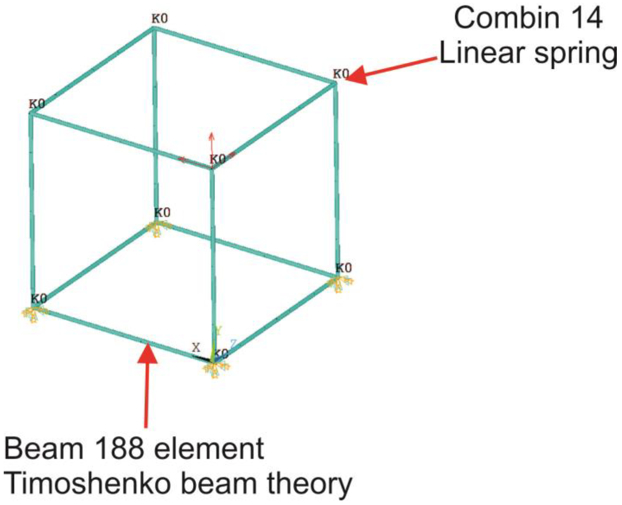
Ansys^® R2022, software was used for the simulations. The models consisted of regular beams with the Thimoshenko formulation (Beam188 element type) and linear elastic elements (Combin14 element type) at the corners (Figure 10).

The stiffness of each elastic element is defined through the real constant value of the corresponding Combin14 elements. Figure 11 presents the distribution of the real constants and the node numbers of the structure. It is noted that each corner is associated with 18 real constant numbers, corresponding to six elastic elements for each converging beam.

2.2. Initial ANN Models

The methodology carried out to train the ANN with the aim of predicting the stiffness values (output) for a set of nodal displacement is presented in the block diagram of Figure 12. First, the stiffness values and the directional displacements and rotations of the corner nodes (1–8) were recorded for each of the 1 × 10⁵ simulations carried out. The process of updating stiffness values, simulating, and storing the data was automatized with a customized APDL script to increase time effectiveness.

The displacement values were subtracted from the reference displacements obtained for a regular beam model in order to isolate the effects of the spring elements.

The resulting displacement values were then fed into different networks, always utilizing 80% of the data to train and 20% of the data to test the network and a total number of epochs of 500.

The rest of the principal characteristics of the network were varied iteratively in order to obtain the most accurate ANN configuration possible (Figure 13):

-

Hidden layers: 1 to 5;

-

Hidden layer nodes: 1 to 1000;

-

Learning rate: 0.01 to 0.001;

-

Activation function: Relu Sigmoid, Linear;

-

Optimizers: gradient descent optimizer (SGD), ADAM optimizer, and RSMProp optimizer.

Python with Tensor Flow and Keras was employed for the simulations of the ANN. As will be explained below, some modifications of the output layer were performed in the network based on the findings of the detailed analysis of converging elastic elements as described in the next section, but the studied ANN parameter ranges were kept unchanged.

From Equation (1), we find that the values of the elastic elements and the displacements are directly related. The elastic elements are integrated in the so-called stiffness matrix of the FEM model:

$$\left\{F\right\}=\left[K\right]\left\{u\right\}\to \left[K\right]=\frac{\left\{F\right\}}{\left\{u\right\}}$$

(2)

Furthermore, if the input forces {F} are kept unmodified among the simulations, the relation between the stiffness values of the elastic elements and the resulting displacements will have an inverse linear relation.

$$\left[K\right]=f\left(\frac{1}{\left\{u\right\}}\right)$$

(3)

On the basis of this straightforward relation between the input and output values, the initial hypothesis was that it should not be a big challenge for an ANN to show satisfactory results, as was especially the case for significant sampling data.

2.3. FEM Theoretical Aspects

The importance of the stiffness matrix in the response of the FEM model was noticeable, and in some way, a properly trained ANN should “learn” how it is constructed in order to predict the resulting displacements. On this basis, a detailed analysis of the stiffness matrix construction is carried out in this section for the specific case where elastic elements are combined with ordinary beam-type elements.

Ultimately, the stiffness matrix represents a fundamental element which determines how every node of every model will behave in every degree of freedom, completely defining the model response. In the most generic case of a two-node elastic element (Figure 14), each with 6 degrees of freedom (DOF), the interaction between each DOF would be given by the stiffness values corresponding to that particular DOF, and Equation (1) would be developed as Equation (4).

$$\begin{gathered} \left\{\begin{array}{c}F1x\\ F1y\\ \begin{array}{c}F1z\\ M1x\\ \begin{array}{c}M1y\\ M1z\\ \begin{array}{c}F2x\\ F2y\\ \begin{array}{c}F2z\\ \begin{array}{c}M2x\\ M2y\end{array}\\ M2z\end{array}\end{array}\end{array}\end{array}\end{array}\right\}=\left[K_s\right]\left\{\begin{array}{c}u1x\\ u1y\\ \begin{array}{c}u1z\\ \theta 1x\\ \begin{array}{c}\theta 1y\\ \theta 1z\\ \begin{array}{c}u2x\\ u2y\\ \begin{array}{c}u2z\\ \begin{array}{c}\theta 2x\\ \theta 2y\end{array}\\ \theta 2z\end{array}\end{array}\end{array}\end{array}\end{array}\right\} \\ {K}_s=\left[\begin{array}{c}kx\\ 0\\ \begin{array}{c}0\\ 0\\ \begin{array}{c}0\\ 0\\ \begin{array}{c}-kx\\ 0\\ \begin{array}{c}0\\ 0\\ \begin{array}{c}0\\ 0\end{array}\end{array}\end{array}\end{array}\end{array}\end{array}\begin{array}{c}0\\ ky\\ \begin{array}{c}0\\ 0\\ \begin{array}{c}0\\ 0\\ \begin{array}{c}0\\ -ky\\ \begin{array}{c}0\\ 0\\ \begin{array}{c}0\\ 0\end{array}\end{array}\end{array}\end{array}\end{array}\end{array}\begin{array}{c}0\\ 0\\ \begin{array}{c}kz\\ 0\\ \begin{array}{c}0\\ 0\\ \begin{array}{c}0\\ 0\\ \begin{array}{c}-kz\\ 0\\ \begin{array}{c}0\\ 0\end{array}\end{array}\end{array}\end{array}\end{array}\end{array}\begin{array}{c}0\\ 0\\ \begin{array}{c}0\\ krx\\ \begin{array}{c}0\\ 0\\ \begin{array}{c}0\\ 0\\ \begin{array}{c}0\\ -krx\\ \begin{array}{c}0\\ 0\end{array}\end{array}\end{array}\end{array}\end{array}\end{array}\begin{array}{c}0\\ -ky\\ \begin{array}{c}0\\ 0\\ \begin{array}{c}kry\\ 0\\ \begin{array}{c}0\\ 0\\ \begin{array}{c}0\\ 0\\ \begin{array}{c}-kry\\ 0\end{array}\end{array}\end{array}\end{array}\end{array}\end{array}\begin{array}{c}0\\ 0\\ \begin{array}{c}-kz\\ 0\\ \begin{array}{c}0\\ krz\\ \begin{array}{c}0\\ 0\\ \begin{array}{c}0\\ 0\\ \begin{array}{c}0\\ -krz\end{array}\end{array}\end{array}\end{array}\end{array}\end{array}\begin{array}{c}-kx\\ 0\\ \begin{array}{c}0\\ 0\\ \begin{array}{c}0\\ 0\\ \begin{array}{c}kx\\ 0\\ \begin{array}{c}0\\ 0\\ \begin{array}{c}0\\ 0\end{array}\end{array}\end{array}\end{array}\end{array}\end{array}\begin{array}{c}0\\ -ky\\ \begin{array}{c}0\\ 0\\ \begin{array}{c}0\\ 0\\ \begin{array}{c}0\\ ky\\ \begin{array}{c}0\\ 0\\ \begin{array}{c}0\\ 0\end{array}\end{array}\end{array}\end{array}\end{array}\end{array}\begin{array}{c}0\\ 0\\ \begin{array}{c}-kz\\ 0\\ \begin{array}{c}0\\ 0\\ \begin{array}{c}0\\ 0\\ \begin{array}{c}kz\\ 0\\ \begin{array}{c}0\\ 0\end{array}\end{array}\end{array}\end{array}\end{array}\end{array}\begin{array}{c}0\\ 0\\ \begin{array}{c}0\\ -krx\\ \begin{array}{c}0\\ 0\\ \begin{array}{c}0\\ 0\\ \begin{array}{c}0\\ krx\\ \begin{array}{c}0\\ 0\end{array}\end{array}\end{array}\end{array}\end{array}\end{array}\begin{array}{c}0\\ 0\\ \begin{array}{c}0\\ 0\\ \begin{array}{c}-kry\\ 0\\ \begin{array}{c}0\\ 0\\ \begin{array}{c}0\\ 0\\ \begin{array}{c}kry\\ 0\end{array}\end{array}\end{array}\end{array}\end{array}\end{array}\begin{array}{c}0\\ 0\\ \begin{array}{c}0\\ 0\\ \begin{array}{c}0\\ -krz\\ \begin{array}{c}0\\ 0\\ \begin{array}{c}0\\ 0\\ \begin{array}{c}0\\ krz\end{array}\end{array}\end{array}\end{array}\end{array}\end{array}\right] \end{gathered}$$

(4)

From this equation, it can be seen that a nodal displacement in the “X” direction will be conditioned by the force applied in that direction and the “kx” stiffness value, evidencing the importance of the stiffness matrix in the characterization of FEM models.

In a similar way, for a generic two-node beam element with 6 DOF per node, as shown in 0, Equation (1) would be developed as Equation (5) Figure 15.

$$\left\{\begin{array}{c}F1x\\ F1y\\ \begin{array}{c}F1z\\ M1x\\ \begin{array}{c}M1y\\ M1z\\ \begin{array}{c}F2x\\ F2y\\ \begin{array}{c}F2z\\ \begin{array}{c}M2x\\ M2y\end{array}\\ M2z\end{array}\end{array}\end{array}\end{array}\end{array}\right\}=\left[K\right]\left\{\begin{array}{c}u1x\\ u1y\\ \begin{array}{c}u1z\\ \theta 1x\\ \begin{array}{c}\theta 1y\\ \theta 1z\\ \begin{array}{c}u2x\\ u2y\\ \begin{array}{c}u2z\\ \begin{array}{c}\theta 2x\\ \theta 2y\end{array}\\ \theta 2z\end{array}\end{array}\end{array}\end{array}\end{array}\right\}$$

(5)

where:

where:

-

I_y, and I_z are the moments of inertia of the beam element along each axis;

-

A and L are the cross section and length of the beam element, respectively;

-

E and G are the elastic and shear modulus of the beam material;

-

ϕ_y, and ϕ_z are material and geometric constants noted as: ${\mathsf{\varphi }}_{\left(i\right)}=12E{I}_{\left(i\right)}/AG{L}^2$.

The terms contained in the stiffness matrix of the beam are composed by the geometrical and material properties of the beam, for example, the term EA/L represents the stiffness under axial load (traction–compression) and is given by the section area of the profile (A), the material’s Young’s modulus (E), and the length of the beam (L).

Extending the analysis to an element composed of a beam and spring element, such as the one shown in Figure 16, three nodes, with 6 DOF per node, were obtained and Equation (1) would be developed as Equation (6).

$$\begin{gathered} \left\{F\right\}=\left[K_{sb}\right]\left\{X\right\} \\ \left\{F\right\}={\left\{F_{1x} F_{1y} F_{1z} M_{1x} M_{1y} M_{1z} F_{2x} F_{2y} F_{2z} M_{2x} M_{2y} M_{2z} F_{3x} F_{3y} F_{3z} M_{3x} M_{3y} M_{3z}\right\}}^T \\ \left\{X\right\}={\left\{u_{1x} u_{1y} u_{1z} {\theta }_{1x} {\theta }_{1y} {\theta }_{1z} u_{2x} u_{2y} u_{2z} {\theta }_{2x} {\theta }_{2y} {\theta }_{2z} u_{3x} u_{3y} u_{3z} {\theta }_{3x} {\theta }_{3y} {\theta }_{3z}\right\}}^T \end{gathered}$$

(6)

where:

where k_1x, k_1y, k_1z, k_1rx, k_1ry, and k_1rz are the 6 stiffness values of the elastic element.

In this case, the stiffness matrix has 3 nodes × 6 DOF per node = 18 × 18 elements. The green region corresponds to node 1 and depends on a spring behavior, the orange region corresponds to node 3 and depends on a beam behavior, and finally, the blue region corresponds to the midnode that depends on both the beam and spring having its stiffness values added. For example, for node 2, an axial load will have a stiffness value of k_1x + AE/L.

The proposed alternative beam element would have a total of 4 nodes with 6 DOF, leading to a stiffness matrix of 24 × 24 with two midnodes with mixed influences of beam and spring elements. For the sake of simplicity, the complete stiffness matrix of this element is not included in the document.

In the FEM simulations of the cube structure, the material and geometry characteristics were kept unmodified. Therefore, the terms in the stiffness matrix corresponding to the beam element did not change, and the only modifications that took place were as a consequence of the 144 stiffness values that were randomly modified, as explained before.

Based on this development, the corner floating nodes of the cube structure would be equivalent to node 1 in Equation (5) for each of the three concurrent elements. Therefore, the stiffness of the elastic elements of each element would be added, leading to an equivalent value that will characterize the displacement of the floating node.

2.4. Final ANN Configuration Based on the Stiffness Behavior Evaluation

Based on the analysis presented above, it is possible to reduce the number of input parameters that feed the ANN by using the equivalent stiffness values determined in Equation (7). In this equation, subindex “i” refers to the ith floating node (1 to 8), and subindexes 1 to 3 are given indistinctly to each of the three nodes concurring in the corner.

Given that if these equivalent stiffnesses are equal, the resulting displacements obtained on the FEM model will also be equal, by implementing the equivalent stiffness values, we avoid feeding the ANN with different input combinations that lead to the same results.

$$\begin{gathered} \forall \left[\begin{array}{c}{k}_{ux},k_{uy},k_{uz}\\ k_{rotx},k_{roty},k_{rotz}\end{array}\right]\in N\left(1\cdots 8\right) \\ \begin{array}{c}{ke}_{ux}=k_{ux1}^{N\left(i\right)}+k_{ux2}^{N\left(i\right)}+k_{ux3}^{N\left(i\right)}\\ {ke}_{uy}=k_{uy1}^{N\left(i\right)}+k_{uy2}^{N\left(i\right)}+k_{uy3}^{N\left(i\right)}\\ \begin{array}{c}{ke}_{uz}=k_{uz1}^{N\left(i\right)}+k_{uz2}^{N\left(i\right)}+k_{uz3}^{N\left(i\right)}\\ {ke}_{rotx}=k_{rotx1}^{N\left(i\right)}+k_{rotx2}^{N\left(i\right)}+k_{rotx3}^{N\left(i\right)}\\ \begin{array}{c}{ke}_{roty}=k_{roty1}^{N\left(i\right)}+k_{roty2}^{N\left(i\right)}+k_{roty3}^{N\left(i\right)}\\ {ke}_{rotz}=k_{rotz1}^{N\left(i\right)}+k_{rotz2}^{N\left(i\right)}+k_{rotz3}^{N\left(i\right)}\end{array}\end{array}\end{array} \end{gathered}$$

(7)

The resulting ANN schema would be as shown in Figure 17; the initial 144 output values are composed of 14 equivalent output values. The rest of the configurations of the ANN were explored as described in Section 2.2.

Tensor Flow Keras ANN

Once we completed the 1 × 10⁵ simulations, numerous ANN configurations of ANN were tested within the parameters’ ranges listed in Section 2.2. Although most of them showed very similar results, the three that led to the most relevant results are summarized in

Table 1. ANN Tensor Flow configurations.

Config.	ANN Model	Nr. Layers	Nodes	Optimizer	Learning Rate	Losses	Metrics	Activation Function	Discussion
1	Sequential	3	48-48-48	SGD	0.01	Mean squared error	Mean absolute error	Linear	Standard configuration for exact mathematical problems; the activation function was selected as linear since the analyzed problem is linear
2	Sequential	3	48-1000-48	SGD	0.01	Mean squared error	Mean absolute error	Linear	Increase the number of nodes in order to increase the prediction capability
3	Sequential	3	48-48-48	SGD	0.0001	Mean squared error	Mean absolute error	Linear	By decreasing the learning rate, the learning curve should be more robust and consistent

and will be presented in more detail in the Section 3.

Due to the large number of data analyzed, the computational requirements were significant for some ANN configurations. This issue was solved by utilizing Google Colab, which provides high computational resources at reduced costs, determining the necessity of programming the ANN with Tensor Flow.

3. Results and Analysis

In this section, further results and analysis are presented for the three combinations gathered in Table 1. The significant amount of information on the results that was obtained should be taken into consideration, corresponding to the 48 output values coming from the “k” predictions. Thus, for the sake of clarity, redundant information from different stiffness estimations will not be included in the document.

3.1. Results Obtained for the ANN Configuration 1

The evolution of the mean squared error for both the training and validation data is shown in Figure 18. The decreasing tendency of both errors as the epochs advance suggest that the ANN seems to be able to learn.

On the contrary, analyzing the predictions of the ANN for the stiffness values, unsatisfactory results were obtained both for training and testing data. A sample of these results is shown in Figure 17 for training (left-side graphs) and testing (right-side graphs) data for K_xrot(5), K_y(7), and K_zrot(8), in which the reference correct values are marked in blue and the ANN estimated values are marked in red. As can be seen, neither the training nor predictions provided good results; for some of the output variables, we have a higher dispersion, but in all of the cases, the averages are centered on the median value.

3.2. Results Obtained for the ANN Configuration 2

Figure 18 presents the evolution of the absolute mean squared error for training and validation data. A similar decreasing tendency with respect to configuration 1 can be observed, although with better initial estimation results for the initial epochs in this case.

Again, the results obtained for this third configuration were not satisfactory; the ANN was learning up to 500 epochs and even showed a tendency to keep learning. Nevertheless, when the results for the predictions of stiffness values were analyzed, it was clearly observed that the ANN was not capable of providing good estimations and that the predicted values were once again centered around the average value, although with a lower dispersion with respect to configuration 1. These results are shown in Figure 19 for the same stiffness values for comparison purposes Figure 20.

3.3. Results Obtained for the ANN Configuration 3

Figure 18 presents the evolution of the absolute mean squared error for both the training and validation data for the fifth ANN configuration. With respect to the previous configurations, the decreasing rate of the error was higher and seemed to stabilize from 200 to 250 epochs. Also, the error values reached were significantly lower compared to the previous configurations.

Conversely, observing the results of the stiffness estimation (Figure 21), no significant improvement can be observed with respect to the previous configurations. Bigger dispersion was noted, suggesting that the estimations attempted to perform differentiated behavior, but were still centered around the average value with notable deviations from the reference correct values Figure 22 and Figure 23.

3.4. Additional Analysis and Results

Given the unpredictable results obtained and that no significant improvements could be obtained for the different ANNs tested, a deeper behavioral analysis was carried out to investigate the correlations between the inputs (displacements) and outputs (equivalent stiffness values). To perform this, the 48 obtained nodal displacements were plotted against each one of the 48 equivalent elastic element values resulting in 48 × 48 = 2304 graphs to analyze the correlations. For clarity’s sake, only representative examples of the findings of the present analysis will be included in the paper.

As was expected for embedded nodes 1–4, the modification of the elastic elements did not have any influence on the displacement values, regardless of the elastic values. By way of example, this behavior is shown in Figure 24 for the Uz displacement of node 1 with respect to the RotZ equivalent stiffness value of node 5. A zero-centered vertical line can be noted, meaning that the Uz displacement will be null regardless of the stiffness value selected.

Surprisingly, when analyzing the correlations for the nonembedded nodes (5 to 8), it was observed that the input and output values were hardly correlated; in fact, for the vast majority of the cases, no correlation could be identified at all.

To illustrate this, the first left-handed graph of Figure 25 shows the Ux displacement of node 5 in relation to the RotZ equivalent stiffness of node 2, where no correlation can be identified at all. Similarly, the center graph plots the RotZ rotation of node 8 in relation to the RotZ equivalent stiffness of the same node, where no correlation can be observed either. These are two examples of the most common behavior observed for the different input–output plots analyzed.

Conversely, a few parameters showed recognizable correlation, especially for low values of stiffness. For example, the right graph of Figure 25 relates the Uz displacements of node 5 with respect to the Uz equivalent stiffness values of the same node, where a clear correlation was detected for smaller stiffness values. This correlation decreases significantly and becomes almost unnoticeable for high stiffness values.

The analysis was extended to increased stiffness values, or even analyzing additional nodes not located in the corners, but the obtained results were the same.

Due to the deterministic nature of FEM, it seems clear that the modification of one stiffness value will lead to a modification of the displacements, following Equation (1). Nevertheless, it seems that the effect of the different stiffness values might compensate each other, resulting in unobservable input–output correlations.

In this scenario of a general lack of correlation, the relation between the displacements and the stiffness values very closely resembles a random or pseudorandom distribution, which indeed seems a drawback for an ANN in learning how to estimate outputs based on inputs. To prove this hypothesis, a specific ANN was constructed and trained based on completely random input and output values. The results obtained are shown in Figure 26, where a very significant similarity with those obtained in the displacement–stiffness ANNs can be noted. It seems that for random data, without input–output correlation, the best solutions for an ANN that minimizes the errors is to center the estimations to the average values of the correct output.

These observations present a challenge in order to understand how the data generated from a precise FEM model could have no correlation, especially taking into consideration the fact that the relation between the elastic elements and nodal displacements is linear and programmed into the FEM software Ansys® R2022.

Further analysis of the FEM model confirmed that any modification of any of the stiffness values resulted in a modification of all of the nodes’ displacements. This influence is obviously more pronounced in the proximity of the modifications and for specific directions, but takes place in all the nodes. In this regard, Figure 27 presents a comparative overlaying FEM result generated by the superposition of the deformed shape of the structure without the modification and after the modification of the node 3 RotX elastic element. A modification of the response of the structure can be noted, especially on the zoomed corner, although it affects all nodes’ displacements.

This characteristic stands at the base of the FEM theory and represents a fundamental aspect of this mathematical methodology.

Finally, the analyzed cube had a total of 140 nodes, leading to a total of 140 × 6 = 840 DOF; in this way, in order to obtain a complete characterization of the structure, the FEM model was required to calculate 840 displacement values in comparison to the proposed ANN, in which just 48 displacement values were utilized.

4. Conclusions

This paper presents a novel, generally improved beam model, marking a significant advancement in the field of structural modeling. This model is characterized by 4 nodes, 12 elastic elements, and 1 beam, in stark contrast to the conventional beam elements that comprise only 2 nodes and 1 element. This innovation enhances the adaptability of modeled structures at the joint level and necessitates a novel methodology for the precise estimation of elastic elements at the joint level.

The model is based on the addition of elastic elements to a joint of concurrent beams, making it capable of characterizing its stiffness behavior irrespective of the joint type. The main challenge in developing this model was determining the stiffness values of the newly introduced elastic elements, for which we explored the capability of artificial neural networks (ANNs) in this paper.

The case study is a simple cube-shaped structure with a total of eight corner junctions in which elastic elements stiffness are randomly modified and the resulting displacement is recorded to be used as input data for training the ANN.

A wide variety of ANN configurations were explored, obtained by modifying the number of hidden layers and neurons, the learning rate, the activation function, and the optimizer. The following conclusions were obtained:

-

In general terms, unexpectedly, the different ANNs evaluated led to similar unsatisfactory results, with a clear tendency to center the predictions on the average of the correct values, with slight variations in the dispersion depending on the ANN configuration.

-

Further analysis performed revealed that this behavior is noted in the ANN when the input and output data samples are random (i.e., with no correlation between them). This lack of correspondence was clearly observed between most of the displacements (input) and stiffness values of the elastic elements (output) on the calculated structure. Apparently, in such a situation the best prediction that the ANNs achieve to minimize the errors is to center on the average of the correct outputs.

-

The limitations of using ANNs for general predictions of FEM models’ responses were evidenced based on a few nodal data, where crossed effects might not be characterizable and only pseudorandom responses can be obtained.

-

Alternatives focused on an increased representation of the stiffness matrix in the ANN training data (i.e., more nodal displacement results) might be explored, although the authors cannot provide a guarantee of success, and would certainly suppose a significant increase in the ANN complexity and consequent computational costs.

In any case, the findings provided in the present work represent a contribution in itself to the state of the art of the scientific knowledge regarding the connection between artificial neural networks and the finite element method, and the information is valuable to be employed in continuing engineering and research projects on this field.