Abstract
In this communication, the solution of the differential Riccati equation is shown to provide a closed analytical expression for the transient settling velocity of arbitrary non-spherical particles in a still, unbounded viscous fluid. Such a solution is verified against the numerical results of the integrated differential equation, establishing its accuracy, and validated against previous experimental, theoretical and numerical studies, illustrating the effect of particle sphericity. The developed closed analytical formulae are simple and applicable to general initial velocity conditions in the Stokes, transitional and Newtonian regimes, extending the range of application of former published analytical approximate solutions on this subject.
Keywords:
Riccati differential equation; closed analytical solution; non-spherical particle; unbounded viscous fluid; settling velocity MSC:
34A05
1. Introduction
The Riccati equation is one of the simplest non-linear first-order ordinary differential equations (ODEs). It possesses the general form:
where is the independent variable, is the unknown function depending on and are the known coefficients which, in general, vary with .
Apart from its intrinsic interest as a non-linear equation, the Riccati equation arises in many applications in physics, engineering and mathematics. For instance, it appears in control theory [1], Newtonian dynamics [2], quantum mechanics [3,4], reactor Engineering [5], cosmology [6] or financial mathematics [7], among others.
Riccati equation and its solution methods are usually included in the handbooks dealing with ODEs (e.g., [8,9,10,11]). Despite many solutions of such an equation are known, there is no general procedure to find its analytical solutions [12]. However, there are specific situations where it is possible, for instance, if a particular solution is known. In this case, it is possible to derive a new solution that satisfies a Bernoulli equation, which can be solved analytically [13]. If the independent variable represents time and the particular solution satisfies that its time derivative is zero, such a particular solution is just the steady-state solution of the system. An example of that situation was given in [5], in the context of ideal environmental reactors.
In the present contribution, it is shown that, under certain restrictions, the sedimentation velocity of a heavy particle falling in a quiescent fluid also satisfies a Riccati equation, whose analytical solution is developed in the following. In this context, a reliable estimation of the accelerated movement of objects, whether spherical or non-spherical, immersed in fluids is needed in a number of engineering applications. Examples are flotation, separation of liquid–solid suspensions, fixed or fluidized bed reactors and gravity-induced collection or classification. In particular, particle separation plays a crucial role in various applications, including municipal solid waste treatment (e.g., clarifiers), mineral preparation, agricultural raw material cleaning (such as coffee beans, fibers, grains and nuts) and final product design, among others. To accomplish this task, a wide range of devices and industrial apparatuses are employed, such as screw, zigzag and counter-current classifiers, as well as cyclones. In order to develop the design and improve the operation or troubleshooting of such processes and equipment, it often becomes necessary to have detailed knowledge not only about the particle terminal velocities but also of the trajectories followed by the accelerating bodies. In some other applications, ascertaining the time and distance that a particle needs to reach its terminal velocity is crucial, such as in the case of drinking water clarifiers, liquid viscosity measurement by the sediment sphere technique or the estimation of raindrops’ terminal velocity. This knowledge is vital for making accurate determinations of the settling velocity of the object.
To describe the unsteady behavior of a sedimenting body in a still fluid, apart from numerical solutions, analytical methods have also been employed, e.g., [14,15,16,17,18,19]. For instance, Ref. [20] developed an analytical solution for the sedimentation velocity of a spherical particle in a fluid medium at rest. The main hypotheses were that the drag coefficient could be given according to the Rubey law, and the Basset history term can be assimilated as an inertial force and be combined with the added mass in an integrated term. The first hypothesis is evaluated and partially corroborated against experimental data of [21] and the second one is assumed based on the numerical simulations of [22], which suggested that the added mass and Basset forces show a similar trend and temporal variation. The obtained solution was compared favorably versus the experimental data of [23,24]. The authors of [25] developed analytical solutions for the settling velocity of spherical particles in the Stokes and Newton regimes as limiting cases but without considering the history force or the transitional regime. Later, in [26], experiments were conducted considering the transitional regime and then compared with numerical solutions and the closed expressions provided by [25]. They found deviations between their experiments and the analytical formulae in the Reynolds Range , but a good match with the numerical results. Very recently, in Ref. [27], the authors discussed the effects of Basset force on the settling of spherical particles from an experimental point of view and concluded that the heuristic approach of [20] is appropriate. Additionally, these authors provided a correlation of the history force coefficient with the Archimedes number. Also, the recent contribution of Kalman and Matana [28] provided a comprehensive review of terminal velocities for spherical particles.
Regarding non-spherical particles, the studies dealing with analytical approaches to solve the BBO (Basset–Boussinesq–Ossen) equation usually employ the Chien drag law [29], which depends on particle sphericity [30,31,32,33]. Sphericity is defined as the quotient of the superficial area of the spherical particle which has the same volume as the real particle and the surface area of that particle [34]. In this context, different analytical techniques that approximate the solution as an infinite power series have been developed. For instance, the Variational Iteration Method (VIM) was applied by [30] to obtain an approximated analytical solution of the unsteady motion of a non-spherical particle in an incompressible Newtonian fluid for a wide range of Reynolds numbers. Another approximate technique, the Differential Transformation Method (DTM), was employed in [31] to find analytical expressions for the unsteady velocity and acceleration of non-spherical particles immersed in various Newtonian liquids. Their results were compared and validated with those of VIM and numerical solutions obtained using the fourth-order Runge–Kutta method. The Homotopy Perturbation Method (HPM) is another analytical method that has been applied to obtain expressions describing the accelerating motion of sedimenting particles in liquids. A variant of it, called the Optimal Homotopy Analysis Method, is introduced in [32] and implemented to describe the transient motion of a rigid particle sinking in a still viscous fluid. The resulting analytical expression, built using a different number of terms in the series, compared favorably with numerical solutions based on Runge–Kutta methods. In [33], HPM combined with Padé approximants was applied to investigate the falling motion of nano-droplets in quiescent viscous media with an initial velocity and compared their results with those obtained by VIM and numerical solutions, showing good agreement. All the mentioned methods provide analytical approximations to the solutions, which are either fairly complex or excessively extensive and not well suited to be implemented for design and control processes [25]. Actually, such approximation of solution by power series needs many terms to get accurate estimations of particle settling velocities whose number cannot be known beforehand; for instance, Ref. [31] employs 10 or more terms, Ref. [30] uses 14 terms and [32] uses between 15 and 30 terms. Therefore, to overcome such limitations, this contribution develops a closed analytical expression for the unsteady sedimentation velocity of non-spherical particles, along with their corresponding acceleration and displacement, in a quiescent Newtonian fluid; the obtained solution is simple, applicable to general initial velocity conditions and in the Stokes, transitional and Newtonian regimes.
The structure of this communication is the following. Section 2 presents the formulation of the problem together with the main simplifying hypothesis and develops the closed analytical solutions for particle velocity, acceleration and displacement. Paragraph 3 exposes some reflections on the relevance of the history force on particle acceleration and how its effects can be incorporated into the description of particle motion. Provided analytical solutions for particle velocity, acceleration and falling distance are verified against numerical solutions of the Riccati ODE and validated versus previous experimental, theoretical and numerical results available in the literature in Section 4. Finally, the conclusions of the study are exposed in the last part, summarizing the main advantages and limitations of the present study.
2. Problem Statement and Development of the Closed Analytical Solution
This section first presents the particle general motion equation introducing all the relevant physical variables. Under certain assumptions, adequately identified, it is transformed into a Riccati ODE for the settling velocity, given by Equation (1). Next, the process for obtaining the closed analytical solution is properly described, which eventually allows obtaining a compact expression for the unsteady particle velocity, Equation (13). From that solution, the body acceleration and displacement are obtained by derivation and integration, respectively. Finally, a short discussion of the settling motion’s relevant time and spatial scales is performed.
The motion of a non-spherical rigid particle, of sphericity , sedimenting in an unbounded still fluid can be described by the Basset–Boussinesq–Ossen (BBO) equation, which reads [35]:
In Equation (2), is the particle mass, is the fall velocity depending on time , the sphere equivalent diameter (i.e., the diameter of a sphere with the same volume that the actual particle), the gravity acceleration, and the fluid and particle densities, respectively, and the fluid dynamic viscosity. Also, is the drag coefficient and is the virtual mass coefficient. The terms on the right-hand side represent, from left to right, the forces of weight-buoyancy, drag, virtual mass and Basset or history force.
In the expression of the drag force in Equation (2), the factor represents the projected area of the non-spherical particle based on the particle equivalent diameter , which is the customary choice. However, this factor can be substituted by if the actual value of the projected area is known. For instance, regular non-spherical particles, such as ellipsoids or cylinders, tend to settle down, keeping their maximum projected area orthogonal to the direction of the motion [36,37], thereby maximizing the experienced drag. In such cases, it is possible to repeat the process described in the next paragraphs to obtain particular expressions of the settling velocity of definite non-spherical shapes.
Furthermore, the history force deserves a comment. It represents a memory term representing the “additional viscous force on the particle during the unsteady motion, which describes the diffusion of vorticity around the particle during its whole history” [38]. In this form, the particle motion equation, Equation (2), is an integro-differential equation that must be solved by numerical methods. In certain situations, such as a heavy particle falling in a gas, where , the Basset term can be neglected [39].
In such a case, without the history force, Equation (2) can be cast into the form:
Different drag laws for spherical particles in transitional flow have been developed empirically [22,40,41,42], but the one that stands out, due to its simplicity and accuracy, is the so-called Rubey’s drag law [43]. The latter is a two-parameter empirical correlation that can be expressed as:
where is the particle Reynolds number. The values of and are adopted to maintain consistency with the drag laws in the Stokes and Newton regimes in the case of spherical particles as follows: [20]. Rubey’s expression also compares favorably with data of non-spherical particles of natural sediments for certain choices of and [20,30]. In this latter case, it is customary to describe the non-sphericity of particles by the sphericity parameter , introduced previously. In this context, one well-known analytical correlation between Reynolds numbers and drag coefficient for non-spherical bodies is presented by Chien [29]
which is said to be valid in the sphericity range of and for Re < 5000. The functional form of Equation (5) is the same as Equation (4), where the parameter is a function of particle sphericity. It has the advantage of not including additional non-linearities in the drag coefficient, and it has been used in previous works dealing with non-spherical particles [30,31,32,33]; therefore, Equation (5) will be applied in this work to obtain closed analytical solutions of the particle motion equation, Equation (3).
Now, plugging the expression of Equation (4) in Equation (3), it is obtained:
where is the kinematic viscosity of the fluid. Defining and dividing all terms by the coefficient of the time derivative on the left-hand side, Equation (6) is finally expressed in the form:
Equation (7) corresponds to the general Riccati equation, Equation (1), with with constant coefficients:
Let us observe that all physical variables are positive, so and are negative, and with the previous definition and are positive values. Moreover, according to their definition, coefficients and H do not depend on time; therefore, they take constant values for a specific fluid-particle system.
In the present case, we easily obtain a particular solution of Equation (7), , corresponding to the steady-state terminal velocity of the particle. It is written in terms of the positive parameters and :
In the case of a heavy particle, , and the plus sign in front of the square root provides the physical solution of positive terminal velocity. Let us notice that the value of the terminal velocity is constant for each particular particle–fluid system and is not affected by the transient forces as it arises from the equilibrium between the steady drag and gravity–buoyancy forces.
Starting from the particular solution, Equation (9), the general solution of the Riccati Equation (7) can be obtained as indicated in [5]. The final result is the following:
In Equation (10), is the particle initial velocity with which it is released within the fluid, which can be zero or non-zero. It is readily seen that for , the second addend on the right-hand side (RHS) vanishes and only the steady-state solution remains, i.e., the particle moves with its terminal velocity. Additionally, for , it is easily seen that .
Let us introduce the following notation:
where the second equality follows from expression, Equation (9). Then, solution (10) is immediately written as:
Performing the corresponding operations inside the square bracket, a compact formula for the particle velocity is finally obtained:
where coefficient includes the information about initial conditions. Equation (13) shows that the fall velocity of a particle can be obtained by subtracting a transient function from its terminal velocity. Such a function starts from the value at and evolves exponentially to zero. In other words, the particle velocity increases or decreases if the initial velocity is larger than , exponentially up to reaching its terminal velocity.
It must be emphasized that obtained solution for is determined by the drag law expression, Equation (5), whose coefficients, , do not depend on the particle Reynolds number. If other drag expressions involving such dependence are to be used, e.g., [40,42], a closed analytical solution will likely not be possible and Equation (3) must be solved numerically.
The acceleration of the particle is readily computed from the solution (13) just deriving it with respect to time:
The falling distance is obtained by integrating (13) by introducing the substitution . Therefore, and the function in Equation (13) can be integrated as:
where the second equality follows after decomposing by partial fractions. The result is transformed back to the primitive variable and applying the properties of logarithms:
Then, the falling displacement is
and using Equation (11), the final result is cast into the final form:
This section is finished by highlighting some characteristic scales of the settling motion. Looking at Equation (8), it is seen that represents the inverse of a length scale, the inverse of a time scale and is interpreted as an acceleration scale imposed by the external gravity field. Looking at the definition of , it is the exact expression for the inverse of the Stokesian particle relaxation time [26]; therefore, represents a Stokesian frequency. On the other hand, in the Newtonian regime of motion (i.e., ), the terminal velocity is given by:
Following [26], the characteristic Newtonian time scale is written as:
whose inverse is a Newtonian frequency. Therefore, a Newtonian length scale is built as:
Consequently, constitutes a Newtonian inverse length scale. The coefficient of in the argument of the exponential, , can analogously be interpreted as an inverse time scale or frequency of the particle settling motion. By its definition, it is built from the Stokesian and Newtonian frequencies as , i.e., it is a kind of weighted quadratic mean of both frequencies.
Then, the characteristic velocity scale of the settling motion appearing in Equation (13), , is a mixed scale: the Newtonian length scale over the settling motion time scale . It is easy to see from Equation (13) that such a velocity scale is larger than the terminal velocity . In this context, the characteristic acceleration scale of the settling motion is the settling velocity scale over the time scale, i.e., .
In the case of settling distance Equation (15), substituting in terms of frequencies and from Equation (9) and operating, it is found that:
where it is seen that the settling distance is computed as the Newtonian length scale multiplied by a function depending on . In such a function, two frequencies appear: the settling frequency and the average of the Stokesian and settling frequencies.
3. A Comment on the Role of the Basset History Force
The role of the Basset force in particle motion equation has been widely discussed in the open literature. As it has been seen, its consideration renders the particle motion equation an integro-differential equation, not amenable to an analytic solution. In practice, there are some physically meaningful situations, where such force can be safely neglected, such as gas–solid particle flows [39,44]; but in general, it plays a non-negligible role in the particle unsteady motion in laminar and turbulent flows [45]. Nevertheless, in the context of the application considered in the present study, several authors have argued that apart from its viscous origin, due to the explicit appearance of the viscosity in its formulation, the Basset term also could be associated with inertial effects (e.g., [22]). In fact, Ref. [20] heuristically combined the added mass and history forces in an integrated term after arguing that in the computations of [22] both forces show similar trends in their time evolution. Thus, Ref. [20] assimilated the effect of the history term to that of virtual mass by effectively increasing the added mass coefficient; this assumption was supported by the fact that its theoretical prediction for spherical particles compared more favorably with the experimental data of [23,24] when was increased from 0.5 to 2.0.
A very recent article, Ref. [27], after a systematic experimental study, found that Basset force is significant at the start of spherical particle settling but decays to zero during motion. This fact contradicts the results obtained by numerical computations of such force as it starts as zero in the beginning of movement, increases rapidly and finally decreases softly to vanishingly small values. Based on their experimental results, Ref. [27] favors the idea of the heuristic formulation of a history force proportional to particle acceleration through a coefficient that is well correlated with the Archimedes number, , of the system. Finally, the authors of [27] provide the parameter region, where history force is important as that with .
The previous discussion supports the empirical inclusion of history force effects in the particle motion equation as an inertial effect amenable to be combined with the virtual mass term, keeping it simple enough to be tractable by analytical approaches. Actually, various works have employed such an approach, for instance [31] or [35]. The straightforward consequence is that the solution presented in Equation (13), strictly obtained without including the Basset force, can heuristically incorporate such an effect by simply modifying the value of the coefficient. Therefore, when comparing with previous studies, the value of this coefficient must be specified.
4. Comparison of Results with Previous Studies and Experiments
In this section, the obtained expressions of particle velocity, Equation (13), acceleration, Equation (14) and falling distance, Equation (15), are compared and validated against experimental and numerical previous results. Moreover, in the present contribution, a numerical solution of Equation (7) has been carried out using the fifth-order Runge–Kutta ODE solver of Matlab, ode45. The obtained numerical results are compared, as additional verification, with the evaluation of the analytical solution given by Equation (13), allowing the estimation of its accuracy.
The first case considered for verification and validation is the classical experimental case of Allen [23]. In such experiments, the settling velocity and distance were measured for a spherical steel sphere sedimenting in a prismatic water tank. The relevant physical properties are as follows [20]: m2/s, mm, , , , . Particles start their motion with zero initial velocity, m/s. Further details on the experiment can be found in the original publication.
Figure 1 shows the obtained results in this case. Figure 1a presents the verification study, where the analytical expression, Equation (13), is evaluated for a time interval between 0 and 0.4 s. The resulting function is compared with the numerical results computed using the mentioned Runge–Kutta method (RKM). To quantitatively compare the agreement of both curves, the time-dependent relative error measure is introduced:
where and stand for the analytical and numerical velocity values, respectively. From that, the maximum and mean relative errors are defined as the maximum and averaged values of in the time interval.
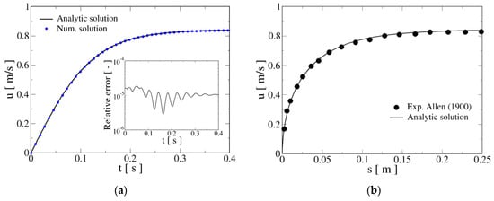
Figure 1.
Verification and validation of the time evolution of falling velocity for the experiments in [23]. (a) Analytical versus numerical settling velocities; the inset shows the evolution of the relative error . (b) Comparison of analytical and measured sedimentation velocities versus displacement curves.
As it can be readily appreciated from Figure 1a, the line representing the analytical curve lies over the full symbols depicting the numerical values calculated by RKM. Inset in Figure 1a displays the temporal evolution of the relative error, which shows an oscillatory behavior. The maximum and mean error measures, in this case, are and indicating an excellent agreement between both solutions.
Figure 1b shows the validation of presented closed analytical formulae with the experiments in [23]. In such a figure, the curve settling velocity versus displacement is compared with the experimental measurements. The analytical curve was constructed by taking the displacement given by Equation (15), evaluated at the corresponding time values, as a horizontal coordinate, and the velocity provided by Equation (13), computed at the same temporal points, as a vertical coordinate. As it can be readily seen, the agreement is satisfactory.
Next, the experiments of Yin et al. [35] are considered. These authors performed measurements of falling spherical plastic and glass particles in tap water at the Hydraulic Laboratory at Ocean University of China. A video camera was employed to record the particles’ falling process after they were released from the surface of the water, and video player software was used to determine the time and distance of each frame.
For illustration purposes, three cases of [35] labeled as Scenarios 1, 2 and 3 have been chosen for comparison; they are given in Table 1. Water density and kinematic viscosity are taken as kg/m3 and m2/s; given in Table 1 stands for the Reynolds number based on particle terminal velocity.

Table 1.
Parameters for the experimental cases of Yin et al. [35].
Values of the coefficients in Rubey drag law were adopted as and , following the settings of [35].
Figure 2 shows the obtained results for the settling velocities (Figure 2a) and displacements (Figure 2b) for the three scenarios. Experiments of [35] only provide measurements of the falling distance versus time and not velocities; however, a verification study is performed comparing the analytical and numerical curves provided by Equation (13) and computed by RKM, respectively. As it can be readily seen from Figure 2a, both graphs superimpose; the corresponding relative error measures are presented in Table 2. It is seen that the error grows moderately as terminal velocity increases, but keeping values of the order of , i.e., of 0.001%. Therefore, it can be concluded that the agreement between numerical and analytical velocities is excellent.
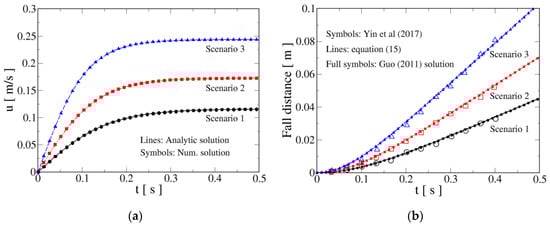
Figure 2.
Verification and validation of the time evolution of falling velocity and displacement for the experiments in [35]. (a) Analytical (lines) versus numerical (symbols) settling velocities. (b) Comparison of falling distance versus time evaluated by Equation (15), with the experimental results of [35] and the solution provided by [20].
Table 2.
Error measures for the considered experimental scenarios of [35].
Figure 2b displays the comparison between the results of settling distance versus time obtained with Equation (15) (lines), experiments (hollow symbols) and those obtained with Equation (32) of Guo [20] (small full symbols). As it can be appreciated, the experimental points are satisfactorily fitted by the results of the function in Equation (15). Moreover, as shown by [35], the experimental curves are well described by the Guo expression. In fact, lines and small full symbols overlap, as should be expected from the closed analytical solution developed in this study.
The theoretical and numerical results of [31] on the falling behavior of non-spherical particles in a still fluid constitute a third validation test for expressions Equations (13) and (14). The authors of [31] solve the simplified BBO equation, Equation (3), where the effect of the Basset force is incorporated in the value of the coefficient, in connection with Chien drag law, Equation (5), appropriate for non-spherical particles. Such drag expression considers the dependence on particle sphericity in the Newtonian regime, i.e., . The employed analytical approach in [31] is the differential transformation method which allows construction of the particle settling velocity as an infinite power series in time. Actually, such authors derive explicitly the first eight terms, which they compare with high-order Runge–Kutta numerical solutions of particle motion equation.
Yaghoobi and Torabi [31] provide the curves versus time for settling velocity and acceleration of non-spherical particles with sphericities in several liquids such as water, ethylene-glycol and glycerin. Here, for brevity, the results of the validation are presented only with water as a fluid, but the same level of agreement is reached with the other liquids. The values of the fluid properties are density kg/m3 and dynamic viscosity kg/(m s). The particle equivalent diameter is mm and its density kg/m3. Finally, the adopted value of the virtual mass coefficient is [31]. Particles are released with zero initial velocity.
In this case, Equation (7) is solved also by the RKM, providing a very good matching with the analytical evaluation of Equation (13) for the settling velocity. Such graphical comparison is not shown here for the sake of brevity, but the error measures are provided in Table 3, whose values are somewhat higher but still comparable to those obtained previously in the cases of [23,35], indicating again a satisfactory agreement between numerical and analytical approximations.
Table 3.
Error measures for the experiments of [31].
Figure 3a shows the comparison between the results of [31] and those obtained from Equation (13) for the four considered values of sphericity. The agreement is excellent. It is seen that the terminal velocity decreases with decreasing sphericity, which is related to the fact that the drag force experienced by a non-spherical particle increases with reducing ; in the present framework, this is reflected in that the Newton drag coefficient in Equation (5) is a decreasing function of sphericity. Moreover, from Figure 3a, it is noticed that the time needed to reach the terminal velocity augments as grows.
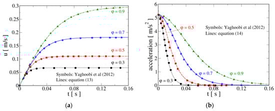
Figure 3.
Comparison of the time evolution of falling velocity, Equation (13), (a) and acceleration, Equation (14), (b) with the results of [31]. The effect of particle sphericity on both variables can be clearly observed in the figures.
Figure 3b presents the behavior of particle acceleration as a function of sphericity comparing the results of [31] and those given by Equation (14). Again, the corresponding curves overlap; from that figure, it is seen that, although the initial acceleration is the same, decreases faster for low sphericity particles. Consequently, the time during which particles experience a non-zero acceleration increases with growing .
To conclude, it has been illustrated that the obtained closed analytical expressions for settling velocity, acceleration and falling distance agree with previous numerical and experimental data for both, spherical and non-spherical particles. These results validate the solutions of the Riccati differential equation developed in this contribution for non-spherical particles sedimentation in a stagnant viscous fluid.
5. Conclusions
The present study has provided a closed analytical solution for the problem of the sedimentation of a general non-spherical particle in a still viscous fluid. It has been demonstrated that, under certain common assumptions, the particle motion equation (BBO) becomes a Riccati non-linear ordinary differential equation. Such equation possesses a steady-state solution, i.e., the terminal velocity of the particle in the fluid, from which the general solution for the particle velocity is constructed, Equation (13), which is valid in the Stokes, transitional and Newton regimes, for zero and non-zero initial conditions, increasing or decreasing velocities. Such a solution relies on the use of Rubey’s drag law, Equation (4), in combination with Chien expression, Equation (5). From the expression for , the corresponding acceleration and fall distance are obtained by direct derivation and integration, respectively. In particular, in the case of non-spherical particles, the provided closed analytical functions are simple and generalize the approximate analytical solutions obtained by some authors [30,31,32,33] using different sound analytical techniques. It is to be remarked that such approximate expressions are written as a power series and that for obtaining an accurate estimation of particle settling velocity, many terms are needed, whose number cannot be established beforehand. Therefore, the simplicity of the developed closed analytical expressions is a valuable feature as it allows for easy implementation in the design and control processes [25].
On the other hand, strictly speaking, Equation (13) solution does not consider the Basset history force integral term. However, its effects can be taken into account indirectly by combining it with virtual mass, as suggested by some authors [20,27,31].
The limitations of the present analysis are that the motion is restricted to be one-dimensional, far from walls, and particles must keep their orientation along the settling motion; therefore, the description of tumbling and zig-zag motions experienced by non-spherical particles such as discs or flakes in certain flow regimes cannot be dealt with in the present approach.
The obtained expressions for particle velocity, acceleration and displacement in this study, Equations (13)–(15), have been verified versus numerical computations performed with the Runge–Kutta method and validated against some previous experimental, theoretical and numerical results, showing a satisfactory agreement in the case of spherical and non-spherical particles.
A direction of ongoing research is the evaluation of the contribution of Basset force on particle acceleration so that the adequacy of its heuristic assimilation to an inertial force (as suggested in [20,27,31]) could be assessed.
Author Contributions
The three authors, S.L., D.F.G. and M.A.G., have contributed equally to the manuscript. All authors have read and agreed to the published version of the manuscript.
Funding
This research received no external funding.
Data Availability Statement
Data sharing is not applicable to this article as no datasets were generated or analyzed during the current study.
Acknowledgments
The comments and suggestions of the anonymous reviewers as well as those of the academic editor are gratefully acknowledged.
Conflicts of Interest
The authors declare no conflict of interest. The funders had no role in the design of the study; in the collection, analyses or interpretation of data; in the writing of the manuscript; or in the decision to publish the results.
References
- Anderson, B.D.; Moore, J.B. Optimal Control-Linear Quadratic Methods; Prentice-Hall: Hoboken, NJ, USA, 1999. [Google Scholar]
- Nowakowski, M.; Rosu, H.C. Newton’s laws of motion in form of Riccati equation. Phys. Rev. E 2002, 65, 047602. [Google Scholar] [CrossRef]
- Fraga, E.S. The Schrodinger and Riccati Equations; Lecture Notes in Chemistry; Springer: Berlin, Germany, 1999; Volume 70. [Google Scholar]
- Dieter, S. Nonlinear Riccati Equations as a Unifying Link between Linear Quantum Mechanics and Other Fields of Physics. J. Phys. Conf. Ser. 2014, 538, 012019. [Google Scholar] [CrossRef]
- Lain, S.; Gandini, M.A. Ideal reactors as an illustration of solving transport phenomena problems in Engineering. Fluids 2023, 8, 58. [Google Scholar] [CrossRef]
- Faraoni, V. Solving for the dynamics of the universe. Am. J. Phys. 1999, 67, 732–734. [Google Scholar] [CrossRef]
- Boyle, P.P.; Tian, W.; Guan, F. The Riccati Equation in Mathematical Finance. J. Symb. Comput. 2002, 33, 343–355. [Google Scholar] [CrossRef]
- Kamke, E. Differentialgleichungen Lösungsmethoden und Lösungen; Vieweg+Teubner Verlag: Leipzig, Germany, 1977. [Google Scholar]
- Murphy, G.M. Ordinary Differential Equations and Their Solutions; Van Nostrand: New York, NY, USA, 1960. [Google Scholar]
- Polyanin, A.D.; Zaitsev, V.F. Handbook of Exact Solutions for Ordinary Differential Equations, 2nd ed.; Chapman & Hall/CRC Press: Boca Raton, FL, USA; London, UK, 2003. [Google Scholar]
- Polyanin, A.D.; Zaitsev, V.F. Handbook of Ordinary Differential Equations: Exact Solutions, Methods, and Problems; CRC Press: Boca Raton, FL, USA; London, UK, 2018. [Google Scholar]
- Reid, W.T. Riccati Differential Equations; Academic Press: New York, NY, USA, 1980. [Google Scholar]
- Ndiaye, M. The Riccati equation, differential transform, rational solutions and applications. Appl. Math. 2022, 13, 774–792. [Google Scholar] [CrossRef]
- Mordant, N.; Pinton, J.F. Velocity measurement of a settling sphere. Eur. Phys. J. B 2000, 18, 343–352. [Google Scholar] [CrossRef]
- Thompson, M.; Hourigan, K.; Cheung, A.; Leweke, T. Hydrodynamics of a particle impact on a wall. Appl. Math. Model. 2006, 30, 1356–1369. [Google Scholar] [CrossRef]
- Lyotard, N.; Shew, W.; Bocquet, L.; Pinton, J.F. Polymer and surface roughness effects on the drag crisis for falling spheres. Eur. Phys. J. B 2007, 60, 469–476. [Google Scholar] [CrossRef]
- Ganji, D. A semi-analytical technique for non-linear settling particle equation of motion. J. Hydro-Environ. Res. 2012, 6, 323–327. [Google Scholar] [CrossRef]
- Nouri, R.; Ganji, D.; Hatami, M. Unsteady sedimentation analysis of spherical particles in newtonian fluid media using analytical methods. Propul. Power Res. 2014, 3, 96–105. [Google Scholar] [CrossRef]
- Habte, M.; Wu, C. Particle sedimentation using hybrid Lattice Boltzmann-immersed boundary method scheme. Powder Technol. 2017, 315, 486–498. [Google Scholar] [CrossRef]
- Guo, J.K. Motion of spheres falling through fluids. J. Hydraul. Res. 2011, 49, 32–41. [Google Scholar] [CrossRef]
- Engelund, F.; Hansen, E. A Monograph on Sediment Transport in Alluvial Streams; TEKNISKFORLAG Skelbrekgade 4: Copenhagen, Denmark, 1967. [Google Scholar]
- Chang, T.J.; Yen, B.C. Gravitational fall velocity of sphere in viscous fluid. J. Eng. Mech. 1998, 124, 1193–1199. [Google Scholar] [CrossRef]
- Allen, H.S. The motion of a sphere in a viscous fluid. Philos. Mag. 1900, 50, 519–534. [Google Scholar] [CrossRef]
- Moorman, R.W. Motion of a Spherical Particle in the Acceleration Portion of Free Fall. Ph.D. Dissertation, University of Iowa, Iowa City, IA, USA, 1955. [Google Scholar]
- Mann, H.; Mueller, P.; Hagemeier, T.; Roloff, C.; Thevenin, D.; Tomas, J. Analytical description of the unsteady settling of spherical particles in Stokes and Newton regimes. Granul. Matter 2015, 17, 629–644. [Google Scholar] [CrossRef]
- Hagemeier, T.; Thevenin, D.; Richter, T. Settling of spherical particles in the transitional regime. Int. J. Multiph. Flow 2021, 138, 103589. [Google Scholar] [CrossRef]
- Kalman, H.; Portnikov, D. New model to predict the velocity and acceleration of accelerating spherical particles. Powder Technol. 2023, 415, 118197. [Google Scholar] [CrossRef]
- Kalman, H.; Matana, E. Terminal velocity and drag coefficient for spherical particles. Powder Technol. 2022, 396, 181–190. [Google Scholar] [CrossRef]
- Chien, S.F. Settling Velocity of Irregularly Shaped Particles. SPE Drill. Complet. 1994, 9, 281–289. [Google Scholar] [CrossRef]
- Jalaal, M.; Ganji, D.D.; Ahmadi, G. Analytical investigation on acceleration motion of a vertically falling spherical particle in incompressible Newtonian media. Adv. Powder Technol. 2010, 21, 298–304. [Google Scholar] [CrossRef]
- Yaghoobi, H.; Torabi, M. Analytical solution for settling of non-spherical particles in incompressible Newtonian media. Powder Technol. 2012, 221, 453–463. [Google Scholar] [CrossRef]
- Malvandi, A.; Ganji, D.D.; Malvandi, A. Analytical study on accelerating falling of non-spherical particle in viscous fluid. Int. J. Sediment Res. 2014, 29, 423–430. [Google Scholar] [CrossRef]
- Zolfagharian, A.; Darzi, M.; Ghasemi, S.E. Analysis of nano droplet dynamics with various sphericities using efficient computational techniques. J. Cent. South Univ. 2017, 24, 2353–2359. [Google Scholar] [CrossRef]
- Wadell, H. The coefficient of resistance as a function of Reynolds number for solids of various shapes. J. Frankl. Inst. 1934, 217, 459–490. [Google Scholar] [CrossRef]
- Yin, Z.; Wang, Z.; Liang, B.; Zhang, L. Initial Velocity Effect on Acceleration Fall of a Spherical Particle through Still Fluid. Math. Probl. Eng. 2017, 2017, 9795286. [Google Scholar] [CrossRef]
- Mandø, M.; Rosendahl, L. On the motion of non-spherical particles at high Reynolds number. Powder Technol. 2010, 202, 1–13. [Google Scholar] [CrossRef]
- Castang, C.; Lain, S.; Sommerfeld, M. Pressure center determination for regularly shaped non-spherical particles at intermediate Reynolds number range. Int. J. Multiph. Flow 2021, 137, 103565. [Google Scholar] [CrossRef]
- Chen, H.; Ding, W.; Wei, H.; Saxen, H.; Yu, Y. A Coupled CFD-DEM Study on the Effect of Basset Force Aimed at the Motion of a Single Bubble. Materials 2022, 15, 5461. [Google Scholar] [CrossRef]
- Lain, S.; Sommerfeld, M. A study of the pneumatic conveying of non-spherical particles in a turbulent horizontal channel flow. Braz. J. Chem. Eng. 2007, 24, 535–546. [Google Scholar] [CrossRef]
- Haider, A.; Levenspiel, O. Drag coefficient and terminal velocity of spherical and nonspherical particles. Powder Technol. 1989, 58, 63–70. [Google Scholar]
- Cheng, N.S. Comparison of formulas for drag coefficient and settling velocity of spherical particles. Powder Technol. 2009, 189, 395–398. [Google Scholar] [CrossRef]
- Sommerfeld, M.; Lain, S. Stochastic modelling for capturing the behaviour of irregular-shaped non-spherical particles in confined turbulent flows. Powder Technol. 2018, 332, 253–264. [Google Scholar] [CrossRef]
- Rubey, W.W. Settling velocity of gravel, sand, and silt particles. Am. J. Sci. 1933, 225, 325–338. [Google Scholar]
- Michaelides, E.E. Hydrodynamic force and heat/mass transfer from particles, bubbles and drops—The Freeman Scholar Lecture. J. Fluids Eng. 2003, 125, 209–238. [Google Scholar]
- Daitche, A. On the role of the history force for inertial particles in turbulence. J. Fluid Mech. 2015, 782, 567–593. [Google Scholar]


Disclaimer/Publisher’s Note: The statements, opinions and data contained in all publications are solely those of the individual author(s) and contributor(s) and not of MDPI and/or the editor(s). MDPI and/or the editor(s) disclaim responsibility for any injury to people or property resulting from any ideas, methods, instructions or products referred to in the content. |
© 2023 by the authors. Licensee MDPI, Basel, Switzerland. This article is an open access article distributed under the terms and conditions of the Creative Commons Attribution (CC BY) license (https://creativecommons.org/licenses/by/4.0/).