Abstract
In this work, we integrate the conventional unsupervised machine learning algorithm—the Principal Component Analysis (PCA) with the Random Matrix Theory to propose a novel global economic policy uncertainty (GPEU) index that accommodates global economic policy fluctuations. An application of the Random Matrix Analysis illustrates the majority of the PCA components of EPU’s mirror random patterns that lack substantial economic information, while the only exception—the dominant component—is non-random and serves as a fitting candidate for the GEPU index. Compared to the prevalent GEPU index, which amalgamates each economy’s EPU weighted by its GDP value, the new index works equally well in identifying typical global events. Most notably, the new index eliminates the requirement of extra economic data, thereby avoiding potential endogeneity in empirical studies. To demonstrate this, we study the correlation between gold future volatility and GEPU using the GARCH-MIDAS model, and show that the newly proposed GEPU index outperforms the previous version. Additionally, we employ complex network methodologies to present a topological characterization of the GEPU indices. This research not only contributes to the advancement of unsupervised machine learning algorithms in the economic field but also proposes a robust and effective GEPU index that outperforms existing models.
Keywords:
global economic policy uncertainty index; principal component analysis; random matrix theory; complex network; GARCH-MIDAS model; future price volitility MSC:
91B82
1. Introduction
The subject of Economic Policy Uncertainty (EPU) has gained significant attention within academia in recent years. To quantitatively measure the EPU, Baker et al. [1,2] constructed a proxy using newspapers as media. The core strategy is to filter out articles containing the keywords “economics”, “policy”, and “uncertainty” from selected newspapers using computer text mining technology, and then calculate the EPU index through normalization processing. This index, originally calculated for the United States and 11 other countries by Barker, has been widely accepted and subsequently generalized to different economies by various researchers [3,4,5,6,7,8,9,10].
With the progression of globalization, the interconnectedness between various economies has heightened, rendering the EPU index a non-trivial macroeconomic factor that each local economy must confront. This fact, therefore, calls for a Global EPU (GEPU) that reflects the aggregated effect of EPUs worldwide. Davis [11] developed an index which is a GDP-weighted mean of local EPU indices from 20 economies, which has been proved to be effective in identifying typical influential global incidents such as the 9/11 attacks (2001), Iraq War (2003), global financial crisis (2008), European immigration crisis (2015), Brexit referendum (2016), and most recently, the COVID-19 pandemic (2020).
Despite being an indicator for typical local/global events, the EPU index has also been widely employed as an macroeconomic variable in various empirical studies. A series of works have investigated the impacts of this GDP-weighted GEPU (which will be called GEPU for later convenience) index on stock market correlations and fluctuations [12,13,14,15,16,17,18,19,20], crude oil market behaviors [21,22,23,24,25,26], and future price volatility [27,28,29,30,31,32]. Notably, Fang et al. [32] established the positive impact of GEPU fluctuation on gold future price volatility using the GARCH-MIDAS model, which incorporates the frequency mismatch between the monthly EPU data and financial data.
However, despite being useful, the GEPU index depends on auxiliary economic variables—the GDP values—which introduces additional endogeneity concerns in empirical analyses. This gives rise to the need for a GEPU index derived solely from local EPUs, with minimal or no reference to other economic data. This challenge bears resemblance to the domain of unsupervised machine learning, where the objective is to identify dominant patterns in raw data without the use of prior knowledge. Dai [33] recently proposed a GEPU index using the method of the Principal Component Analysis (PCA), a traditional unsupervised learning algorithm, that requires no additional information, and proved its efficiency in the analysis of stock market oscillations. However, the comprehensive elucidation of the PCA’s underlying mechanism is not entirely accomplished, particularly with regard to distinguishing between random and non-trivial components from a mathematical perspective. In fact, certain discrepancies in the usage PCA have already been reported [34,35], one of the reasons rooted in the lack of mathematical rigor in utilizing the PCA.
Given the above facts, the purpose of this study is two-fold. First, we utilize a recently developed method from the random matrix theory (RMT) to enhance the conventional PCA to propose a new GEPU index. Specifically, we will employ RMT to demonstrate that most of the principal components of EPU data mirror random patterns, implying that they contain random (non-economic) information, and the sole non-trivial exception—the dominant component—is proposed as a new GEPU index. As elaborated in Section 3.1, this new index is as efficient in identifying typical global events as the conventional GEPU. Second, we will illustrate the superior performance of the new index in empirical studies concerning a future price volatility analysis—one of the standard applications of the GEPU index.
The organization of this paper is outlined as follows: Section 2 provides a description of the data resources. Section 3.1 presents a detailed examination of local EPUs using the PCA and a random matrix analysis, based on which a new GEPU index is proposed. In Section 3.2, we conduct topological characterizations of two GEPU candidates utilizing methods from complex networks. In Section 4, we validate the efficiency of the new index through an empirical analysis pertaining to gold future price volatilities using the GARCH-MIDAS model. Finally, Section 5 contains the conclusions and discussions.
2. Data
To compute the GEPU index, we extract EPU indices for twenty-one economies from the website http://www.policyuncertainty.com/global_monthly.html (accessed on 1 August 2022). Each of these indices contains 304 monthly data points ranging from January 1997 to April 2022. The countries in focus are Australia, Brazil, Canada, Chile, Colombia, France, Germany, Greece, India, Ireland, Italy, Japan, Korea, Netherlands, Russia, Spain, the United Kingdom (UK), the United States (USA), China, Sweden, and Mexico. For illustrative purposes, Figure 1 depicts the local EPU trend for the USA, UK, and China. Each local EPU exhibits peaks coinciding with significant local events. For example, the UK’s EPU peaks around the Brexit referendum, while those of the USA and China show spikes during the COVID-19 period. To characterize global EPU trends, the GEPU index, a summation of each economy’s EPU weighted by its GDP value, is commonly used. However, the aim of this study is to propose an alternative GEPU index that does not rely on local GDPs.
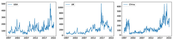
Figure 1.
Demonstrations of local EPU trends of UK, USA, and China.
For the empirical analysis in Section 4, we obtain the daily closing prices of gold futures from Wind (a widely used financial database in China, similar to Bloomberg) for the same time period as the EPU data. The statistical descriptions of these data will be provided in the corresponding section.
3. Methodology
3.1. PCA and Random Matrix Analysis
To write the local EPU of the i-th economy at time t as , we first normalize it to
where and denote the mean value and standard deviation of during the considered period. This step is necessary given the fact that EPU values of different countries may have been computed by different researchers which results in variations in dimension, and by normalizing, we can eliminate these potential discrepancies. Then, the normalized data from countries are arranged into the following () matrix X (called sample matrix for simplicity).
it is easily seen that is exactly the covariance matrix. Our purpose is to extract the dominant global pattern of all economies’ EPUs only through X, without referring to any other information such as GDP values. This task bears similarity to unsupervised machine learning, where a variety of algorithms are available. For this analysis, we employ the Principal Component Analysis (PCA), one of the most standard algorithms widely used in areas such as image compression. The PCA interprets the rows of X as a cloud of data points in a T-dimensional hyperspace and identifies principal components as mutually orthogonal directions along which the variances of the data points decrease monotonically. Mathematically, the PCA is executed by performing Singular Value Decomposition (SVD) on X, namely
where V is an matrix with non-zero diagonals denoting the singular values arranged in a decreasing order of magnitude. It can be readily observed that corresponds to the eigenvalues of the covariance matrix C. In PCA terminology, is referred to as the ’explained variance ratio’. By employing SVD, we decompose EPUs into orthonormal components —the k-th row of matrix W—each with weight . Each represents a specific global pattern of the EPUs. The columns of , or equivalently, the rows of U, illustrate interaction patterns among different economies. In most PCA applications, only the first few principal components with larger values are retained, thereby achieving dimension reduction (analogous to image compression). However, the criteria for retaining or discarding a component is not definitively established and often relies on the researcher’s experience. In this study, we adopt a concept from the random matrix theory to discern whether a component is random/trivial or non-trivial. The former should be discarded, while the latter should be retained.
The strategy is to assess how closely the sample matrix X approximates a composition of random time-series, or equivalently, how closely the covariance matrix approximates a matrix with random elements; this purpose can be achieved with the random matrix theory (RMT). The method of the random matrix theory originates from the physics society that dealt with complex nuclei in the 1960s, and has been brought to the analysis of economic and financial data in the last twenty years [36,37,38,39]. In short, the RMT offers a universal criteria to distinguish random information from non-random information in complex bid data; this task is normally accomplished by examining the probability distribution of —the eigenvalues of the covariance matrix– and comparing it to the theoretical prediction, where those eigenvalues that fall out of the RMT predicted range are non-random and contain non-trivial economical information [39]. However, this method usually requires a large amount of data and is thus inapplicable in this study. As an alternative, we directly inspect the scaling behavior of as a function of the component index k. Recent studies [40,41,42] suggest that if the sample matrix X consists of a randomly correlated series, then . Our numerical results for are depicted in Figure 2a. We can see that can be classified into three parts: (i) the dominant , which is significantly larger than the rest, indicating that is the only dominant feature of the EPUs—the principal component. (ii) For , the weights are so small that they contribute negligibly to the EPUs and can be neglected. (iii) For the intermediate range , follows a power-law (fractal) behavior , with . This implies that these principal components bear similarity to a random matrix pattern and contain random information; hence, they should be omitted.
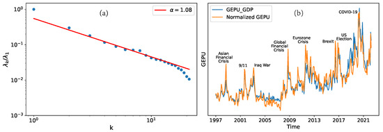
Figure 2.
(a) For the scaling behavior of , the majority part follows a power-law (fractal) function , meaning that they are close to a random matrix pattern. The dominant corresponds to the non-trivial principal component , which is thus proposed to be the NGEPU. (b) For the comparison between the normalized GEPU (NGEPU) and , both indices show local peaks around the periods of typical global events. For the eyes’ convenience, we have rescaled the two GEPUs to the same range.
From these observations, we conclude that the dominant component is the only non-trivial component in the sample matrix X that is non-random and of economic interest, and is thus a logical candidate for a new GEPU index. This implies that the dominant interaction pattern among economies is encoded in , where the elements of represent the weight of each economy’s EPU in constructing the GEPU, akin to the GDP of each economy in the construction of the GEPU index. The behavior of is illustrated in Figure 2b, where we also plot the index for comparison. As we can see, both indices can identify typical global events through their local maxima. In fact, displays more pronounced peaks around most local maxima.
At this stage, we have justified the fundamental requirements for to be a valid GEPU index, and given its unit norm, we term it the Normalized Global Economic Policy Uncertainty (NGEPU) index. This NGEPU differs from the one presented in Ref. [33], which is an un-normalized index.
Before proceeding, it is worth highlighting that the power-law behavior in the intermediate regime in Figure 2a is particularly significant in consideration of the limited size of the EPU data. In general, a random matrix analysis requires a large data size and careful evaluation to fully separate the random and non-trivial patterns of economical/financial data, as shown in, e.g., Ref. [39]. The outstanding efficiency in the EPU case reflects both the advantage of PCA and the intrinsic structure of EPUs.
3.2. Topological Characterizations Using Complex Networks
Before evaluating the efficacy of NGEPU in the empirical analysis, it is beneficial to perform a comparison between this new index and the traditional GEPU index. Since they have different scales, a direct statistical comparison is unsuitable. Instead, we will use methods from the complex network analysis to compare their topologies.
The techniques of the complex network analysis aim at converting time series into complex graphs using proper algorithms. Here, we utilize the Visibility Graph (VG) algorithm, whose construction proceeds as follows [43,44,45]. For a discrete time series , we represent them as consecutive data points in a two-dimensional space, known as vertices. Two vertices and are connected by an edge if the criterion
is fulfiled for all . The collection of all vertices— V, and all edges—E, constitutes a graph . Here, we focus on the simplest case where edges are unweighted and undirected. Evidently, in this context, all vertices are connected to their immediate neighbors. By transforming NGEPU and GEPU into VGs, we can compare their topologies independently of their scales.
In a VG, the most important characteristics are the degree and clustering coefficient statistics. The degree of a vertex——is the number of vertices connected with . Given the VG construction, we know that each vertex (except for the starting and ending points) is connected to at least its two neighbors, i.e., . In the VGs of the two GEPUs, we find that the ending points only connect to their neighboring vertex, while the starting points connect to at least one additional vertex besides their neighbors. Hence, we exclude the ending points when counting the VGs’ statistics.
The other quantity of interest is the clustering coefficient , defined as follows:
where is the number of edges between the vertices connected to vertex i. Clearly, the maximum value of is , implying . A high value of denotes a cluster centered around vertex i, which is the origin of its name.
We calculate the maximum, minimum, mean value, and standard deviation of in both VGs; the results are summarized in Table 1. We find that their statistics are qualitatively similar, reflecting the resemblance between them. The mean values of k and c— and —are roughly 9 and , respectively, indicating that the VGs are dense and the GEPUs are highly persistent in both cases.

Table 1.
The statistics of the VGs generated from two kinds of GEPU indices, show similar persistent behaviors, which is also reflected by the Hurst exponents.
Finally, the Hurst exponents of the GEPU indices are computed using the R/S method. The Hurst exponent is a common tool to measure the long-term memory of a time series, which is dimensionless and takes on values between 0 and 1. In our case, the computed Hurst exponent values for the NGEPU and GEPU are and , respectively, with both of them significantly larger than , indicating that the GEPU indices exhibit a strong persistence, which means that high values are likely to be followed by high values and low values by low values. This result aligns with the previous VG analysis, which suggests a long memory property in both indices and supports the NGEPU as a valid index for characterizing global economic policy uncertainty.
4. Empirical Analysis
In this section, we seek to elucidate the merits of the newly introduced NGEPU index in the context of empirical financial market studies, with a particular focus on the volatility of gold’s future prices. The foundation for our investigation lies in the GARCH-MIDAS (MIxed DAta Sampling) model, as originally proposed by Engle [46]. This efficient model incorporates economical data that are sampled at different frequencies, for instance, the gold future prices observed on a daily frequency, and the EPU index that is sampled monthly. The GARCH-MIDAS model decomposes the volatility of the gold future price into two components: high-frequency (daily) volatility and low-frequency (monthly) volatility. The high-frequency component is dictated by the inherent dynamics of the time series, whereas the low-frequency volatility is characterized by the realized volatility (RV) and a macroeconomic variable, namely the GEPU. The mathematical formulation goes as follows.
Write the logarithmic future price return at day i in month t as ; the GARCH-MIDAS assumes into the following form:
The conditional variance is thus
where is the low-frequency (monthly) fluctuation, and is the high-frequency (daily) fluctuation. The is assumed to follow a GARCH(1,1) process that
where and . The long-term variance is specified by smoothing the realized volatility (RV) and GEPU differences through MIDAS regression, that is
where
is the realized volatility in month t, and denotes the number of trading days in this month, which is set to be for convenience. The weighting function in the above model is the so called Beta weights defined as
which satisfies . The GARCH-MIDAS model is thus defined through Equations (7)–(12) over the parameter space . Among them, and will be our primary interests.
Using the GARCH-MIDAS model, Fang [32] established the theoretical foundation for a positive correlation between the volatility of gold future price returns and GEPU. In short, gold plays the role of a safe-haven asset during periods of market turmoil when the volatile macroeconomic policy environment is indicated by a high value of EPU. This environment undermines investor confidence, precipitating a concurrent steep decline in the stock markets. In contrast, the allure of gold investment amplifies its current volatility, subsequently elevating future volatility. Here, we aim to perform a comparative study to verify the efficiency of the proposed NGEPU index.
For our purpose, we collect the daily closing prices of gold futures from the Wind software, with a time range from 2 January 1998 to 29 April 2022. Table 2 displays the statistics of the data we used, where we computed the minimum, maximum, mean value, standard error, skewedness, and kurtosis of the considered series. It is noteworthy that the distributions of the future price returns are negatively skewed, while those of GEPU variations display positive skewedness, and both of them are leptokurtic. Additionally, we confirm their stationarity via the augmented Dickey–Fuller (ADF) test, ensuring their appropriateness for modeling using the GARCH-MIDAS model.
Table 2.
Statistics of the gold future price returns, as well as the GEPU and NGEPU changes. ADF is the statistics calculated from the unit root test, and denotes that the significance level is at the 1% level.
Then, we perform the GARCH-MIDAS simulation for the volatilities of gold futures and GEPU. We first employed the conventional GEPU index. The simulation results are presented in Table 3; the results (fitted values and significance levels) we obtained are very similar to Ref. [32]. Since the time period we consider is different from Ref. [32] (which does not contain the COVID-19 period after 2019), our simulation can serve as a robustness test for the considered model.
Table 3.
Left panel: The estimates of the GARCH-MIDAS coefficients using two kinds of GEPU indices. The data covers daily closing prices from 2 January 1998 to 29 April 2022. : Significance at the 1% level; significance at the 5% level. Numbers in parentheses are the standard deviations. Right panel: The loss functions for out-of-sample volatility forecast using two GEPU indices.
Next, we perform the same simulation using the new NGEPU index; the results are also in Table 3. As expected, stays positive, confirming the positive impact of NGEPU on the gold future price volatility. Actually, the significance level for and (both at the 1% level) are both higher than those in the GEPU case (5% and 10% for and , respectively). This illustrates the superiority of the NGEPU index, that is, it eliminates potential endogeneity prompted by GDP in GEPU and hence, behaves better in empirical studies.
As a final step, as the central goal of the GARCH-type model is to make volatility forecasting, we examine the predictive ability of the GARCH-MIDAS model for gold future price returns, with the aim to discern whether the new NGEPU index outperforms GEPU. Specifically, we carry out in-sample estimations of the GARCH-MIDAS models for the period 1998–2019, then utilize the estimated parameters to make out-of-sample forecasts for the period 2020–2022. To evaluate the accuracy of these predictions, we employ four standard loss functions: RMSE (Root Mean Square Error), RMAD (Root Mean Absolute Deviation), MSPE (Mean Square Percentage Error), and MAPE (Mean Absolute Percentage Error). Given that the in-sample estimations of the GARCH-MIDAS models are akin to those for the whole sample, we only provide the loss function values for out-of-sample forecasts, which appear in the right panel of Table 3. It is evident that the loss functions with the NGEPU are generally lower than with GEPU, with the most significant difference observable in the MAPE measure. This underscores the efficiency of the NGEPU in terms of its forecasting ability, which, combined with the previously discussed results, confirms the NGEPU as a suitable GEPU index.
5. Conclusions and Discussion
In this work, we proposed a normalized global EPU (NGEPU) index from the unsupervised machine learning algorithm—principal component analysis (PCA). The primary contributions of this work can be summarized as follows.
First of all, from a mathematical perspective, we brought the latest developments of the random matrix theory into the conventional PCA, and point out that the former can distinguish the random (trivial) components from the non-random components that contain nontrivial economic information. A prominent illustration of this is the proposed NGEPU index, which does not rely on extra economic data except for the EPUs themselves. It is crucial to highlight that this synthesis of the random matrix theory and PCA constitutes a natural algorithm, whose practical efficiency and mathematical rigor make it highly adaptable to related scenarios, even those with relatively smaller datasets.
Secondly, from an economic point of view, we validated the effectiveness of the NGEPU index in identifying typical global events from its local peaks, in a similar manner to the commonly used index. However, the NGEPU index does not depend on GDP values, thereby circumventing the potential endogeneity introduced by the latter. Consequently, the NGEPU demonstrates better performance over in empirical studies about the future price volatility with the GARCH-MIDAS model. This underscores the importance of further implementing the NGEPU index in various scenarios. Needless to say, to fully reveal the advantage of this new index, more empirical studies are required, which goes beyond the scope of the current study and will be presented in future works. In fact, the construction of the NGEPU index allows for an empirical study between GEPU and GDP itself—a fascinating direction that warrants future exploration.
Last but not least, we employed the cross-sectional algorithm—the visibility graph (VG) algorithm—to compare the NGEPU and . The VG algorithm enables topological characterizations of GEPUs that are independent of scales, and the results confirm that both of them are highly persistent, consistent with the Hurst indices. The VG algorithm, as well as many other methodologies from complex networks and the aforementioned random matrix theory, offer valuable additions to traditional econometric tools from the interdisciplinary perspective, aiding the exploration and understanding of economic phenomena.
Author Contributions
Conceptualization: W.R., L.W. and Q.W.; Data curation: W.X. and W.R.; Methodology, W.X. and W.R.; Visualization, writing draft: W.X., W.R. and Q.W.; Review and editing, Q.W. and L.W. All authors have read and agreed to the published version of the manuscript.
Funding
W. Rao is supported by the Zhejiang Provincial Natural Science Foundation of China under Grant No.LY23A050003, and L. Wei is supported by the Major Project of National Social Science Fund of China (22&ZD081) and the National Natural Science Foundation of China (71972123).
Data Availability Statement
The data sets used and/or analyzed during the current study are available from the corresponding author on reasonable request.
Conflicts of Interest
The authors declare no conflict of interest.
References
- Baker, S.R.; Bloom, N.; Davis, S.J. Measuring Economic Policy Uncertainty. NBER Work. Pap. 2013, 21633. Available online: abfer.org/media/abfer-events-2013/annual-conference/corporate-finance/track2-presentation-measuring-economic-policy-uncertainty.pdf (accessed on 19 July 2023). [CrossRef]
- Baker, S.R.; Bloom, N.; Davis, S.J. Measuring economic policy uncertainty. Quart. J. Econ. 2016, 131, 1593–1636. [Google Scholar] [CrossRef]
- Saxegaard, E.C.A.; Davis, S.J.; Ito, A.; Miake, N.; Saito, I. Policy Uncertainty in Japan. J. Jpn. Int. Econ. 2022, 64, 101192. [Google Scholar] [CrossRef]
- Baker, S.R.; Bloom, N.; Davis, S.J.; Wang, X.X. Economic Policy Uncertainty in China. Unpublished Paper; University of Chicago: Chicago, IL, USA, 2013. [Google Scholar]
- Ghirelli, C.; Perez, J.J.; Urtasun, A. A new economic policy uncertainty index for Spain. Econ. Lett. 2019, 182, 64–67. [Google Scholar] [CrossRef]
- Moore, A. Measuring economic uncertainty and its effects. Econ. Rec. 2017, 93, 550–575. [Google Scholar] [CrossRef]
- Kloßner, S.; Sekkel, R. International spillovers of policy uncertainty. Econ. Lett. 2014, 124, 508–512. [Google Scholar] [CrossRef]
- Yeşiltaş, S.; Şen, A.; Arslan, B.; Altuǧ, S. A twitter-based economic policy uncertainty index: Expert opinion and financial market dynamics in an emerging market economy. Front. Phys. 2021, 10, 864207. [Google Scholar] [CrossRef]
- Lu, X.; Lang, Q. Categorial economic policy uncertainty indices or Twitter-based uncertainty indices? Evidence from Chinese stock market. Financ. Res. Lett. 2023, 55, 103936. [Google Scholar] [CrossRef]
- Miranda-Belmonte, H.U.; Muñiz-Sánchez, V.; Corona, F. Word embeddings for topic modeling: An application to the estimation of the economic policy uncertainty index. Expert Syst. Appl. 2023, 211, 118499. [Google Scholar] [CrossRef]
- Davis, S.J. An Index of Global Economic Policy Uncertainty; Technical Report; NBER Working Paper No. 22740; NBER: Cambridge, MA, USA, 2016. [Google Scholar]
- Li, X.M.; Zhang, B.; Gao, R. Economic policy uncertainty shocks and stock-bond correlations: Evidence from the US market. Econ. Lett. 2015, 132, 91–96. [Google Scholar] [CrossRef]
- Brogaard, J.; Detzel, A. The asset-pricing implications of government economic policy uncertainty. Manag. Sci. 2015, 61, C3–C18. [Google Scholar] [CrossRef]
- Hoque, M.E.; Zaidi, M.A.S. The Impacts of Global Economic Policy Uncertainty on Stock Market Returns in Regime Switching Environment: Evidence from Sectoral Perspectives. Int. J. Financ. Econ. 2019, 24, 991–1016. [Google Scholar] [CrossRef]
- Balcilar, M.; Gupta, R.; Kyei, C.; Wohar, M.E. Does Economic Policy Uncertainty Predict Exchange Rate Returns and Volatility? Evidence from a Nonparametric Causality-in-quantiles Test. Open Econ. Rev. 2016, 27, 229–250. [Google Scholar] [CrossRef]
- Shahabad, R.D.; Balcilar, M. Modelling the dynamic interaction between economic policy uncertainty and commodity prices in India: The dynamic autoregressive distributed lag approach. Mathematics 2022, 10, 1638. [Google Scholar] [CrossRef]
- Pástor, L. Veronesi Uncertainty about government policy and stock prices. J. Financ. 2012, 67, 1219–1264. [Google Scholar] [CrossRef]
- Pástor, L. Veronesi Political uncertainty and risk premia. J. Financ. Econ. 2013, 110, 520–545. [Google Scholar] [CrossRef]
- Ersan, O.; Akron, S.; Demir, E. The effect of European and global uncertainty on stock returns of travel and leisure companies. Tour. Econ. 2019, 25, 51–66. [Google Scholar] [CrossRef]
- Berger, T.; Uddin, G.S. On the Dynamic Dependence Between Equity Markets, Commodity Futures and Economic Uncertainty Indexes. Energy Econ. 2016, 56, C374–C383. [Google Scholar] [CrossRef]
- He, H.Z.; Sun, M.; Gao, C.X.; Li, X.M. Detecting lag linkage effect between economic policy uncertainty and crude oil price: A multi-scale perspective. Physica A 2021, 580, 126146. [Google Scholar] [CrossRef]
- Dai, P.F.; Xiong, X.; Zhang, J.; Zhou, W.X. The role of global economic policy uncertainty in predicting crude oil futures volatility: Evidence from a two-factor GARCH-MIDAS model. Resour. Policy Resour. Policy 2022, 78, 102849. [Google Scholar] [CrossRef]
- Lyu, Y.J.; Tuo, S.W.; Wei, Y.; Yang, M. Time-varying effects of global economic policy uncertainty shocks on crude oil price volatility: New evidence. Resour. Policy 2021, 70, 101943. [Google Scholar] [CrossRef]
- Yi, A.; Yang, M.L.; Li, Y.S. Macroeconomic Uncertainty and Crude Oil Futures Volatility-Evidence from China Crude Oil Futures Market. Front. Environ. Sci. 2021, 9, 636903. [Google Scholar] [CrossRef]
- Yang, L. Connectedness of economic policy uncertainty and oil price shocks in a time domain perspective. Energy Econ. 2019, 80, 219–233. [Google Scholar] [CrossRef]
- Zhao, L. Global economic policy uncertainty and oil futures volatility prediction. Financ. Res. Lett. 2023, 54, 103693. [Google Scholar] [CrossRef]
- Lyu, Y.J.; Yi, H.L.; Hu, Y.Y.; Yang, M. Economic uncertainty shocks and China’s commodity futures returns: A time-varying perspective. Resour. Policy 2021, 70, 101979. [Google Scholar] [CrossRef]
- Ma, F.; Lu, X.; Wang, L.; Chevallier, J. Global economic policy uncertainty and gold futures market volatility: Evidence from Markov regime-switching GARCH-MIDAS models. J. Forecast. 2021, 40, 1070–1085. [Google Scholar] [CrossRef]
- Xu, Y.; Wang, X.Y.; Liu, H.N. Quantile-based GARCH-MIDAS: Estimating value-at-risk using mixed-frequency information. Financ. Res. Lett. 2021, 43, 101965. [Google Scholar] [CrossRef]
- Liu, J.; Zhang, Z.T.; Yan, L.Z.; Wen, F.H. Forecasting the volatility of EUA futures with economic policy uncertainty using the GARCH-MIDAS model. Financ. Innov. 2021, 7, 1–19. [Google Scholar] [CrossRef]
- Xiao, X.Y.; Tian, Q.S.; Hou, S.X.; Li, C.G. Economic policy uncertainty and grain futures price volatility: Evidence from China. China Agric. Econ. Rev. 2019, 11, 642–654. [Google Scholar] [CrossRef]
- Fang, L.; Chen, B.; Yu, H.; Qian, Y. The importance of global economic policy uncertainty in predicting gold futures market volatility: A GARCH-MIDAS approach. J. Futur. Mark. 2018, 38, 413–422. [Google Scholar] [CrossRef]
- Dai, P.F.; Xiong, X.; Zhou, W.X. A global economic policy uncertainty index from principal component analysis. Financ. Res. Lett. 2021, 40, 101686. [Google Scholar] [CrossRef]
- Libório, M.; Martinuci, O.D.; Machado, A.M.C.; Hadad, R.; Bernardes, P.; Camacho, V.A.L. Adequacy and Consistency of an Intraurban Inequality Indicator Constructed through Principal Component Analysis. Prof. Geogr. 2021, 73, 282–296. [Google Scholar] [CrossRef]
- Mazziotta, M.; Pareto, A. Use and Misuse of PCA for Measuring Well-Being. Soc. Indic. Res. 2019, 142, C451–C476. [Google Scholar] [CrossRef]
- Bhosale, U.T.; Tekur, S.H.; Santhanam, M.S. Scaling in the eigenvalue fuctuations of correlation matrices. Phys. Rev. E 2018, 98, 052133. [Google Scholar] [CrossRef]
- Laloux, L.; Cizeau, P.; Bouchaud, J.-P.; Potters, M. Noise dressing of fnancial correlation matrices. Phys. Rev. Lett. 1999, 83, 1467. [Google Scholar] [CrossRef]
- Plerou, V.; Gopikrishnan, P.; Rosenow, B.; Amaral, L.A.N.; Stanley, H.E. Universal and nonuniversal properties of cross correlations in fnancial time series. Phys. Rev. Lett. 1999, 83, 1471. [Google Scholar] [CrossRef]
- Plerou, V.; Gopikrishnan, P.; Rosenow, B.; Amaral, L.A.N.; Guhr, T.; Stanley, H.E. Random matrix approach to cross correlations in fnancial data. Phys. Rev. E 2002, 65, 066126. [Google Scholar] [CrossRef]
- Relanõ, A.; Gómez, J.M.G.; Molina, R.A.; Retamosa, J.; Faleiro, E. Quantum Chaos and 1/f Noise. Phys. Rev. Lett. 2002, 89, 244102. [Google Scholar] [CrossRef]
- Faleiro, E.; Gómez, J.M.G.; Molina, R.A.; Muñoz, L.; Relanõ, A.; Retamosa, J. Theoretical Derivation of 1/f Noise in Quantum Chaos. Phys. Rev. Lett. 2004, 93, 244101. [Google Scholar] [CrossRef]
- Fossion, R.; Torres Vargas, G.; Lopez Vieyra, J.C. Random-matrix spectra as a time series. Phys. Rev. E 2013, 88, 060902. [Google Scholar] [CrossRef]
- Zhang, J.; Small, M. Complex network from pseudoperiodic time series: Topology versus dynamics. Phys. Rev. Lett. 2006, 96, 238701. [Google Scholar] [CrossRef] [PubMed]
- Dai, P.F.; Xiong, X.; Zhou, W.X. Visibility graph analysis of economy policy uncertainty indices. Physica A 2019, 10, 0378–4371. [Google Scholar] [CrossRef]
- Zou, Y.; Donner, R.V.; Marwan, N.; Donges, J.F.; Kurths, J. Complex network approaches to nonlinear time series analysis. Phys. Rep. 2019, 787, 1–97. [Google Scholar] [CrossRef]
- Engle, R.F.; Ghysels, E.; Sohn, B. Stock market volatility and macroeconomic fundamentals. Rev. Econ. Stat. 2013, 95, 776–797. [Google Scholar] [CrossRef]


Disclaimer/Publisher’s Note: The statements, opinions and data contained in all publications are solely those of the individual author(s) and contributor(s) and not of MDPI and/or the editor(s). MDPI and/or the editor(s) disclaim responsibility for any injury to people or property resulting from any ideas, methods, instructions or products referred to in the content. |
© 2023 by the authors. Licensee MDPI, Basel, Switzerland. This article is an open access article distributed under the terms and conditions of the Creative Commons Attribution (CC BY) license (https://creativecommons.org/licenses/by/4.0/).