

Research on Real-Time Detection Algorithm for Pavement Cracks Based on SparseInst-CDSM
Abstract
:1. Introduction
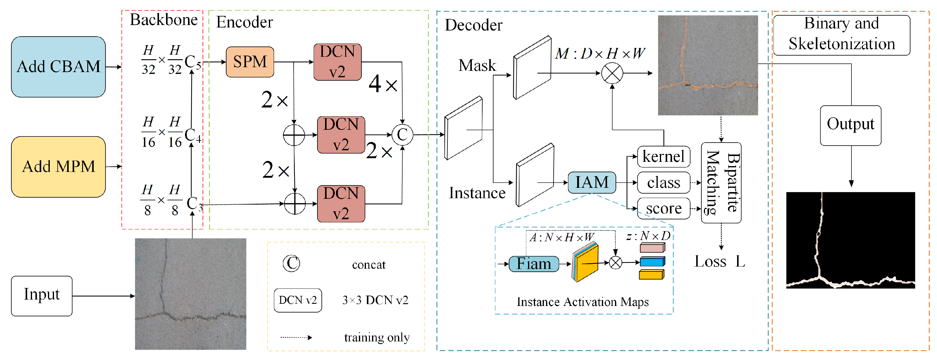
2. Methodology
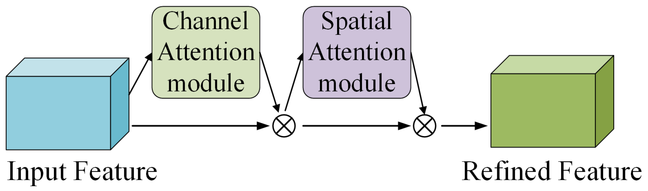
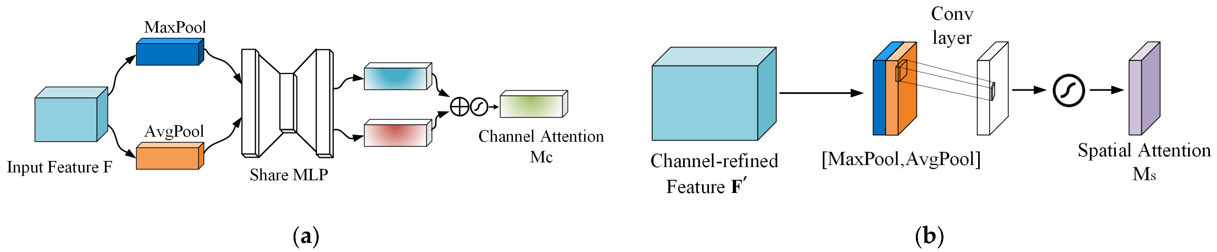
2.1. Attention Mechanism Module
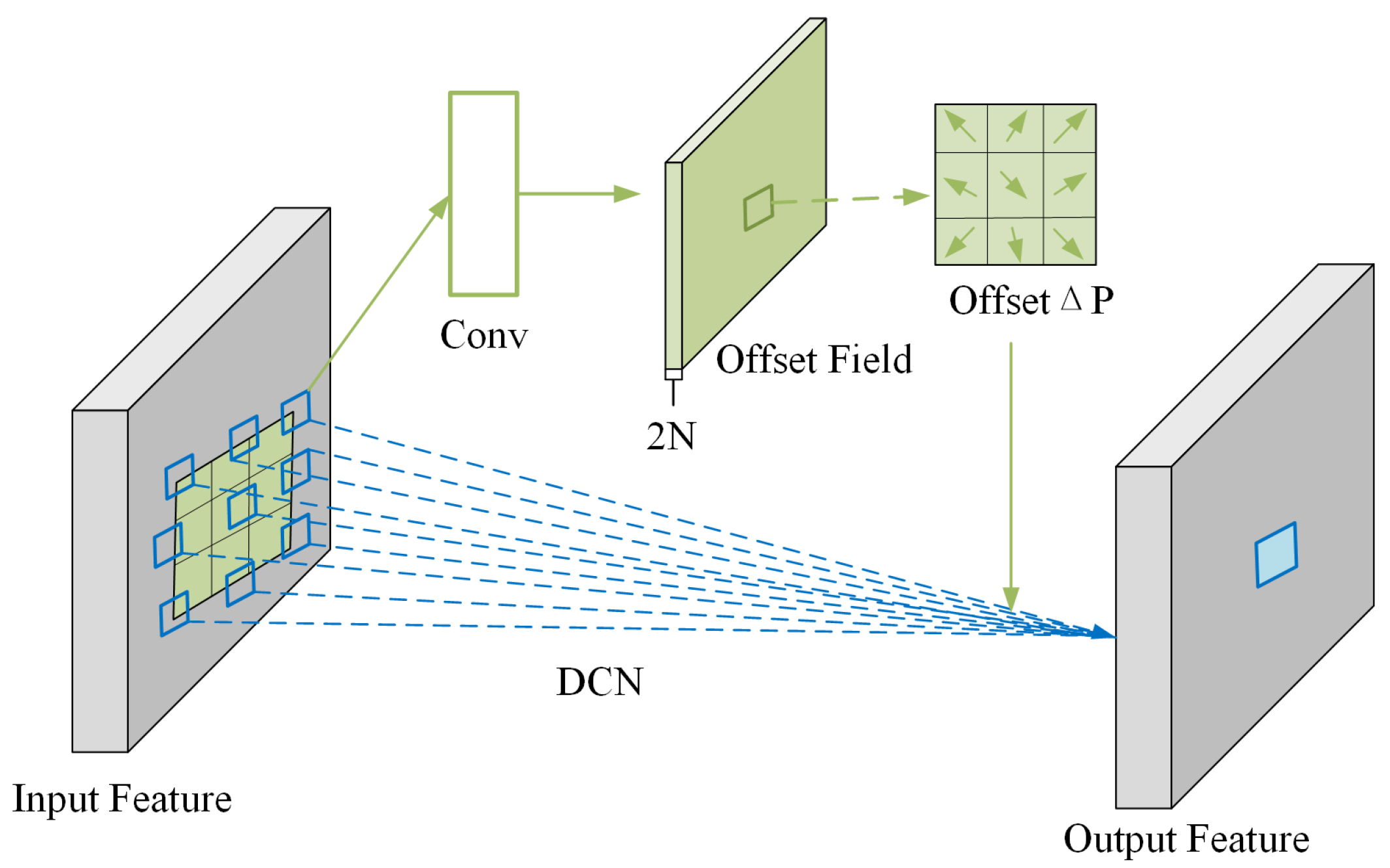
2.2. Deformable Convolution Module
2.3. Improved Context Encoder
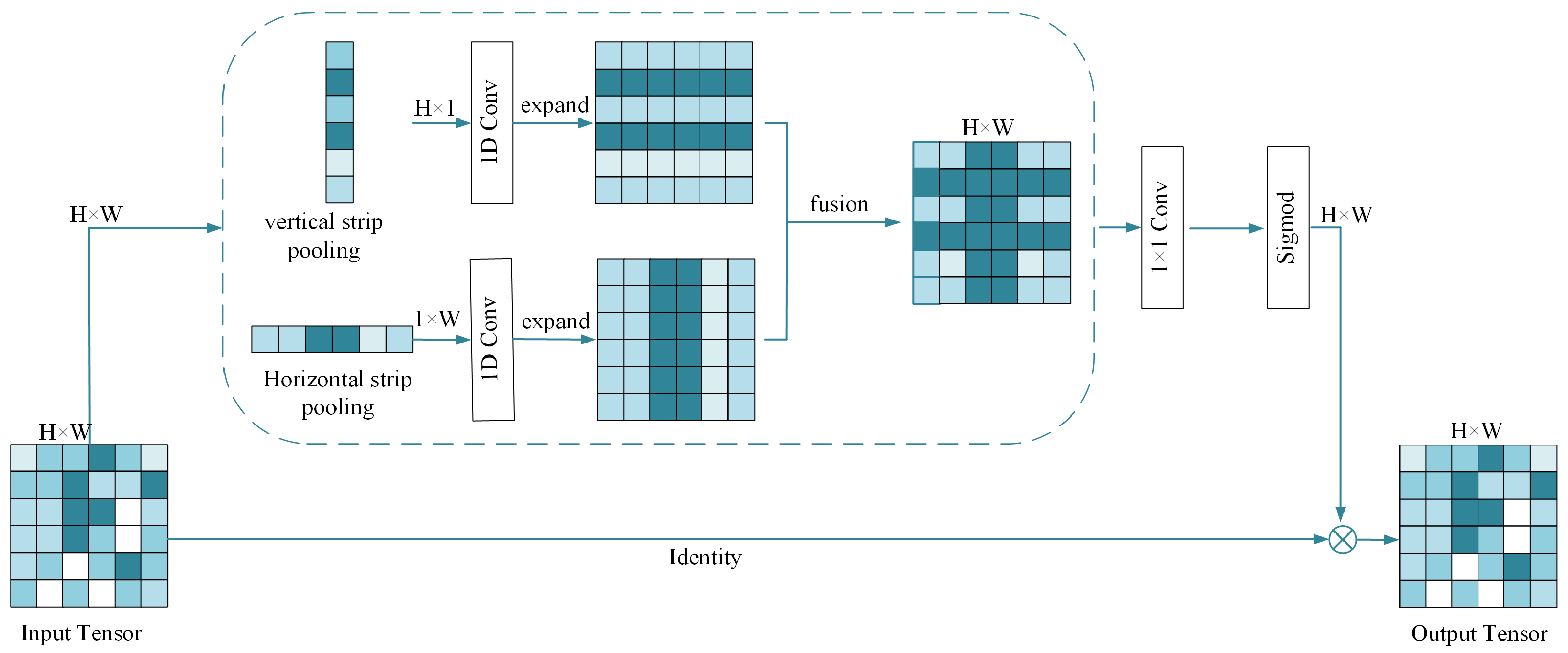
2.4. Add Mix Pooling Module
2.5. Preventing the Problem of Overfitting
- (1)
- Data Augmentation: By randomly transforming and augmenting the training data, the diversity of the training data can be increased. This can effectively reduce overfitting and improve the model’s generalization to new images. The data augmentation operations used in this paper include random cropping, rotation, scaling, and flipping.
- (2)
- Regularization: Regularization is a method of limiting the complexity of the model by introducing a regularization term into the loss function. Common regularization methods include L1 regularization and L2 regularization. In this paper, regularization is used to penalize large weight values in the model, thereby avoiding overfitting.
- (3)
- Early Stopping: Early stopping is a simple and effective method to prevent overfitting. It monitors the performance metrics on the validation set and stops training before the model starts to overfit. Generally, when the performance on the validation set no longer improves, it can be considered that the model has reached its best generalization ability.
3. Crack Skeleton Extraction and Crack Size Calculation
3.1. Crack Morphology Skeletonization
- (1)
- Convert the crack image into a binary image; that is, set the pixel values in the crack area of the image to white and other areas to black.
- (2)
- Use the Canny algorithm [47] to perform edge detection on the binary image.
- (3)
- The skeletonization algorithm proposed by Ma et al. [48] is used to skeletonize the binary image obtained by edge detection and extract the midline of the crack area.
- (4)
- Connect the pixels on the medial axis to obtain the skeleton diagram of the crack.
- (5)
- Post-process the crack skeleton diagram to remove redundant lines and fill in broken line segments.
- (1)
- Because the duration of a curved crack should be significantly larger than its breadth, the maximum crack width specified in the precise crack quantification method of AASHTO PP67-10 is employed as the default cutoff for trimming [49].
- (2)
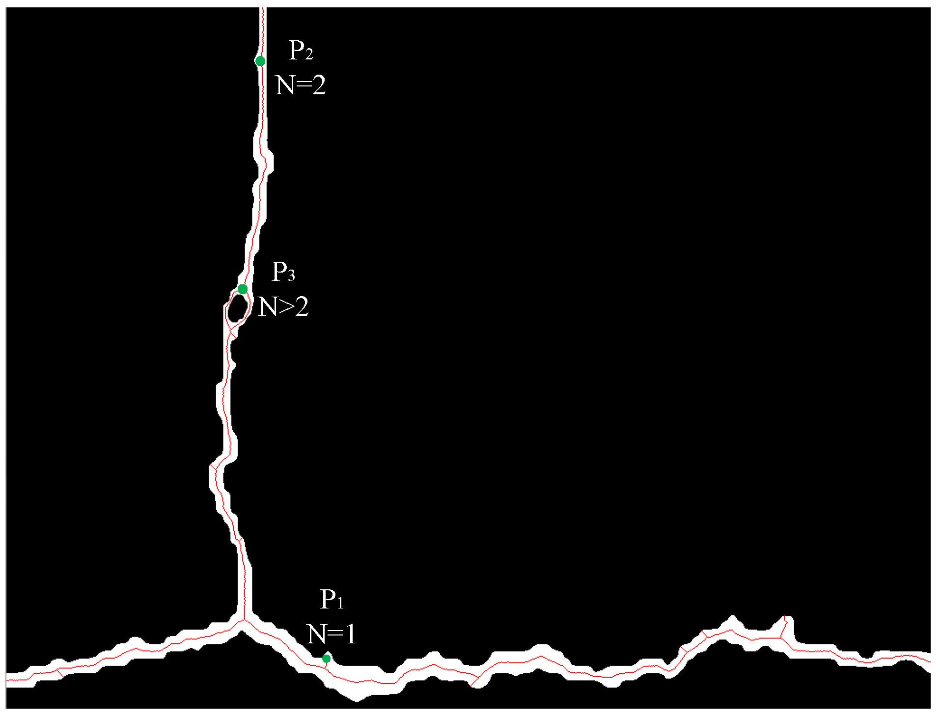
- Track the eight neighbors of each skeletal pixel in a clockwise fashion. Let N stand for how many times a pixel’s color switches from white to black. According to Figure 10, if N = 2, it is a typical skeletal pixel (P2); if N > 2, it is identified as an intersection (P3); if N = 1, the current pixel is an endpoint (P1).
- (3)
- Begin at any endpoint and work your way along the skeleton until you reach another endpoint or intersection; then, part of the skeleton is documented. The skeleton must be pruned if its length is less than the standard pruning threshold since it is redundantly short. After pruning, a result will be obtained, as shown in Figure 10.

3.2. Calculation of Crack Pixel Length
- (1)
- Using the total length calculation method, add the length of the main crack and its branch cracks to obtain the total length of the crack.
- (2)
- Using the main crack length calculation method, only calculate the length of the main crack and do not calculate the length of the branch cracks. This method is suitable for situations where the branch cracks are short and dense.
- (1)
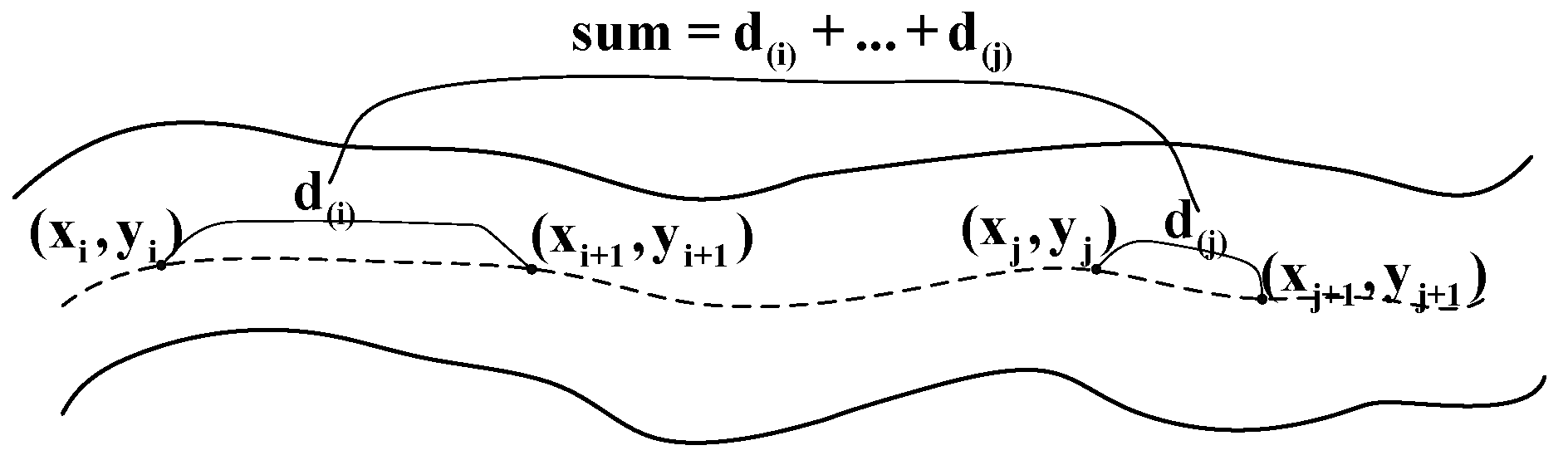
- Obtain the n sets of target point coordinates between the starting point and the end point through iterative branch skeleton.
- (2)
- Use the formula below to determine the straight-line separation between two places:
- (3)
- Include the line of sight distances of each part:
- (4)
- Keep repeating the above steps until the distance between the two points is finally calculated.
3.3. Calculation of Maximum Crack Pixel Width
- (1)
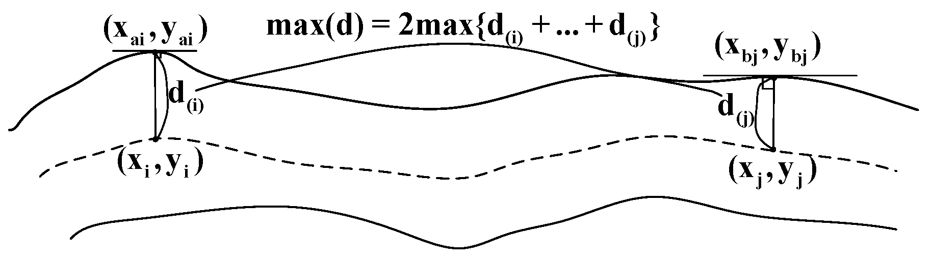
- Obtain the n sets of target point coordinates between the starting point and the endpoint through an iterative branch skeleton.
- (2)
- The orientation of the skeleton can be obtained from the coordinates of each point on the skeleton; that is, its normality is discernible. The appropriate points on the central axis can be identified by using the procedure described above to obtain their coordinates. The target point is (
- (3)
- The crack’s breadth is now equal to double the separation between the two points:
- (4)
- The largest crack at each point is compared:
- (5)
- Repeat the procedure a few more times to determine the last point’s crack’s breadth.
3.4. Calculation of Crack Physical Size
4. Experimental Results and Analysis
4.1. Experimental Environment
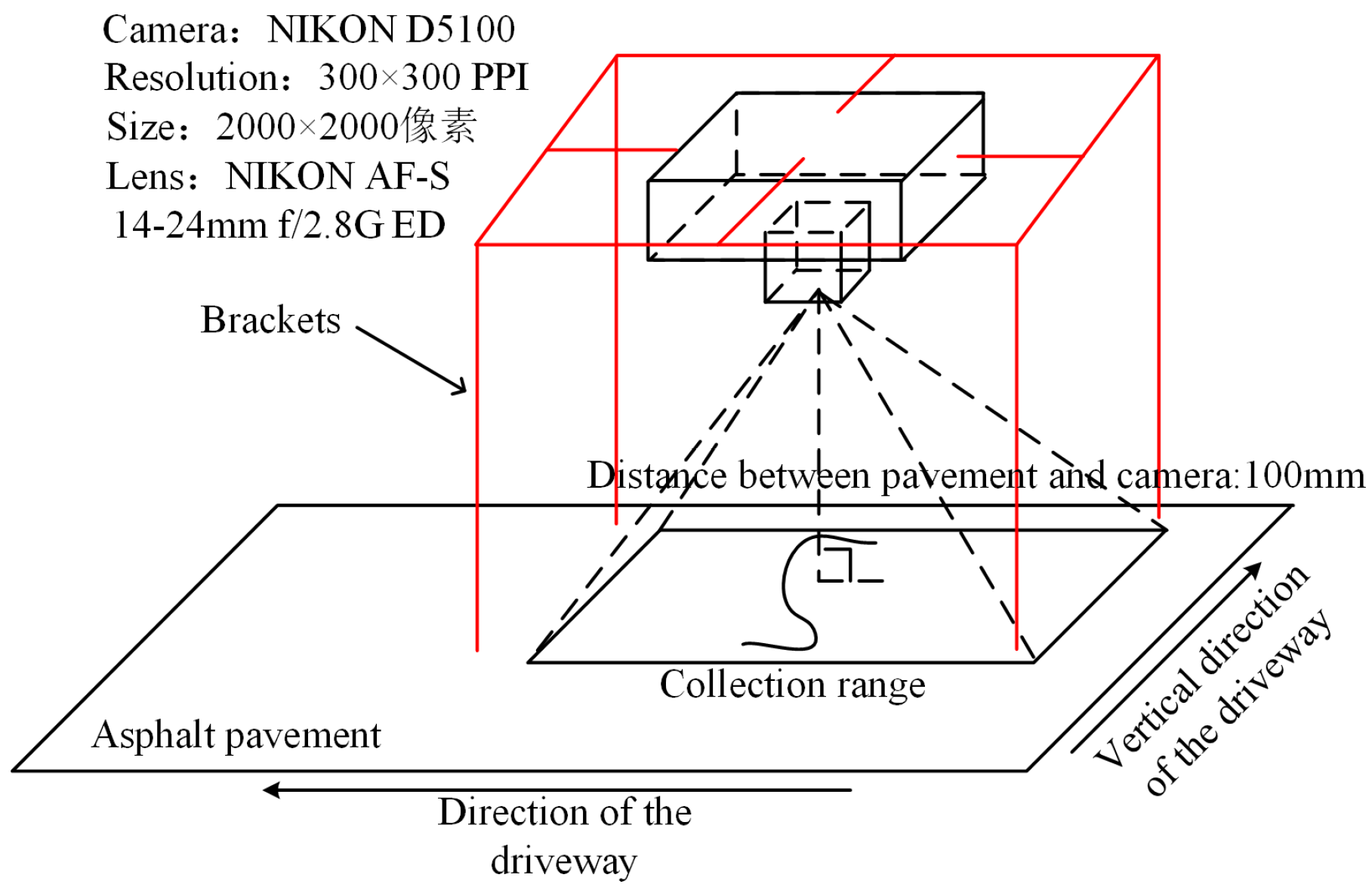
4.2. Experimental Dataset Collection
4.3. Set Evaluation Indicators
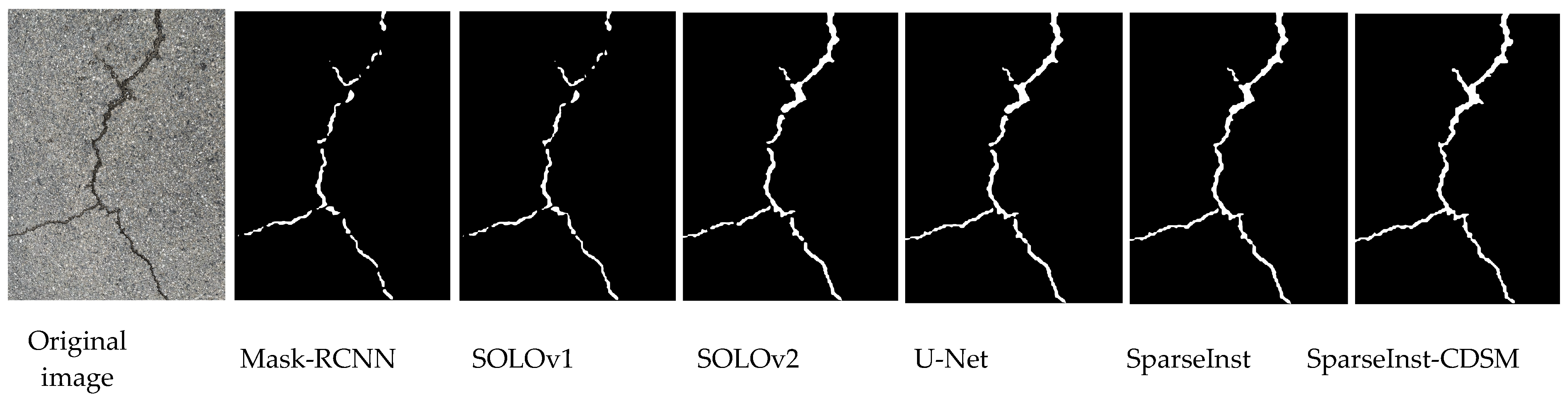
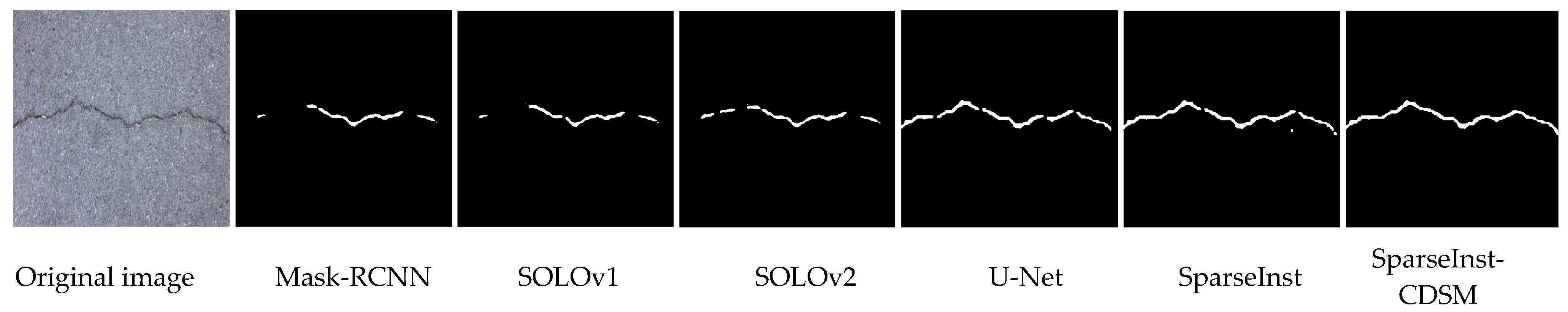
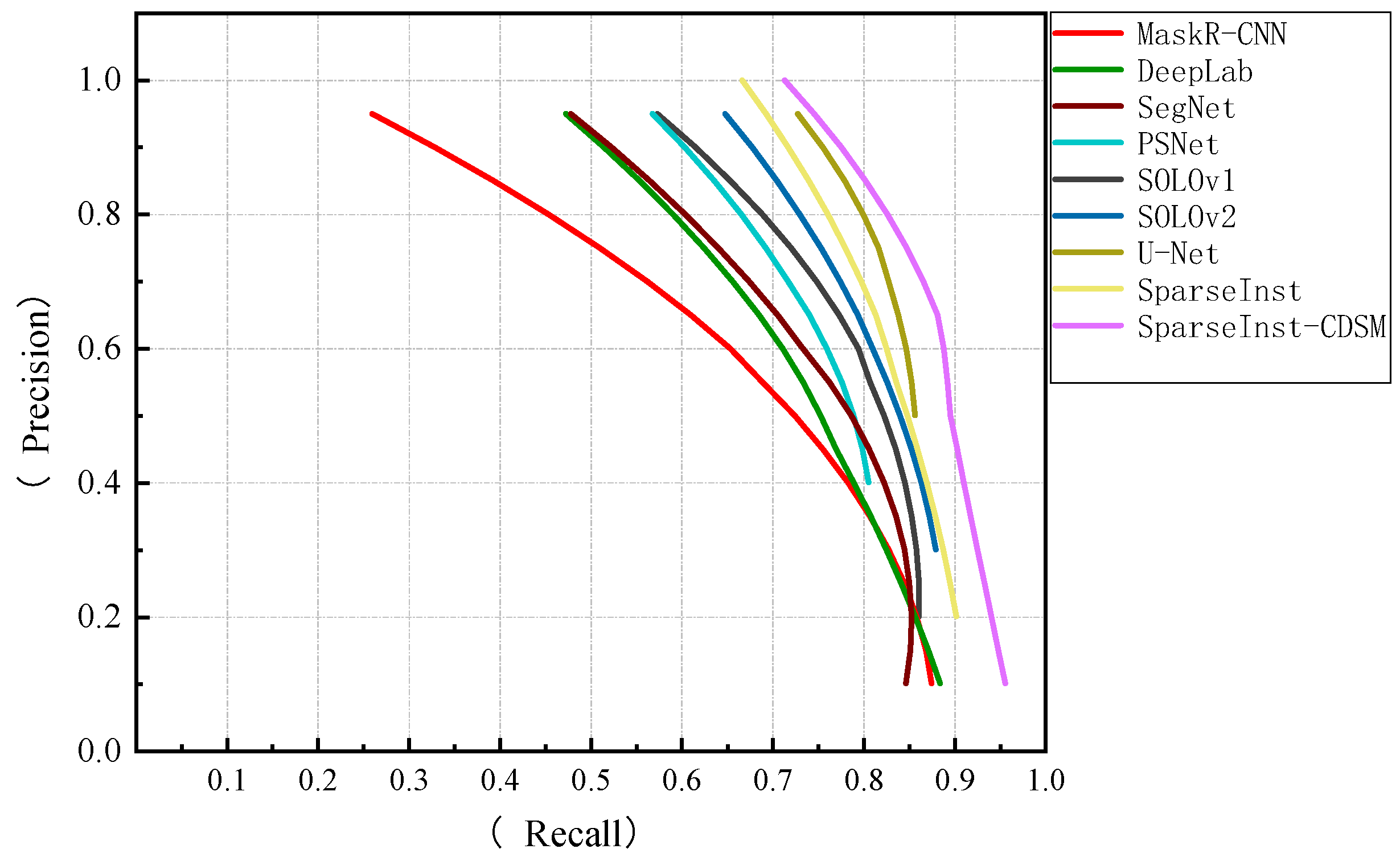
4.4. Instance Segmentation Comparison Experiment
4.5. Ablation Experiment
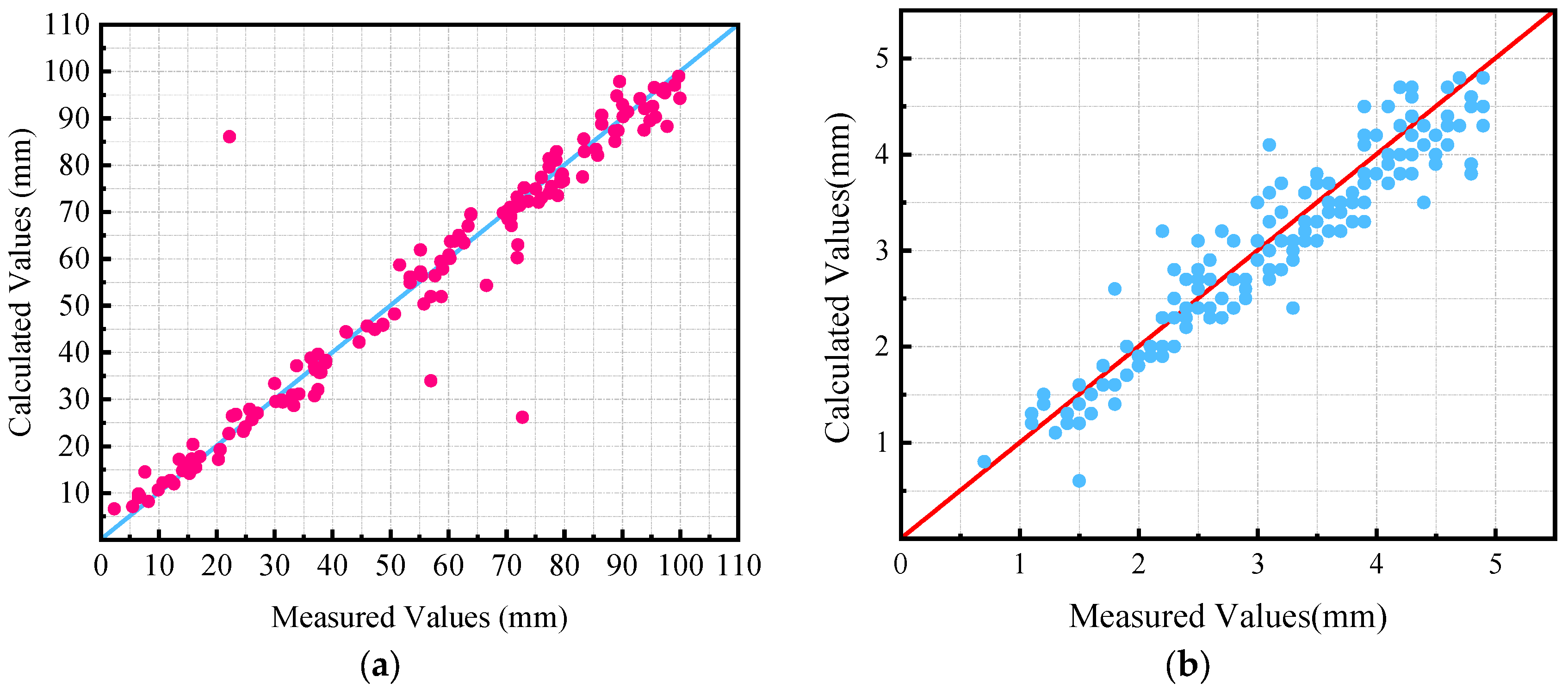
4.6. Comparison of Calculated and Measured Values of Cracks
5. Conclusions
Author Contributions
Funding
Data Availability Statement
Conflicts of Interest
References
- Gavilán, M.; Balcones, D.; Marcos, O.; Llorca, D.F.; Sotelo, M.A.; Parra, I.; Ocaña, M.; Aliseda, P.; Yarza, P.; Amírola, A. Adaptive Road Crack Detection System by Pavement Classification. Sensors 2011, 11, 9628–9657. [Google Scholar] [CrossRef] [PubMed]
- Sun, X.; Huang, J.; Liu, W. Decision model in the laser scanning system for pavement crack detection. Opt. Eng. 2011, 50, 127207. [Google Scholar] [CrossRef]
- Yao, M.; Zhao, Z.; Yao, X.; Xu, B. Fusing complementary images for pavement cracking measurements. Meas. Sci. Technol. 2015, 26, 025005. [Google Scholar] [CrossRef]
- Hu, G.X.; Hu, B.L.; Yang, Z.; Huang, L.; Li, P. Pavement Crack Detection Method Based on Deep Learning Models. Wirel. Commun. Mob. Comput. 2021, 2021, 1–13. [Google Scholar] [CrossRef]
- Abdellatif, M.; Peel, H.; Cohn, A.G.; Fuentes, R. Pavement Crack Detection from Hyperspectral Images Using A Novel Asphalt Crack Index. Remote Sens. 2020, 12, 3084. [Google Scholar] [CrossRef]
- Ren, J.; Zhao, G.; Ma, Y.; Zhao, D.; Liu, T.; Yan, J. Automatic Pavement Crack Detection Fusing Attention Mechanism. Electronics 2022, 11, 3622. [Google Scholar] [CrossRef]
- Wang, W.; Wu, L. Pavement crack extraction based on fractional integral valley bottom boundary detection. J. South China Univ. Technol. (Nat. Sci. Ed.) 2014, 42, 117–122. [Google Scholar]
- Liang, R.; Zhigang, X.; Xiangmo, Z.; Jingmei, Z. Pavement crack connection algorithm based on prim minimum spanning tree. Comput. Eng. 2015, 41, 31–36. [Google Scholar]
- Kirschke, K.R.; Velinsky, S.A. Histogram-based approach for automated pavement-crack sensing. J. Transp. Eng. 1992, 118, 700–710. [Google Scholar] [CrossRef]
- Oh, H.; Garrick, N.W.; Achenie, L.E. Segmentation algorithm using iterative clipping for processing noisy pavement images. In Imaging Technologies: Techniques and Applications in Civil Engineering. Second International Conference Engineering Foundation and Imaging Technologies Committee of the Technical Council on Computer Practices; American Society of Civil Engineers: Reston, VA, USA, 1998. [Google Scholar]
- Fang, C.; Zhe, L.; Li, Y. Images crack detection technology based on improved K-means algorithm. J. Multimed. 2014, 9, 822. [Google Scholar]
- Mathavan, S.; Vaheesan, K.; Kumar, A.; Chandrakumar, C.; Kamal, K.; Rahman, M.; Stonecliffe-Jones, M. Detection of pavement cracks using tiled fuzzy Hough transform. J. Electron. Imaging 2017, 26, 053008. [Google Scholar] [CrossRef] [Green Version]
- Amhaz, R.; Chambon, S.; Idier, J.; Baltazart, V. Automatic Crack Detection on Two-Dimensional Pavement Images: An Algorithm Based on Minimal Path Selection. IEEE Trans. Intell. Transp. Syst. 2016, 17, 2718–2729. [Google Scholar] [CrossRef] [Green Version]
- Zhang, A.; Li, Q.; Wang, K.C.P.; Qiu, S. Matched Filtering Algorithm for Pavement Cracking Detection. Transp. Res. Rec. J. Transp. Res. Board 2013, 2367, 30–42. [Google Scholar] [CrossRef]
- Hongxun, S.; Weixing, W.; Fengping, W.; Linchun, W.; Zhiwei, W. Pavement crack detection by ridge detection on fractional calculus and dual-thresholds. Int. J. Multimed. Ubiquitous Eng. 2015, 10, 19–30. [Google Scholar]
- Oliveira, H.; Correia, P.L. Automatic road crack detection and characterization. IEEE Trans. Intell. Transp. Syst. 2012, 14, 155–168. [Google Scholar] [CrossRef]
- Ma, D.; Fang, H.; Wang, N.; Xue, B.; Dong, J.; Wang, F. A real-time crack detection algorithm for pavement based on CNN with multiple feature layers. Road Mater. Pavement Des. 2022, 23, 2115–2131. [Google Scholar] [CrossRef]
- Feng, X.; Xiao, L.; Li, W.; Pei, L.; Sun, Z.; Ma, Z.; Shen, H.; Ju, H. Pavement Crack Detection and Segmentation Method Based on Improved Deep Learning Fusion Model. Math. Probl. Eng. 2020, 2020, 8515213. [Google Scholar] [CrossRef]
- Wu, Y.; Yang, W.; Pan, J.; Chen, P. Asphalt pavement crack detection based on multi-scale full convolutional network. J. Intell. Fuzzy Syst. 2021, 40, 1495–1508. [Google Scholar] [CrossRef]
- Cha, Y.-J.; Choi, W.; Büyüköztürk, O. Deep Learning-Based Crack Damage Detection Using Convolutional Neural Networks. Comput. Civ. Infrastruct. Eng. 2017, 32, 361–378. [Google Scholar] [CrossRef]
- Cha, Y.-J.; Choi, W.; Suh, G.; Mahmoudkhani, S.; Büyüköztürk, O. Autonomous Structural Visual Inspection Using Region-Based Deep Learning for Detecting Multiple Damage Types. Comput. Civ. Infrastruct. Eng. 2018, 33, 731–747. [Google Scholar] [CrossRef]
- Majidifard, H.; Jin, P.; Adu-Gyamfi, Y.; Buttlar, W.G. Pavement Image Datasets: A New Benchmark Dataset to Classify and Densify Pavement Distresses. Transp. Res. Rec. J. Transp. Res. Board 2020, 2674, 328–339. [Google Scholar] [CrossRef] [Green Version]
- Maeda, H.; Sekimoto, Y.; Seto, T.; Kashiyama, T.; Omata, H. Road Damage Detection and Classification Using Deep Neural Networks with Smartphone Images. Comput.-Aided Civ. Infrastruct. Eng. 2018, 33, 1127–1141. [Google Scholar] [CrossRef] [Green Version]
- Attard, L.; Debono, C.J.; Valentino, G.; Di Castro, M.; Masi, A.; Scibile, L. Automatic crack detection using mask R-CNN. In Proceedings of the 2019 11th International Symposium on Image and Signal Processing and Analysis (ISPA), Dubrovnik, Croatia, 23–25 September 2019; IEEE: Piscataway, NJ, USA, 2019; pp. 152–157. [Google Scholar]
- He, K.; Gkioxari, G.; Dollár, P.; Girshick, R. Mask r-cnn. In Proceedings of the IEEE International Conference on Computer Vision, Venice, Italy, 22–29 October 2017; pp. 2961–2969. [Google Scholar]
- Zhang, L.; Yang, F.; Zhang, Y.D.; Zhu, Y.J. Road crack detection using deep convolutional neural network. In Proceedings of the 2016 IEEE International Conference on Image Processing (ICIP), Phoenix, AZ, USA, 25–28 September 2016; IEEE: Piscataway, NJ, USA, 2016; pp. 3708–3712. [Google Scholar]
- Zhang, A.; Wang, K.C.P.; Li, B.; Yang, E.; Dai, X.; Peng, Y.; Fei, Y.; Liu, Y.; Li, J.Q.; Chen, C. Automated Pixel-Level Pavement Crack Detection on 3D Asphalt Surfaces Using a Deep-Learning Network. Comput.-Aided Civ. Infrastruct. Eng. 2017, 32, 805–819. [Google Scholar] [CrossRef]
- Dung, C.V.; Anh, L.D. Autonomous concrete crack detection using deep fully convolutional neural network. Autom. Constr. 2019, 99, 52–58. [Google Scholar] [CrossRef]
- Yang, X.; Li, H.; Yu, Y.; Luo, X.; Huang, T.; Yang, X. Automatic Pixel-Level Crack Detection and Measurement Using Fully Convolutional Network. Comput.-Aided Civil Infrastruct. Eng. 2018, 33, 1090–1109. [Google Scholar] [CrossRef]
- Bang, S.; Park, S.; Kim, H.; Kim, H. Encoder–decoder network for pixel-level road crack detection in black-box images. Comput.-Aided Civ. Infrastruct. Eng. 2019, 34, 713–727. [Google Scholar] [CrossRef]
- Ji, A.; Xue, X.; Wang, Y.; Luo, X.; Xue, W. An integrated approach to automatic pixel-level crack detection and quantification of asphalt pavement. Autom. Constr. 2020, 114, 103176. [Google Scholar] [CrossRef]
- Chun, P.J.; Izumi, S.; Yamane, T. Automatic detection method of cracks from concrete surface imagery using two-step light gradient boosting machine. Comput.-Aided Civ. Infrastruct. Eng. 2020, 36, 61–72. [Google Scholar] [CrossRef]
- Liu, J.; Yang, X.; Lau, S.; Wang, X.; Luo, S.; Lee, V.C.; Ding, L. Automated pavement crack detection and segmentation based on two-step convolutional neural network. Comput.-Aided Civ. Infrastruct. Eng. 2020, 35, 1291–1305. [Google Scholar] [CrossRef]
- Ronneberger, O.; Fischer, P.; Brox, T. U-net: Convolutional networks for biomedical image segmentation. In Proceedings of the Medical Image Computing and Computer-Assisted Intervention–MICCAI 2015: 18th International Conference, Munich, Germany, 5–9 October 2015; Springer International Publishing: Berlin/Heidelberg, Germany, 2015. Part III 18. pp. 234–241. [Google Scholar]
- Jang, K.; An, Y.K.; Kim, B.; Cho, S. Automated crack evaluation of a high-rise bridge pier using a ring-type climbing robot. Comput.-Aided Civ. Infrastruct. Eng. 2021, 36, 14–29. [Google Scholar] [CrossRef]
- Jiang, S.; Zhang, J. Real-time crack assessment using deep neural networks with wall-climbing unmanned aerial system. Comput. Civ. Infrastruct. Eng. 2020, 35, 549–564. [Google Scholar] [CrossRef]
- Wang, X.; Kong, T.; Shen, C.; Jiang, Y.; Li, L. Solo: Segmenting objects by locations. In Proceedings of the Computer Vision–ECCV 2020: 16th European Conference, Glasgow, UK, 23–28 August 2020; Springer International Publishing: Berlin/Heidelberg, Germany, 2020. Part XVIII 16. pp. 649–665. [Google Scholar]
- Wang, X.; Zhang, R.; Kong, T.; Li, L.; Shen, C. Solov2: Dynamic and fast instance segmentation. Adv. Neural Inf. Process. Syst. 2020, 33, 17721–17732. [Google Scholar]
- Cheng, T.; Wang, X.; Chen, S.; Zhang, W.; Zhang, Q.; Huang, C.; Zhang, Z.; Liu, W. Sparse instance activation for real-time instance segmentation. In Proceedings of the IEEE/CVF Conference on Computer Vision and Pattern Recognition, New Orleans, LA, USA, 18–24 June 2022; pp. 4433–4442. [Google Scholar]
- Woo, S.; Park, J.; Lee, J.Y.; Kweon, I.S. Cbam: Convolutional block attention module. In Proceedings of the European Conference on Computer Vision (ECCV), Munich, Germany, 8–14 September 2018; pp. 3–19. [Google Scholar]
- Wang, R.; Shivanna, R.; Cheng, D.; Jain, S.; Lin, D.; Hong, L.; Chi, E. DCN V2: Improved Deep Cross Network and Practical Lessons for Web-scale Learning to Rank Systems. In Proceedings of the Web Conference, Ljubljana, Slovenia, 19–23 April 2021; pp. 1785–1797. [Google Scholar] [CrossRef]
- Hou, Q.; Zhang, L.; Cheng, M.M.; Feng, J. Strip pooling: Rethinking spatial pooling for scene parsing. In Proceedings of the IEEE/CVF Conference on Computer Vision and Pattern Recognition, Seattle, WA, USA, 13–19 June 2020; pp. 4003–4012. [Google Scholar]
- Zhao, H.; Shi, J.; Qi, X.; Wang, X.; Jia, J. Pyramid scene parsing network. In Proceedings of the IEEE Conference on Computer Vision and Pattern Recognition, Honolulu, HI, USA, 21–27 July 2017; pp. 2881–2890. [Google Scholar]
- Weng, X.; Huang, Y.; Wang, W. Segment-based pavement crack quantification. Autom. Constr. 2019, 105, 102819. [Google Scholar] [CrossRef]
- Zhou, Q.; Ding, S.; Qing, G.; Hu, J. UAV vision detection method for crane surface cracks based on Faster R-CNN and image segmentation. J. Civ. Struct. Health Monit. 2022, 12, 845–855. [Google Scholar] [CrossRef]
- Wieser, E.; Seidl, M.; Zeppelzauer, M. A study on skeletonization of complex petroglyph shapes. Multimed. Tools Appl. 2016, 76, 8285–8303. [Google Scholar] [CrossRef] [Green Version]
- Lynn, N.D.; Sourav, A.I.; Santoso, A.J. Implementation of Real-Time Edge Detection Using Canny and Sobel Algorithms. In Proceedings of the IOP Conference Series: Materials Science and Engineering, Chemnitz, Germany, 24 March 2021; IOP Publishing: Tokyo, Japan, 2021; Volume 1096, p. 012079. [Google Scholar]
- Ma, J.; Ren, X.; Tsviatkou, V.Y.; Kanapelka, V.K. A novel fully parallel skeletonization algorithm. Pattern Anal. Appl. 2022, 25, 169–188. [Google Scholar] [CrossRef]
- Qiu, S.; Wang, W.; Wang, S.; Wang, K.C. Methodology for Accurate AASHTO PP67-10–Based Cracking Quantification Using 1-mm 3D Pavement Images. J. Comput. Civ. Eng. 2017, 31, 04016056. [Google Scholar] [CrossRef]


| Experimental Environment | Experimental Configuration |
|---|---|
| Operating system | Ubuntu 20.04.4 |
| CPU | Intel core i5-10400 |
| GPU | GTX 3060 12 GB |
| RAM | 16 GB |
| Experimental tools | Pycharm + python 3.8.12 |
| Deep-learning framework | Pytorch + detectron 2 |
| Parameter Name | Parameter Value |
|---|---|
| NUM_CLASSES | 1 |
| Weight_decay | 0.05 |
| Learning_rate | 0.00005 |
| Iter | 270,000 |
| Evaluation Indicators | Calculation Formula |
|---|---|
| Accuracy | |
| Precision | |
| Recall | |
| IoU |
| Method | Accuracy | Precision | Recall | IoU |
|---|---|---|---|---|
| Mask-RCNN | 83.21% | 65.86% | 62.75% | 81.69% |
| DeepLab | 81.33% | 61.67% | 71.45% | 79.34% |
| SegNet | 84.47% | 65.24% | 72.34% | 82.57% |
| PSNet | 83.25% | 70.12% | 73.33% | 80.21% |
| SOLOv1 | 85.35% | 71.42% | 76.76% | 83.68% |
| SOLOv2 | 86.21% | 73.39% | 77.28% | 82.57% |
| U-Net | 88.31% | 80.77% | 81.67% | 84.33% |
| SparseInst | 89.45% | 74.76% | 80.39% | 82.97% |
| SparseInst-CDSM | 94.58% | 82.77% | 83.26% | 87.68% |
| Datasets | Methods | AP% | AP50% | AP75% | FPS |
|---|---|---|---|---|---|
| CRACK500 | Mask-RCNN | 61.63 | 87.45 | 77.31 | 27.7 |
| CRACK500 | DeepLab | 63.77 | 86.33 | 76.53 | 21.2 |
| CRACK500 | SegNet | 62.35 | 84.34 | 80.32 | 28.8 |
| CRACK500 | PSNet | 63.65 | 85.76 | 81.33 | 23.3 |
| CRACK500 | SOLOv1 | 65.37 | 87.75 | 79.67 | 32.4 |
| CRACK500 | SOLOv2 | 62.78 | 88.21 | 80.52 | 37.9 |
| CRACK500 | U-Net | 66.72 | 89.32 | 82.45 | 29.7 |
| CRACK500 | SparseInst | 65.47 | 90.77 | 81.77 | 52.5 |
| CRACK500 | SparseInst-CDSM | 69.89 | 92.86 | 84.62 | 56.2 |
| Self-built datasets | Mask-RCNN | 62.57 | 88.73 | 79.73 | 29.8 |
| Self-built datasets | DeepLab | 61.76 | 86.82 | 78.46 | 22.4 |
| Self-built datasets | SegNet | 64.37 | 83.67 | 81.42 | 27.3 |
| Self-built datasets | PSNet | 63.79 | 88.92 | 81.97 | 25.7 |
| Self-built datasets | SOLOv1 | 66.67 | 87.81 | 82.33 | 35.5 |
| Self-built datasets | SOLOv2 | 67.78 | 89.44 | 83.52 | 41.6 |
| Self-built datasets | U-Net | 68.74 | 90.47 | 82.45 | 33.1 |
| Self-built datasets | SparseInst | 67.68 | 93.73 | 83.26 | 57.6 |
| Self-built datasets | SparseInst-CDSM | 71.72 | 95.86 | 85.57 | 61.9 |
| Model | CBAM | DCN v2 | SPM | MPM | AP% | AP50% | AP75% |
|---|---|---|---|---|---|---|---|
| SparseInst101 | × | × | × | × | 67.72 | 93.81 | 78.35 |
| Optimization model 1 | √ | × | × | × | 67.23 | 94.67 | 79.53 |
| Optimization model 2 | × | √ | × | × | 68.44 | 92.98 | 79.13 |
| Optimization model 3 | √ | √ | × | × | 68.71 | 93.73 | 78.85 |
| Optimization model 4 | × | × | √ | × | 67.16 | 92.46 | 78.56 |
| Optimization model 5 | √ | √ | √ | × | 69.44 | 94.33 | 80.11 |
| Optimization model 6 | × | × | × | √ | 68.97 | 93.22 | 79.12 |
| SparseInst-CDSM | √ | √ | √ | √ | 71.21 | 95.86 | 85.57 |
Disclaimer/Publisher’s Note: The statements, opinions and data contained in all publications are solely those of the individual author(s) and contributor(s) and not of MDPI and/or the editor(s). MDPI and/or the editor(s) disclaim responsibility for any injury to people or property resulting from any ideas, methods, instructions or products referred to in the content. |
© 2023 by the authors. Licensee MDPI, Basel, Switzerland. This article is an open access article distributed under the terms and conditions of the Creative Commons Attribution (CC BY) license (https://creativecommons.org/licenses/by/4.0/).
Share and Cite
Wang, S.-J.; Zhang, J.-K.; Lu, X.-Q. Research on Real-Time Detection Algorithm for Pavement Cracks Based on SparseInst-CDSM. Mathematics 2023, 11, 3277. https://doi.org/10.3390/math11153277
Wang S-J, Zhang J-K, Lu X-Q. Research on Real-Time Detection Algorithm for Pavement Cracks Based on SparseInst-CDSM. Mathematics. 2023; 11(15):3277. https://doi.org/10.3390/math11153277
Chicago/Turabian StyleWang, Shao-Jie, Ji-Kai Zhang, and Xiao-Qi Lu. 2023. "Research on Real-Time Detection Algorithm for Pavement Cracks Based on SparseInst-CDSM" Mathematics 11, no. 15: 3277. https://doi.org/10.3390/math11153277
APA StyleWang, S. -J., Zhang, J. -K., & Lu, X. -Q. (2023). Research on Real-Time Detection Algorithm for Pavement Cracks Based on SparseInst-CDSM. Mathematics, 11(15), 3277. https://doi.org/10.3390/math11153277