Abstract
In this paper, we present a novel image denoising algorithm, specifically designed to effectively restore both the edges and texture of images. This is achieved through the use of an innovative model known as the overlapping group sparse fractional-order total variation regularization model (OGS-FOTVR). The OGS-FOTVR model ingeniously combines the benefits of the fractional-order (FO) variation domain with an overlapping group sparsity measure, which acts as its regularization component. This is further enhanced by the inclusion of the well-established L2-norm, which serves as the fidelity term. To simplify the model, we employ the alternating direction method of multipliers (ADMM), which breaks down the model into a series of more manageable sub-problems. Each of these sub-problems can then be addressed individually. However, the sub-problem involving the overlapping group sparse FO regularization presents a high level of complexity. To address this, we construct an alternative function for this sub-problem, utilizing the mean inequality principle. Subsequently, we employ the majorize-minimization (MM) algorithm to solve it. Empirical results strongly support the effectiveness of the OGS-FOTVR model, demonstrating its ability to accurately recover texture and edge information in images. Notably, the model performs better than several advanced variational alternatives, as indicated by superior performance metrics across three image datasets, PSNR, and SSIM.
MSC:
26A33
1. Introduction
Image denoising is an essential component of image processing techniques [1]. Images undergo degradation during the processes of imaging, transmission, and storage, leading to the presence of noise in the observed images and a decrease in image quality. The goal of image denoising is to restore the original clean image from the observed image containing noise. Image denoising methods can be categorized into three main types: filters [2], partial differential equations [3,4], and variational models [5,6]. Among these, variational image restoration models that aim to minimize functional energy present themselves as efficient strategies for tackling these ill-posed challenges. Addressing ill-posed problems, such as image reconstruction, can effectively be accomplished through regularization-based methods. A regularization model for image reconstruction is typically composed of two components, i.e., a fidelity term and a regularization term. The fidelity term is derived from the pre-existing information about the image. Considering that various degradation factors can influence the imaging process, fidelity terms may require different modeling approaches. However, the choice of regularization term within a regularization function significantly impacts the quality of the reconstructed images. The relative importance of the fidelity and regularization terms can be fine-tuned through the use of regularization parameters. The application of Total Variation (TV) regularization has become extensive across diverse sectors. In the realm of medical imaging, this technique has been effectively utilized for the reconstruction of images in fields such as computed tomography (CT) and magnetic resonance imaging (MRI) [7]. Meanwhile, within the sphere of computer vision, TV regularization has been successfully employed for tasks such as image segmentation and object detection [8]. Furthermore, in the domain of machine learning, this approach has proven valuable for functions such as feature selection and model regularization [9].
In [10], the authors introduced a TV model, which effectively recovers image edges. However, it often produces noticeable staircase artifacts in smooth regions. To address the issue, researchers [11,12] have made significant developments and introduced a non-local TV regularization. They proposed a non-local TV model that considers the global information of the image, which significantly improved the denoising performance. Furthermore, Mueller et al. [13] introduced a new variant of TV regularization, called higher-order TV. This method extends the standard TV regularization by considering higher-order differences, which can better preserve the texture details of images. However, computational complexity, tuning parameters, and artifact generation are they key issues in their model. In 2019, Zhao et al. [14] proposed a novel adaptive TV regularization method. Their method adjusts the regularization parameter adaptively based on the local characteristics of the image, which can better balance the trade-off between noise reduction and detail preservation. Moreover, Ding et al. [15] conducted research and discovered that signal sparsity does not arise from isolated points but rather from different signal groups. This suggests that the structural sparsity of images better represents their actual characteristics. As a result, they proposed the overlapping group sparse total variation (OGS-TV) regularization model for signal deblurring. Furthermore, Adam et al. [6] extended the characterization of overlapping group sparsity from 1D signals to 2D images and introduced the OGS-TV model for image restoration. In comparison to traditional variational models, this model redefines the sparsity of image gradients. By utilizing the structural information of image gradients obtained from overlapping groups, the model can effectively restore image edges while mitigating the staircase effect. Consequently, in recent years, several enhanced overlapping group sparse regularization models have been proposed and utilized for various image restoration tasks [16]. For instance, Deng et al. [17] highlighted the adaptability of the iterative OGS-TV model in selecting regularization parameters based on different noise levels, effectively suppressing staircase artifacts in signals. Moreover, Adam et al. [6] combined non-convex high-order TV regularization with the OGS-TV model, presenting a hybrid non-convex higher-order total variation and overlapping group sparsity model for image denoising. Experimental results demonstrated excellent denoising performance of this model, even at high noise levels.
Extending the discussion on image restoration, the FO approach is another significant method that enhances the quality of digital images by eliminating undesirable noise. Prior to the introduction of FO differentiation, various traditional techniques such as wavelet transforms, anisotropic diffusion, and TV were commonly utilized. Nonetheless, these methods frequently led to the blurring or obliteration of fine details in the images. The key benefit of FO differentiation originates from its ability to produce a smooth derivative, thereby avoiding the abrupt changes commonly observed in integer-order methodologies. The initial use of FO differentiation in image denoising is somewhat constrained due to the requirement of considerable computational resources [18]. However, with the progression of further research and development, the utilization of FO techniques began to increase. Researchers discovered that by carefully calibrating the order of differentiation, they could preserve the details of image features more efficiently during the denoising procedure [19]. He et al. [20] delved into the analysis of FO differentiation and its practical applications in the realm of digital image processing. Their suggested nonlinear filter mask not only accentuates and maintains intricate features, but also proficiently mitigates noise within the image. Building upon the groundwork laid by FO differentiation, a selection of researchers introduced the concept of a nonlinear filter mask [21,22,23]. This groundbreaking development bolstered the retention of intricate image features while proficiently minimizing noise within the image, despite necessitating substantial computational resources. The nonlinear filter mask stands as a significant step forward in amplifying both the efficiency and efficacy of FO differentiation for image denoising. Despite the existence of numerous variational models based on overlapping groups, traditional overlapping group sparse models face two limitations when dealing with more complex image structures. Firstly, they struggle to effectively restore structurally rich parts of images, resulting in the loss of texture or detail in the restored images. Secondly, most variational models aiming to simultaneously recover complex texture details and edge information are hybrid models that involve a large number of undetermined parameters, thereby increasing the computational cost during the numerical solution process.
Numerous variational models have been developed [24,25], each promising to capture the essence of complex image structures through overlapping groups. However, amidst this vast array of possibilities, traditional overlapping group sparse models fall short, struggling to truly reveal the intricate beauty of images [26]. They encounter two significant limitations, which prevent them from fully realizing the potential of image restoration. Firstly, these models have difficulty preserving the structural richness within images. They often falter in their attempts to restore the detailed texture that brings an image to life. Consequently, the restored images may lose their allure, leaving viewers longing for the subtle intricacies that once captivated them. Secondly, most variational models aiming to recover both complex texture details and edge information rely on hybrid models, introducing a multitude of undetermined parameters. These models, unburdened by an excessive number of parameters, optimize computational resources, enabling a faster and more efficient path to numerical solutions.
In this regard, our work addresses the technical gaps of recent work by proposing the OGS-FOTVR model for image denoising. This model capitalizes on the sparse nature of overlapping groups in the FO variation domain, given the considerable strength of these methods when taking into account the non-local information present in images. The overlapping group sparsity captures the structural sparsity of images, aligning better with the characteristics of natural images [27]. When evaluating a given pixel in an image, measuring its gradient using the pixel values in its neighborhood better reflects the actual characteristics of natural images. Furthermore, the fractional gradient prior effectively measures complex texture and detail information, while the OGS criterion globally preserves the edge contours of images. Finally, the model is solved using MM principles [28] in conjunction with ADMM [29,30]. In short the primary contributions of this paper include:
- We introduced a novel approach for image denoising that addresses the technical shortcomings of existing methods. The OGS-FOTVR model utilizes the sparse nature of overlapping groups in the FO variation domain to effectively leverage non-local information in images.
- It incorporates overlapping group sparsity which captures the structural sparsity of images, resulting in better alignment with the natural characteristics of images.
- The model includes a fractional gradient prior that is adept at capturing complex texture and fine details in images. The OGS-FOTVR model employs an overlapping group sparsity criterion to globally preserve the edge contours within images.
- The model is formulated in a way that it can be efficiently solved using MM principles and the ADMM algorithm
2. Prerequisite Knowledge
This section will briefly explain the OGS-TV model, the definition of discrete FO differences, and the ADMM algorithm, which are closely related to this study.
2.1. OGS-TV Model
In order to describe the overlapping group sparsity of a 2D image , Liu et al. [31] extended the concept of overlapping groups from 1D signals to 2D images. They introduced a new definition of pixel groups denoted as , i.e,
where and . If the index values in the matrix , K exceed the size of g, the elements beyond the size are expanded with zeros. The purpose of this is to ensure that the size of each overlapping group corresponding to every pixel in the image is . Therefore, the regularization term for the sparse overlapping groups of a 2D image g is defined as:
where represents arranging all the elements of the matrix g in column vector form according to lexicographic order, which means . Based on this, the regularization term for sparse overlapping groups used for image recovery is defined as . It can be observed that when , this regularization term degenerates into the traditional TV regularization term, which is . The aforementioned sparse overlapping group regularization term considers the information within the square neighborhood of the gradient of each pixel, making it a non-local sparse prior. Therefore, the OGS-TV model not only possesses edge-preserving capabilities similarly to the TV model but also effectively reduces the occurrence of the staircase effect in the TV model. However, since the sparse overlapping group regularization term is defined in the domain of first-order gradient variations of the image, it implies that the OGS-TV model struggles to recover more complex textures and fine details in the image.
2.2. Definition of Discrete Fractional-Order Difference
The discrete FO difference is an enhancement of the conventional difference operation, allowing it to encompass FO. Commonly, difference operations such as the first-order difference, which is similar to the derivative in a continuous setting, and the second-order difference, comparable to the second derivative or Laplacian in the continuous domain, utilize integer orders. The concept of FO difference expands this idea to FO. In relation to discrete signals, the discrete FO difference is established through a discrete variant of fractional calculus. There exist multiple interpretations of fractional differences, and the Grünwald-Letnikov (G-L) definition is among the prevalent methods. As per the G-L definition, the fractional difference for a discrete signal with order is expressed as:
where, symbolizes the binomial coefficient, and represents the order of the difference, which can be a non-integer. This definition broadens the idea of differences to incorporate FO and reverts to the conventional first-order and second-order differences when equals 1 and 2, respectively. The discrete FO difference is notably beneficial in signal processing, control systems, and a range of other fields where standard integer-order models may not adeptly represent the dynamics of the system or process.
Definition 1.
Let Ω be a square image domain in , thus an image can be described as a matrix in Euclidean space . At the same time, each pixel point corresponds to the pixel value . Let be the order of the FO difference, and according to the G-L FO derivative [18,32], the definition of discrete FO gradient can be obtained as:
where and represent the FO differences along the x and y axes of the pixel points, respectively.
Here, the constant M () symbolizes the number of adjacent pixel points required for FO differences, typically set as . The coefficient is a generalized binomial coefficient defined using the gamma function . Furthermore, based on the definition of the G-L FO derivative, the adjoint operator of the FO gradient operator is . In the discrete case, for a vector , the FO divergence is defined as follows:
2.3. ADMM Algorithm
The ADMM algorithm is an improved form of the traditional augmented Lagrangian method, which mainly transforms multi-variable optimization problems into several sub-problems for solving. Therefore, it is widely used to solve large-scale constrained separable convex optimization problems. Consider an optimization problem with constraints:
where , , and (for ) are convex functions. In addition, and represent the matrices of two linear constraints. By utilizing the augmented Lagrangian method, the constrained optimization problem (6) can be transformed into an unconstrained optimization problem, leading to the augmented Lagrangian function , given by:
where is a Lagrange multiplier, and is the quadratic penalty parameter. The ADMM algorithm employs an alternating direction iterative method to solve for the saddle point of the augmented Lagrangian function , that is, it alternately solves for the minimum with respect to x and y, and the maximum with respect to . The process of the ADMM algorithm in solving the optimization problem (6) is shown in Algorithm 1.
| Algorithm 1 The procedural flow of the ADMM algorithm in tackling minimization problems |
|
3. Formulation and Solution of the Model
This section provides a detailed introduction of OGS-FOTVR model. Additionally, it discusses the numerical solution of the model by combining it with the MM algorithm within the framework of the ADMM algorithm.
3.1. Model Formulation
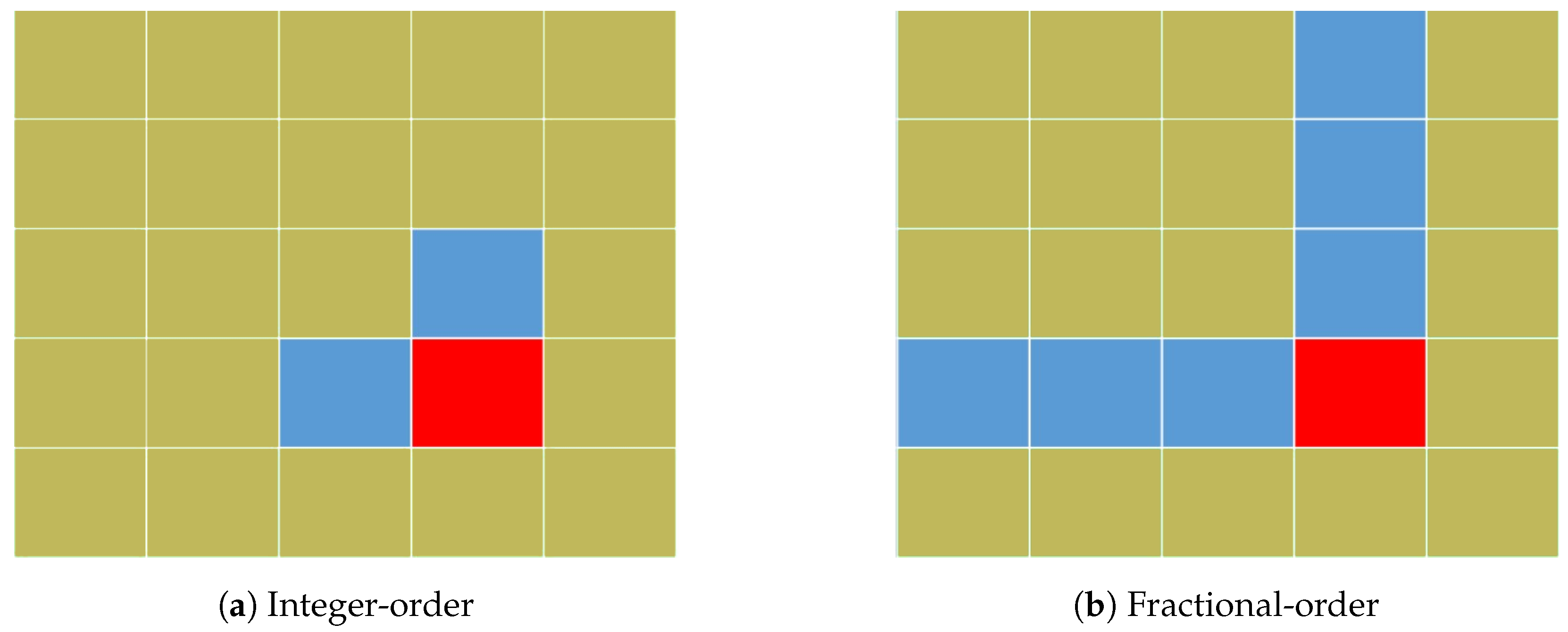
The texture and intricate details within an image often exhibit non-local similarities. However, the domain of first-order gradient variation only encompasses the local attributes of the pixels, thereby rendering the OGS-TV model ineffective in accurately reconstructing the sophisticated texture information within the image. To compensate for these limitations, it is essential to explore a gradient domain that is better suited for retaining the texture information in the image. As illustrated in Figure 1, the FO differential at a given point exhibits non-local properties, meaning that the differential of this point is collectively influenced by the information from multiple surrounding points. Thus, in contrast to the conventional differential form, the FO differential is more congruent with the real-world scenarios when it comes to representing image texture information. Furthermore, the FO differential has a relatively subdued amplification scale for high-frequency information. This attribute is beneficial as it effectively precludes the misidentification of edge information as noise, thereby preventing its removal, and concurrently conserves the edges and contours of the image.
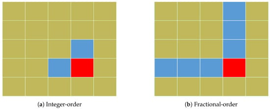
Figure 1.
Distinguishing between integer-order and FO differentials.
In light of the aforementioned analysis, the OGS-FOTVR regularization term has been devised to incorporate the rich texture and complex details inherent in the image, thereby augmenting the quality of the reconstructed image. The structure of the proposed OGS-FOTVR is presented below:
where u and f denote the restored and observed images, respectively. operates as the regularization parameter, while FO differentiation is denoted by . The function is the overlapping group function as defined by Equation (2). The term signifies the data fidelity term, which quantifies the similarity between the restored image u and the observed image f. The component represents the overlapping group sparse FO variational regularization term and serves to characterize the prior information of the restored image. It is crucial to highlight that when , certain low-frequency components escalate non-linearly, while specific high-frequency components diminish non-linearly. Under these circumstances, the frequencies of textures and noises converge, exacerbating the challenge of differentiating between texture and noise. This can lead to the concurrent elimination of texture and noise information. Conversely, when , some low-frequency components decline non-linearly, while certain high-frequency components increase in a non-linear fashion. In this case, the frequency difference between textures and noises is amplified, making it easier to distinguish between them. Although larger values of lead to better preservation of image texture information, they also tend to misclassify some edge and contour information in the image as noise, resulting in blurring and reduced visual quality of the restored image. Therefore, in this paper, we set .
Furthermore, it can be observed that is the overlapping group sparse regularizer defined in the fractional gradient transform domain. Firstly, due to the non-local characteristics of the fractional gradient, the OGS-FOTVR model can effectively suppress the staircase effect and restore more complex texture information in the image. Secondly, by utilizing the overlapping group to measure the sparsity of the fractional gradient variation domain, the model can preserve edge information in the image. Therefore, the OGS-FOTVR model not only mitigates the staircase effect but also achieves a balance between texture and edge restoration.
3.2. Numerical Algorithm
Since the OGS-FOTVR model is a large-scale variational minimization problem, the ADMM algorithm is used to decompose it into several sub-problems for solving. To achieve variable separation, an auxiliary variable v is introduced for variable substitution, transforming the original unconstrained problem (8) into the following constrained problem:
The Equation (10) is characterized as non-convex, primarily due to the inclusion of the function . In this context, signifies a higher-order gradient of the variable u. The function is typically a non-linear operation applied to this gradient, such as an absolute value or a square, which is employed to enhance certain attributes in the solution, such as sparsity or smoothness. The initial term, , is a convex function, as it is a squared Euclidean norm (which is inherently convex) scaled by a positive constant, . However, the overall problem is rendered non-convex due to the incorporation of the non-convex term, . Non-convex optimization problems generally pose a greater challenge than their convex counterparts [33], as they can exhibit multiple local minima, and the solution can become ensnared in these local minima, thereby failing to locate the global minimum. Despite this, numerous practical problems are non-convex, and a variety of strategies have been developed to address them [6,34]. Furthermore, by utilizing the augmented Lagrangian method, the aforementioned constrained problem is converted into an unconstrained problem, specifically constructing an augmented Lagrangian function :
where is the Lagrange multiplier and is the parameter for the quadratic penalty term. Furthermore, the augmented Lagrangian function is obtained using the augmented Lagrangian method, which converts the aforementioned constrained problem into an unconstrained problem. The goal is to find the saddle point of using the alternating direction iterative algorithm, which involves iteratively solving for the minimum values of u and v while maximizing the value of . By initializing the parameters appropriately, the original problem can be transformed into separate coupled sub-problems for solution.
Up to this point, the solution to model (11) is decomposed into a series of sub-problems via ADMM algorithm. Subsequent sections will individually tackle the solutions for these distinct sub-problems.
(1) Sub-problem for u: firstly, the sub-problem for u can be written as follows:
By applying the variational Euler-Lagrange equation, we can determine that the optimal solution u for sub-problem (11) must satisfy the following necessary condition:
where I represents a matrix that is the same size as u, and every element at each position within the matrix is set to 1. It is evident that Equation (12) incorporates a 2D convolution operation, which implies that the optimal solution u cannot be directly extracted from it. This convolution operation is within the spatial domain that can be converted into a direct multiplication operation when this process is executed within the frequency domain. This transformation simplifies the process significantly. Consequently, the numerical solution to the aforementioned equation can be readily obtained by employing the Fourier transform and its corresponding inverse transform as follows:
where and represent the operators for fast Fourier transform (FFT) and fast inverse Fourier transform (IFFT), respectively. In (14), is discrete gradient operator with periodic boundary conditions, and are the x-derivative and y-derivative located at the i-th pixel . present first order difference operator, it can be stated as; . For a comprehensive understanding of image reconstruction, specifically in the context of either integer-order or FO in the Fourier domain, we direct the reader’s attention to references [34,35,36].
To analyze the computational cost of the Equation (14), we can break down the different operations involved and estimate their complexity. The main operations in (14) are the FFT and the IFFT. We also consider the cost of the other arithmetic operations present in (14). At each iteration, the complexity of FFT and IFFT for an n-point transform is , respectively [37,38]. The complexity of applying the gradient operator depends on the specific implementation and the size of the grid points but is usually in the context of fast algorithms. Now, consider the full equation and analyze its complexity as follows:
- Applying :
- Applying the discrete gradient operator and its adjoint: or
- Subtracting :
- Adding :
- Dividing by :
- Adding and :
- Constructing the denominator :
- Applying and for the numerator and denominator:
Since the numerator and denominator each involve FFT and IFFT, the overall complexity for computing is + or . In general, the dominant term in the computational cost will be the FFT and IFFT operations , especially for large values of n. The other operations are typically linear and do not significantly affect the overall complexity when compared to the FFT and IFFT operations.
(2) Sub-problem for v: it is evident that the sub-problem for v is a problem of overlapping group sparse regularization, we have
To facilitate subsequent writing and calculations, it is referred to as:
Due to the complex structural form of this type of problem, the MM algorithm [39] is adopted to solve the above minimization problem. According to the mean value inequality, we have
Based on this, the function at point m can be written as:
According to the inequality (16), it can be proven that and hold. For the convenience of computation, after simplification, can be written in the following form:
where C is a constant that does not depend on v, is a diagonal matrix with its diagonal elements as follows:
where , can be computed using two-dimensional convolution. So far, one alternative function of in Equation (14) can be expressed as follows:
Upon observing the above equation, it is not difficult to notice that the following expressions hold: and . This means that the function satisfies the prerequisite conditions of the MM algorithm. Therefore, in order to minimize according to the MM algorithm, we initialize and then repeatedly minimize the alternative function , i.e.,
where . According to the Euler-Lagrange equation, the numerical solution of sub-problem for v can be obtained as:
(3) Updating Lagrange Multiplier : Finally, according to the ADMM algorithm, the updating form of the Lagrange multiplier is given by:
Therefore, through the aforementioned discussion, the proposed OGS-FOTVR model (8) has been solved using numerical algorithms. The specific solution process is shown in Algorithm 2.
| Algorithm 2 The solution of the proposed OGS-FOTVR is presented in a step-by-step manner |
|
3.3. Convergence Analysis
The convergence of the proposed method, which employs the ADMM, is a crucial aspect to consider. The ADMM algorithm is known for its robustness and efficiency in solving large-scale optimization problems, particularly those involving separable structures, as in our case. The convergence of the ADMM algorithm has been extensively studied and proven in the literature [8,30,40,41]. Moreover, the convergence of the ADMM algorithm in the context of non-convex problems has been studied by Hong et al. [42]. They showed that if the objective function is proper, lower semi-continuous, and the set of optimal solutions is non-empty, then the sequence generated by the ADMM algorithm converges to an optimal solution. In contrast to convex optimization problems where convergence is typically demonstrable, non-convex optimization problems pose a considerably greater challenge due to the necessity of taking various assumptions into account. With regard to the OGS-FOTVR approach, the primary problem is subdivided into several sub-problems, each constituting an optimization problem in its own. These sub-problems are iterative methods, which can be analyzed individually, thus enabling us to provide insights on the convergence characteristics of the OGS-FOTVR. The iterative process involves finding the minimum values of u and v while maximizing the value of , which is the Lagrange multiplier. This process continues until the algorithm converges to a solution that satisfies the constraints of the problem. The convergence of each sub-problem is also guaranteed. For the u sub-problem, the Euler-Lagrange equation is used to find the optimal solution, which is then obtained numerically using the Fourier transform and its inverse [34,36]. For the v sub-problem, the MM algorithm is employed. The MM algorithm is a well-established method for solving optimization problems, and its convergence has been proven under mild conditions [39]. Finally, the Lagrange multiplier is updated according to the ADMM algorithm, which ensures the convergence of the overall method. The updating of continues until the difference between and is sufficiently small, indicating that the solution has converged. The relative error is employed as the stopping criterion. Specifically, the algorithm is designed to stop via this equation, i.e., . Where and indicate the restored images at the current iteration and the previous iteration, respectively. In order to illustrate the convergence analysis, we have graphically represented it in terms of relative error, PSNR and SSIM values in relation to the optimization iterations for OGS-FOTVR, as shown in Figure 2. It is evident that as the number of iterations increases, the relative error demonstrates a decreasing trend and ultimately converges. Moreover, with each iteration of Algorithm 2, there is a noticeable increase in both the PSNR and SSIM values, which eventually reach a point of convergence. This observed pattern provides a clear affirmation of the convergent nature of the proposed OGS-FOTVR, demonstrating its effectiveness and reliability in achieving a stable solution.

Figure 2.
A visual representation of convergence analysis. The analysis employs three test images, namely ‘Pepper’, ‘Boat’, and ‘Cameraman’. These images are processed using a Gaussian kernel of size with a .
In short, the convergence of our proposed method is guaranteed by the properties of the ADMM algorithm and the MM algorithm, as well as the specific structures of the sub-problems. This ensures that our method can effectively and reliably solve the large-scale variational minimization problem posed by the OGS-FOTVR model.
4. Numerical Analysis and Experimental Results
In order to confirm the superior performance and efficacy of the OGS-FOTVR model in image restoration, we carried out a series of numerical experiments. Firstly, the robustness of the OGS-FOTVR model algorithm with respect to initialization is analyzed. Secondly, through numerical experiments, the optimal group size K in the overlapping groups is determined. Finally, a comparative experiment is conducted between the OGS-FOTVR model and other models using test images (as shown in Figure 3) and datasets (SET8, SET12, and SET14) to analyze the advantages of the proposed model. The numerical experiments were conducted on the Lenovo Core i9-12700H, CPU 2.30 GHz, with 32 GB RAM, using the MATLAB R2022a environment. Gaussian white noise with a mean of 0 and variance of is added. The peak signal-to-noise ratio (PSNR) [43] and structural similarity index measure (SSIM) [44] are selected as quantitative evaluation metrics for the numerical experiments. The process for evaluating PSNR (Peak Signal-to-Noise Ratio) and SSIM (Structural Similarity Index Measure) can be articulated using the subsequent equations.
where SPSNR and SSSIM are the values of PSNR and SSIM, respectively, u is the restored image of f, and are the mean and variance of image f, represents the covariance between image f and u, .
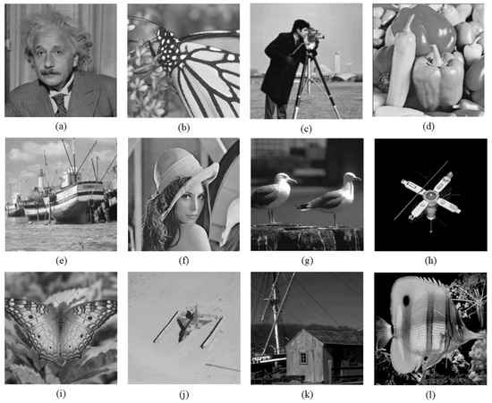
Figure 3.
The test images used for various experiments. (a) Albert Einstein (b) Butterfly1 (c) Cameraman (d) Pepper (e) Boat (f) Lena (g) Seabird (h) satellite (i) Butterfly2 (j) Jet aircraft (k) House (l) Fish.
4.1. Computational Complexity
The computational complexity of the proposed OGS-FOTVR model is primarily determined by the ADMM algorithm, which is used to solve the large-scale variational minimization problem. The ADMM algorithm decomposes the original problem into several sub-problems, each of which can be solved separately, thereby reducing the overall computational complexity. The first sub-problem involves minimizing the augmented Lagrangian function with respect to u. The main computational cost in this step comes from the 2D convolution operation, which is involved in the Euler-Lagrange equation. However, this operation can be efficiently performed in the frequency domain using the FFT, which has a computational complexity of , where n is the number of pixels in the image. The second sub-problem involves minimizing the augmented Lagrangian function with respect to v. This is a problem of OGS regularization, which is solved using the MM algorithm. The MM algorithm involves iterative minimization of an alternative function, which can be efficiently computed using 2D convolution. The computational complexity of this step is also . The third step involves updating the Lagrange multiplier , which can be performed in linear time, i.e., . Therefore, the overall computational complexity of the OGS-FOTVR model is .
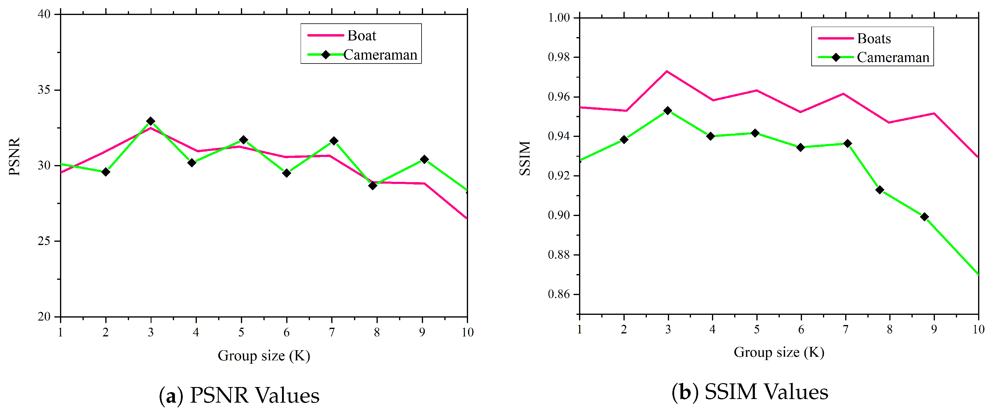
Furthermore, to choose the optimal number of internal iterations N, we selected two images, ‘House’ and ‘Pepper’, from the test images shown in Figure 3. The ‘Pepper’ image is first blurred by a Gaussian kernel and then added with 25% salt-and-pepper noise, while the ‘House’ image is first blurred by a average kernel and then added with 35% salt-and-pepper noise. In this experiment, the group size value in the MM algorithm varies, while the other parameters remain unchanged. However, we already conducted an experiment related to group size K and the visual results in Figure 4 inferred that the optimal group size K is 3. This group size strikes an appropriate balance, providing satisfactory results without overly taxing computational resources. Regarding the MM iteration, a thorough analysis of the data presented in Table 1 points to a suitable value of 5. This value notably succeeds in managing the trade-off between the PSNR and SSIM parameters and the requisite CPU time for executing the algorithm. Therefore, it can be concluded that employing a group size of 3 and an MM iteration of 5, leads to an efficient balancing of performance.

Figure 4.
Comparison of average PSNR and SSIM values for different cluster sizes K.

Table 1.
Running time with varied quantities of inner iterations (N).
4.2. Ablation Study
This section is dedicated to a thorough exploration via an ablation study. The primary objective of this research endeavor is to conduct a precise evaluation of each component within our proposed model, considering their individual contributions to the overall model’s performance. The “Lena” image and corresponding parameters were chosen for this study to ensure uniformity with the other experimental analyses conducted throughout the paper. The image is corrupted by adding 30% noise. During the initial stages of our experiment, we utilized the OGS-TV technique to facilitate image restoration. We observed that OGS-TV achieved a PSNR value of , signifying a high-speed performance. Subsequently, our investigative efforts were directed towards the evaluation of the second module, i.e., FOTVR. The outcomes derived from FOTVR indicated a marginal increase in PSNR value and CPU time compared to those obtained from the OGS-TV method. As our experimental procedure progressed, we merged both modules to validate the net effect of our proposed methodology. The results of the combined modules implemented in this study achieved enhanced image restoration results, underpinned by superior PSNR values. The findings in Table 2 signify that an integrative approach tends to substantially improve the overall quality of the restored image. Note that the total number of iterations is set to 150, the group size K is set to 3, and the remaining parameters for the ablation study are kept the same as those used in our other experiments.

Table 2.
Ablation study of the proposed model.
4.3. Robustness of the Model to the Initial Value
To verify the robustness of the model to the initial value , different levels of Gaussian noise are added to the test images, resulting in degraded images at various noise levels. Four different initial values are selected, i.e., , , , and f, where the Matlab built-in functions zeros and ones generate pixel matrices with all elements being 0 and 1, respectively, while random represents randomly generated pixel matrices with values between 0 and 1 following a Gaussian distribution. Subsequently, the OGS-FOTVR model underwent a rigorous evaluation process under varied initialization conditions. For each initial setting, average PSNR and SSIM values of the rejuvenated images are meticulously calculated and listed in Table 3. A discerning analysis of the data presented in Table 3 reveals that alterations in initial values wield a rather insubstantial influence on image recovery performance when the noise level remains constant. However, as the noise level escalates, the sway of initial values on the model’s outcomes starts to incrementally intensify. This escalation, though perceptible, can be categorized as negligible in its tangible impact. Consequently, the OGS-FOTVR model can be lauded for its commendable robustness in the face of varying initialization parameters, reinforcing its versatility and steadfastness as an exemplary tool in image restoration.

Table 3.
Examining the robustness of PSNR and SSIM with respect to initial values of .
4.4. Group Size (K)
In order to determine the ideal group size of K, we conducted a denoising experiment subjected to a salt-and-pepper noise with . We conducted this investigation by holding all other factors constant and changing only the value of K. We tested different K values, ranging from 1 to 8, i.e., (K = 1, 2, 3, …, 8), and applied these to a series of experiments. In these experiments, we attempted to reduce the noise in test images, i.e., Boat and Cameraman. To measure the effectiveness of our approach, we calculated the average values in terms of PSNR and SSIM. We plotted these results in Figure 4, showing the connection between the group size K and the image quality. Figure 4 illustrates that when K = 3, the proposed method attained better scores. We also discovered that the value of K acts similarly to a scaling factor in the noise reduction process. If K is too big or too small, it can affect the visual appearance of the final image. However, based on the given findings, we chose K = 3 in our all experiments.
4.5. Impact of Parameters and
To assess the impact of parameters and on experimental outcomes, this research utilized two test images, namely “Boat” and “Pepper”. These images are subjected to varying values of and under different noise levels. The results in Table 4 highlight the corresponding and values that yielded the highest PSNR for the restored images at different noise levels. Examining the data in Table 4, it is evident that as the noise level increases from = 10 to = 20, opting for a smaller fidelity term coefficient becomes necessary. This decision amplifies the influence of the regularization term on the model, thereby achieving optimal denoising outcomes.

Table 4.
Quantifying the impact of and on denoising outcomes.
4.6. Impact of Parameter
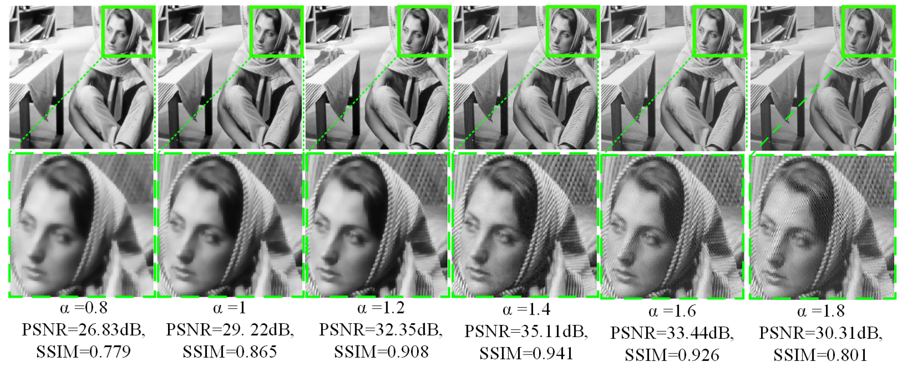
The FO differentiation degree has a significant impact on both denoising and texture preservation. An experiment is carried out to evaluate the impact of the FO parameter on the performance of the proposed model. For this experiment, the ‘Barbara’ image is taken from the SET14 dataset and various FO values of are selected for its effect on image reconstruction. During this evaluation, the parameter is set to . Figure 5 presents the reconstructed results and their respective magnified sections, each corresponding to a different FO , PSNR and SSIM. It is evident that when the FO 1, the images reconstructed by OGS-FOTVR tend to lose more textures and details. When , the results obtained by the OGS-FOTVR are equivalent to those of the TV model [10]. As exceeds 1, the retention of texture details in the image enhances. Nevertheless, as the value of nears 2, the amplification of texture frequency is increased, resulting in a form of visual disturbance or noise. Therefore, to strike an optimal balance, we have set to in our experiments.
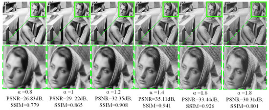
Figure 5.
Exploring the effect of FO parameter .
4.7. Comparison of Numerical Experimental Results
In order to substantiate the effectiveness and superior performance of the proposed model, we have elected to conduct a comparative analysis with several established models. These include the TGV [45], TFOTV [46], FOTV [47], CHONTV [48], L0_OGS [49], NMG [50], and HPWH_OGS [51]. Each of these models represents a distinct approach to image processing, thereby providing a comprehensive spectrum for comparison. This comparative analysis not only underscores the strengths of our proposed model but also highlights areas for potential improvement and future exploration. By examining the performance of our model against these established methods, we aim to demonstrate its unique capabilities and potential applications in the field of image processing.
4.7.1. Comparative Experimental Results for Different Noise Levels
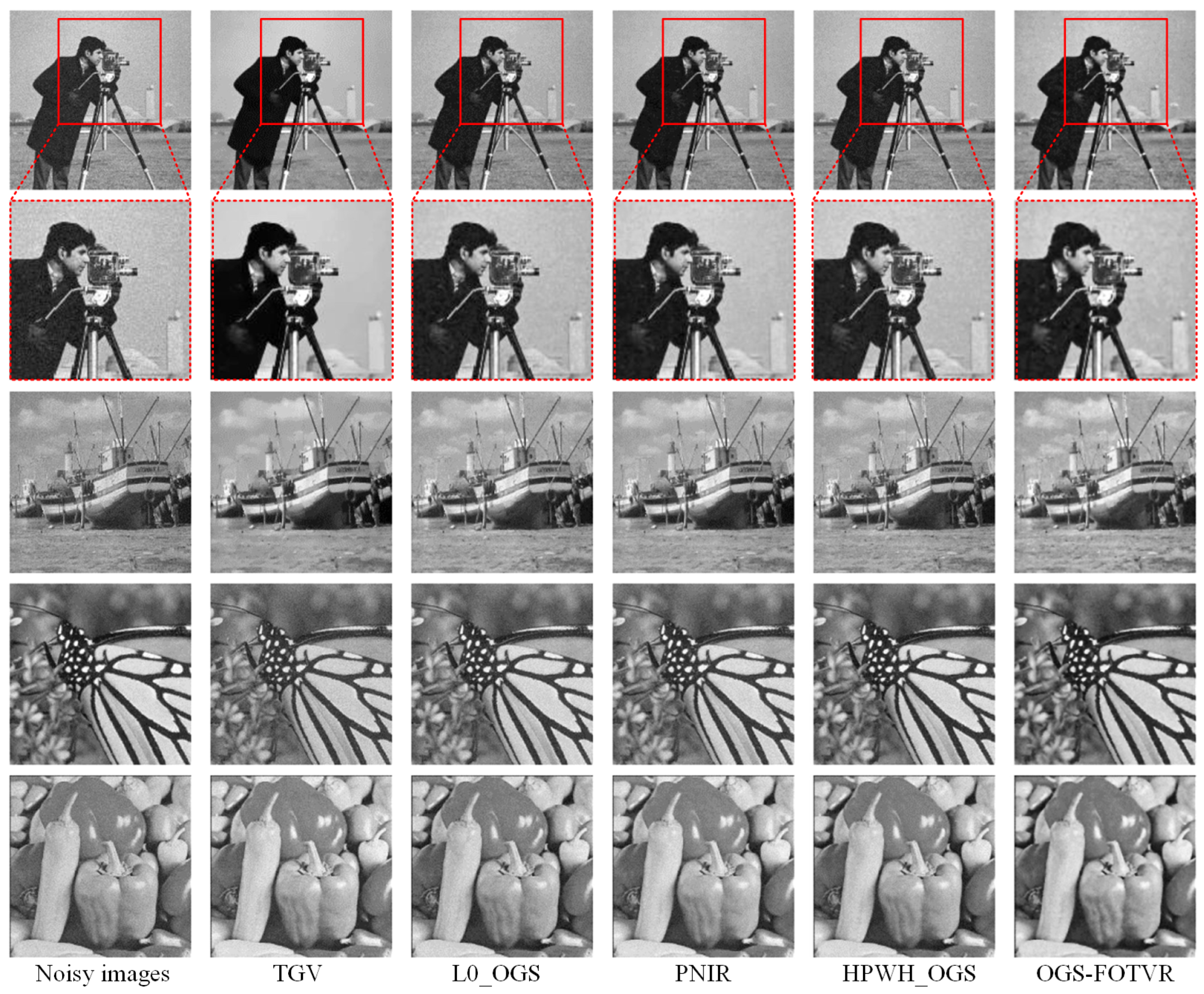
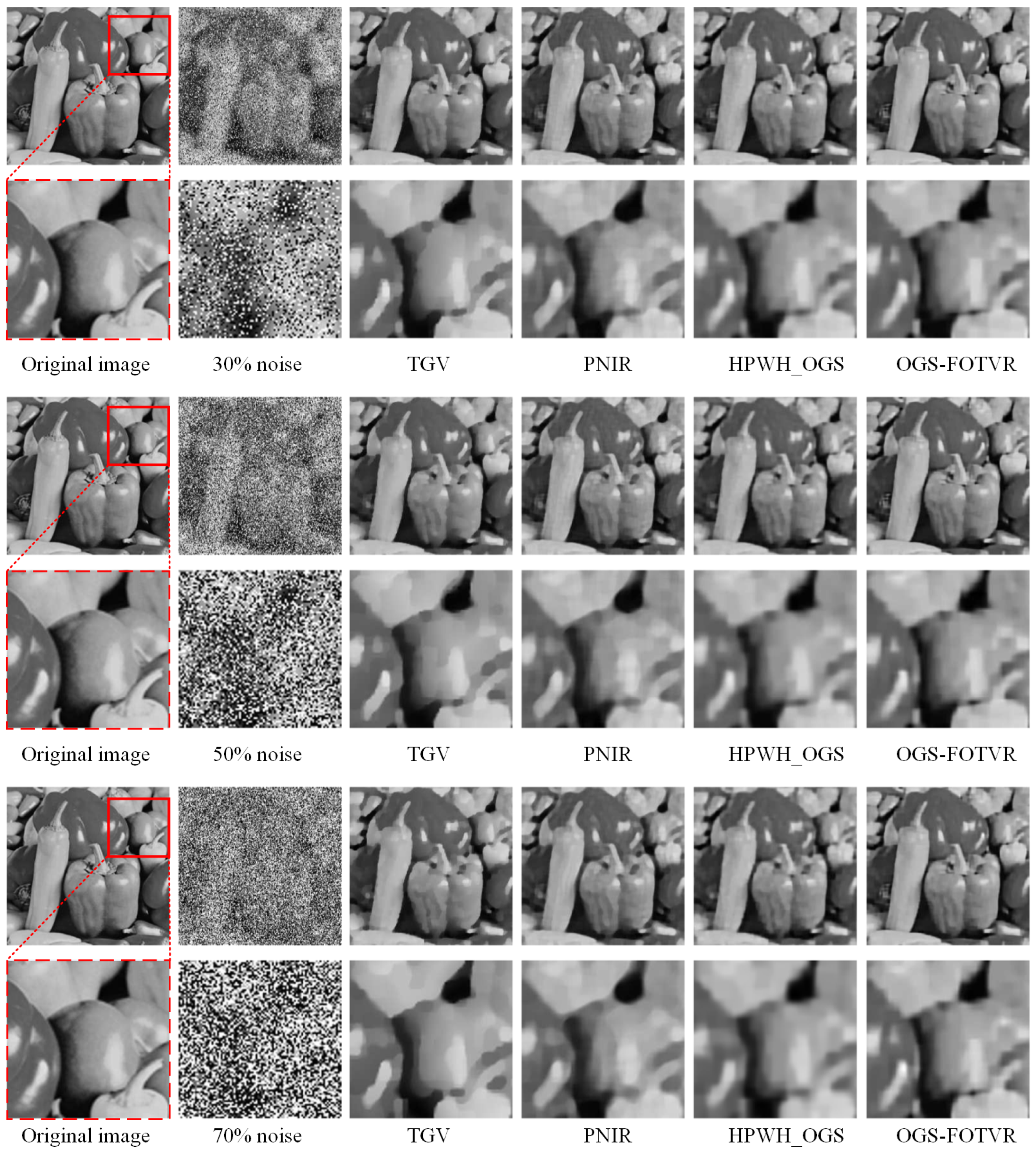
This section presents a comparative analysis of the denoising capabilities of our proposed model alongside an array of established models under noise levels of = 10 in Figure 6 and 30%, 50%, 70% in Figure 7, respectively.
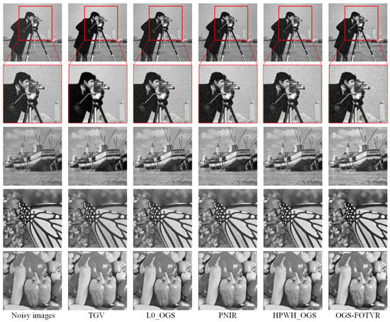
Figure 6.
Exploring denoising capabilities of various models at = 10.
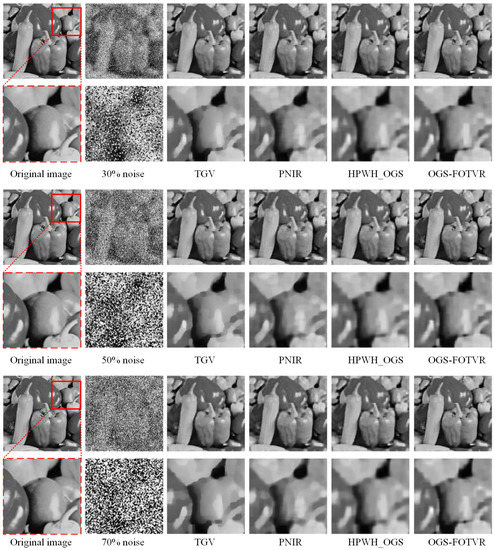
Figure 7.
The visual outcomes of pepper image, wherein a Gaussian blur kernel of size 15 × 15 with a standard deviation of 5 has been applied, in conjunction with salt-and-pepper noise at varying intensities of 30%, 50%, and 70%.
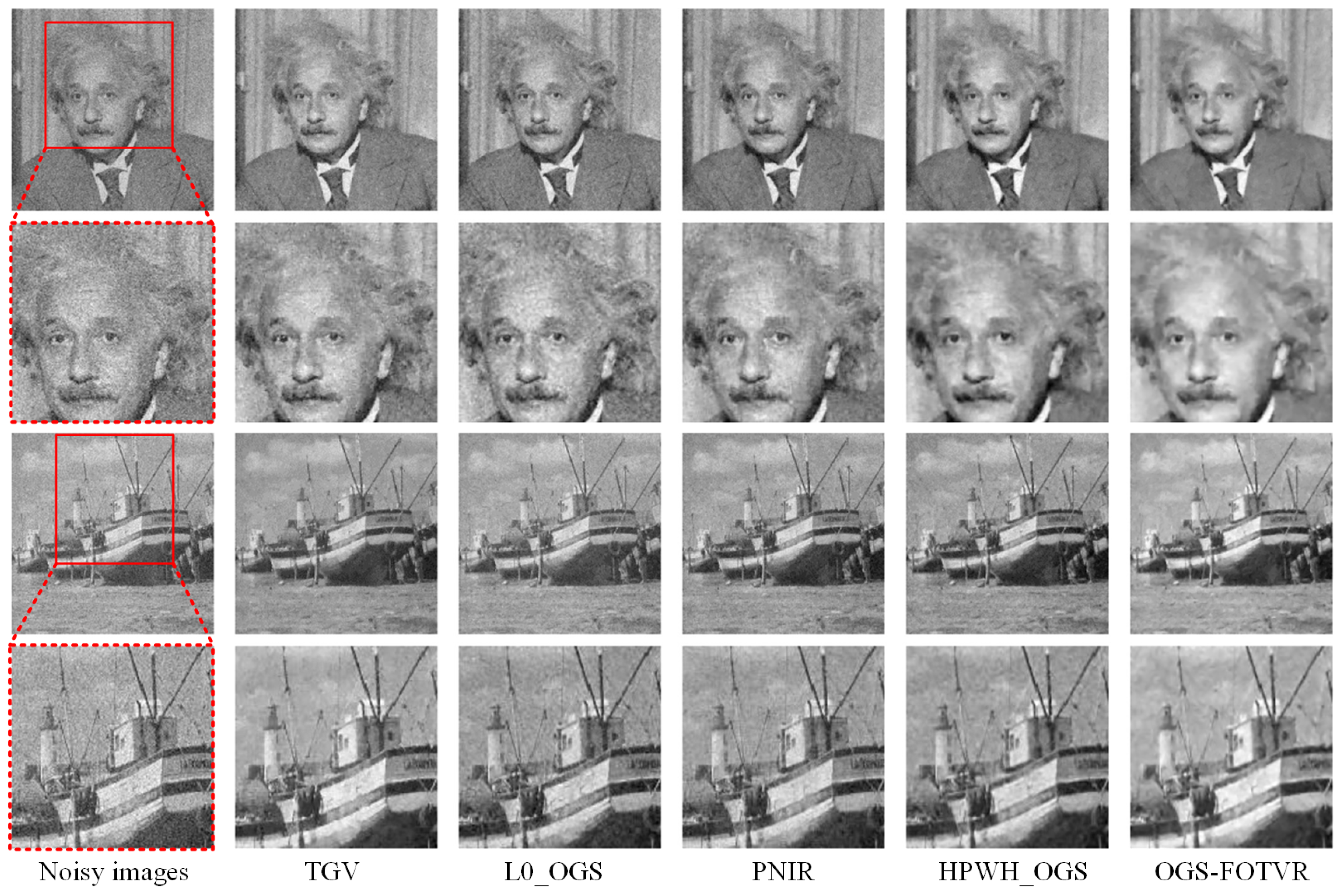
The results serve as visual aids in highlighting the performance of these models. It is evident from the given visual comparison that the TVG [45] model excels in preserving the edges within images, albeit at the cost of generating stark staircase artifacts in regions of smoothness. For instance, the “cameraman” image in Figure 6 shows that when applying the TGV [45] model, the sky background reveals distinct segments of constant regions. This indicates a failure to adeptly capture the intricate oscillations and textures within these areas. In contrast, the L0_OGS [49], PNIR [52], and HPWH_OGS [51] models demonstrate a more proficient depiction of the texture and fine details, while simultaneously mitigating the staircasing effect. Among these, the PNIR [52] model employs non-local gradient information of pixels, which aligns the restoration more closely with the true nature of the image. On the other hand, the OGS-FOTVR model takes into account the interrelation among pixel blocks within the image. This approach to measuring the sparsity of image gradients resonates more accurately with the inherent attributes of natural images, thus resulting in commendable restoration outcomes.
Furthermore, the TGV [45] and L0_OGS [49] models are not ideal for recovering complex texture areas, such as the rich texture part of the “pepper” image in Figure 7. It is easy to see that these two models’ recovery effects on the texture preservation are just average. Compared to the other two models, the HPWH_OGS [51] not only alleviates the step effect but also effectively recovers the complex detail areas in the image. However, this model contains a large number of parameters to be determined, making it difficult to ensure the optimality of the chosen parameters during image recovery. However, the OGS-FOTVR model not only overcomes these shortcomings, but also contains the fewest parameters to be determined; moreover, it can suppress the generation of constant segment regions during image recovery, while also better recovering complex textures or detail areas. Figure 8 illustrates the restoration results of the models at = 20. It can be observed that, except for the TV model, other models exhibit minimal staircase artifacts. Additionally, when examining the boat structure in the ‘Boat’ image and the forehead area in the ‘Albert Einstein’ image, it becomes apparent that the OGS-FOTVR model captures more information in texture and detail regions. Therefore, compared to other models, the OGS-FOTVR model excels in preserving edge contours and restoring complex texture details. Moreover, Table 5 presents the numerical experimental results for image restoration at different noise levels. From Table 5, it can be seen that the OGS-FOTVR model has better PSNR and SSIM values compared to other models, further confirming its superiority. However, it is important to note that OGS-FOTVR relies on OGS and FOTVR. Therefore, it uses more computer processing time compared to FOTV [47]. Periodically, this could require additional iterations, representing a potential disadvantage in the context of resource utilization and efficiency. However, this shortcoming is partially offset by the remarkable performance demonstrated by the model in terms of restoration outcomes. Consequently, the cumulative benefits in relation to image quality could feasibly counterbalance the increased computational cost.
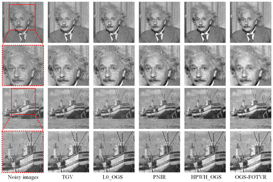
Figure 8.
Comparing denoising results of prior and our models at = 20.

Table 5.
Quantitative analysis of prior and our denoising models in terms of PSNR, SSIM and CPU time.
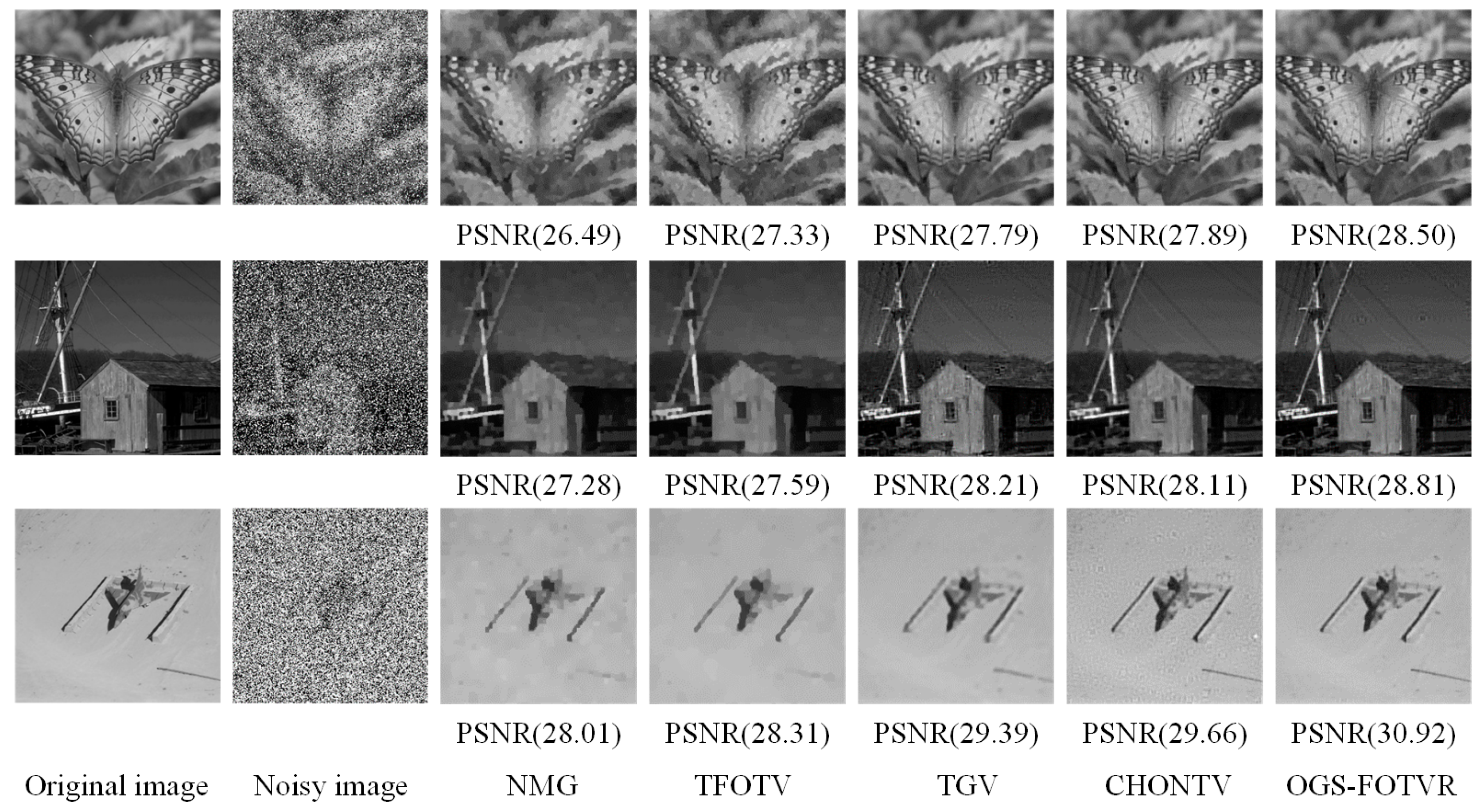
In order to gain a more thorough understanding of the examination outcomes, we have visualized some reconstructed images. Figure 9 showcases the results of image reconstruction for a variety of models applied to butterfly, boat, house, and airplane images, which have been blurred at impulse noise intensities ranging from 25% to 50%. It is apparent from the visual results that the model proposed in this study demonstrates superior image reconstruction performance across all noise levels, exhibiting PSNR values that surpass other leading models including NMG [50], TFOTV [46], TVG [45], CHONTV [48]. The model introduced in this paper exhibits robust efficacy in image reconstruction, irrespective of the noise levels. It is noteworthy that, despite being subjected to significant noise interference, our suggested algorithm consistently produces reconstructed images with outstanding visual clarity.
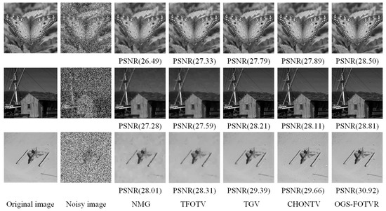
Figure 9.
Comparing denoising results of prior and our models at = 20.
4.7.2. Comparison of Test Results on Different Datasets
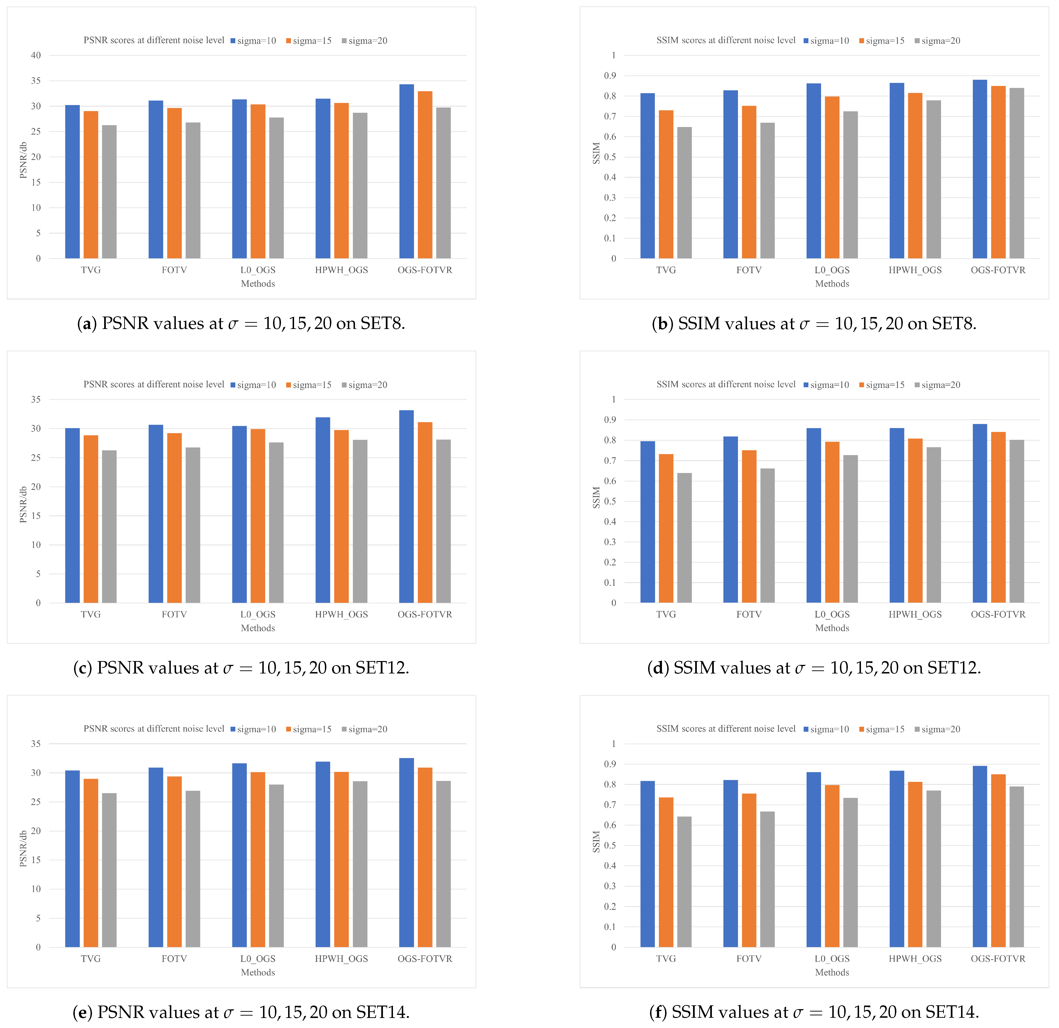
In pursuit of rigorously appraising the capabilities of the OGS-FOTVR model, an incisive analysis is undertaken employing three bespoke datasets, constructed from an amalgamation of synthetic and natural images in varying states of degradation [53]. These datasets, herein referred to as SET8, SET12, and SET14, comprise 20, 25, and 15 images, respectively. A compendium of numerical experiments is meticulously executed to facilitate a comparative analysis of the denoising performance of the OGS-FOTVR model with other prior models, including TVG [45], FOTV [47], L0_OGS [49], and HPWH_OGS [51], over a range of noise levels. The evaluative paradigm is anchored in the utilization of PSNR and SSIM as the cardinal metrics, which offer invaluable insights into the fidelity and structural integrity of the denoised images. Figure 10 elucidates the average PSNR and SSIM values for the images post-restoration, aggregated from the aforementioned datasets. A detailed analysis of Figure 10 clearly illustrates that the OGS-FOTVR model offers not just promising but also evidently superior denoising capabilities when compared to other variational models across a comprehensive range of datasets. This superiority, in terms of both quantitative metrics and likely perceptual quality, underscores the potency of the OGS-FOTVR model as a quintessential tool for image restoration. Furthermore, this efficacy paves the way for extensive applications in various domains that necessitate high-quality image reconstruction, such as medical imaging, satellite imagery, and digital forensics. The OGS-FOTVR model’s adaptability and performance make it a compelling choice for researchers and practitioners seeking state-of-the-art denoising methodologies. This work heralds a noteworthy advancement in image processing and restoration techniques, engendering new possibilities for further research and development.
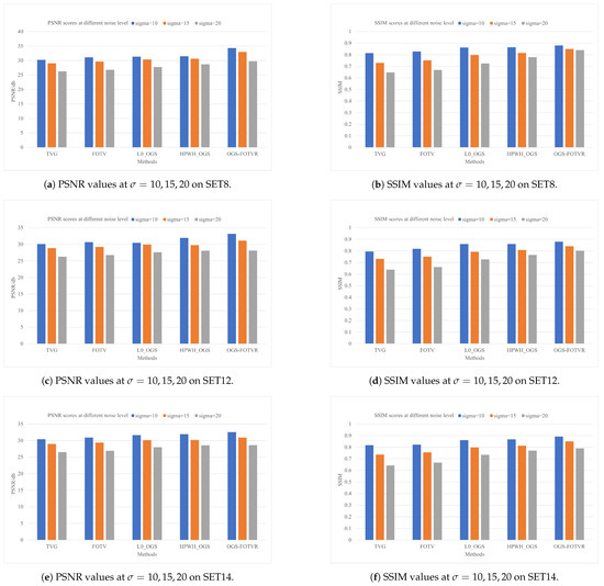
Figure 10.
Performance analysis of average PSNR and SSIM result for denoising mdoels on SET8, SET12, and SET14.
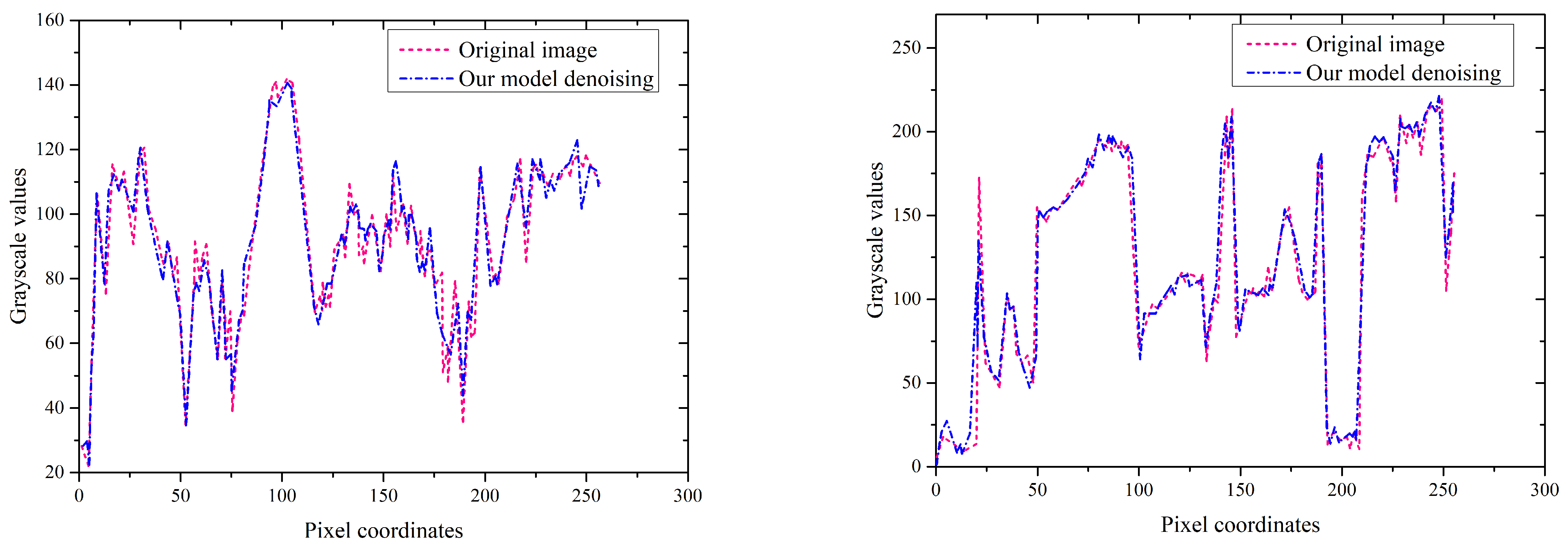
Furthermore, natural images often exhibit textures or details characterized by oscillatory patterns. This concept is exemplified in Figure 11, which provides a comparative analysis between the local cross-sections of the original images, “Cameraman” and “Pepper”, and their respective restored versions. In this context, the x-axis denotes the position of pixel points within the image cross-section, while the y-axis corresponds to the gray value of each pixel point. Upon examination of Figure 11, it becomes evident that both images encompass numerous oscillatory regions, signifying their rich texture and intricate detail content. When the OGS-FOTVR model is employed for restoration, the resulting images in the oscillatory regions bear a close resemblance to the original images. This successful approximation illustrates the commendable efficacy of the OGS-FOTVR model in processing images replete with complex textures and detailed information.
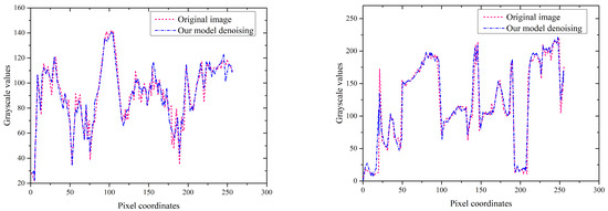
Figure 11.
The local cross-section u(100,:) of the denoised image and the corresponding real image at = 10.
5. Conclusions
In response to the complexities associated with noisy images that contain intricate textures or elaborate details, we have developed the OGS-FOTVR model. This innovative approach leverages the concept of overlapping groups to encapsulate the sparsity within the FO variation domain. The result is a model that not only mitigates staircase artifacts but also meticulously preserves image edges, while effectively recovering complex textures and nuanced features. A powerful algorithmic framework ADMM is employed to efficiently solve the model using the MM algorithm. The experimental results reveal that the OGS-FOTVR model performs better than traditional variational models, demonstrating its robustness during initialization and its outstanding performance features. However, it is important to note that the OGS-FOTVR model does require manual parameter tuning, particularly to determine the FO difference order within the model. This requirement introduces an additional layer of complexity to the experimental process, increasing the overhead associated with implementing the model. Despite this, the benefits offered by the OGS-FOTVR model in terms of image denoising performance make it a promising approach for handling images with complex textures and details. Consequently, a salient avenue for future research lies in the realization of adaptive determination of the FO difference order in the model, tailored to distinct images. This would contribute toward streamlining the model’s implementation and augmenting its practical utility in image denoising applications.
Author Contributions
Conceptualization and Methodology, J.A.B. and A.K.; Software, J.A.B. and Z.R.; Investigation, Z.R.; Data curation, Z.R.; Writing—original draft, J.A.B. Funding acquisition, A.K. All authors have read and agreed to the published version of the manuscript.
Funding
This research was sponsored by the Guangzhou Government Project under Grant No. 62216235 and the National Natural Science Foundation of China (Grant No. 622260-1).
Data Availability Statement
The datasets and code will be made available upon request, through the First and Corresponding authors.
Conflicts of Interest
The authors declare no conflict of interest.
References
- Kongskov, R.D.; Dong, Y.; Knudsen, K. Directional total generalized variation regularization. BIT Numer. Math. 2019, 59, 903–928. [Google Scholar] [CrossRef]
- Li, H.; Duan, X.L. SAR Ship Image Speckle Noise Suppression Algorithm Based on Adaptive Bilateral Filter. Wirel. Commun. Mob. Comput. 2022, 2022, 9392648. [Google Scholar] [CrossRef]
- Bai, J.; Feng, X.C. Fractional-order anisotropic diffusion for image denoising. IEEE Trans. Image Process. 2007, 16, 2492–2502. [Google Scholar] [CrossRef]
- Kumar, S.; Alam, K.; Chauhan, A. Fractional derivative based nonlinear diffusion model for image denoising. SeMA J. 2022, 79, 355–364. [Google Scholar] [CrossRef]
- Yang, J.H.; Zhao, X.L.; Ma, T.H.; Chen, Y.; Huang, T.Z.; Ding, M. Remote sensing images destriping using unidirectional hybrid total variation and nonconvex low-rank regularization. J. Comput. Appl. Math. 2020, 363, 124–144. [Google Scholar] [CrossRef]
- Adam, T.; Paramesran, R. Image denoising using combined higher order non-convex total variation with overlapping group sparsity. Multidimens. Syst. Signal Process. 2019, 30, 503–527. [Google Scholar] [CrossRef]
- Xi, Y.; Qiao, Z.; Wang, W.; Niu, L. Study of CT image reconstruction algorithm based on high order total variation. Optik 2020, 204, 163814. [Google Scholar] [CrossRef]
- Wu, T.; Gu, X.; Wang, Y.; Zeng, T. Adaptive total variation based image segmentation with semi-proximal alternating minimization. Signal Process. 2021, 183, 108017. [Google Scholar] [CrossRef]
- Zhang, Y.; Niu, G.; Sugiyama, M. Learning noise transition matrix from only noisy labels via total variation regularization. In Proceedings of the International Conference on Machine Learning, PMLR, Virtual, 18–24 July 2021; pp. 12501–12512. [Google Scholar]
- Phan, T.D.K. A weighted total variation based image denoising model using mean curvature. Optik 2020, 217, 164940. [Google Scholar] [CrossRef]
- Zheng, Y.; Jeon, B.; Zhang, J.; Chen, Y. Adaptively determining regularisation parameters in non-local total variation regularisation for image denoising. Electron. Lett. 2015, 51, 144–145. [Google Scholar] [CrossRef]
- Jidesh, P.; Febin, I. Estimation of noise using non-local regularization frameworks for image denoising and analysis. Arab. J. Sci. Eng. 2019, 44, 3425–3437. [Google Scholar] [CrossRef]
- Gong, B.; Schullcke, B.; Krueger-Ziolek, S.; Zhang, F.; Mueller-Lisse, U.; Moeller, K. Higher order total variation regularization for EIT reconstruction. Med. Biol. Eng. Comput. 2018, 56, 1367–1378. [Google Scholar] [CrossRef] [PubMed]
- Zhao, M.; Wang, Q.; Muniru, A.N.; Ning, J.; Li, P.; Li, B. Numerical Calculation of Partial Differential Equation Deduction in Adaptive Total Variation Image Denoising. In Proceedings of the 2019 12th International Congress on Image and Signal Processing, BioMedical Engineering and Informatics (CISP-BMEI), Suzhou, China, 19–21 October 2021; IEEE: New York, NY, USA, 2019; pp. 1–6. [Google Scholar]
- Ding, M.; Huang, T.Z.; Wang, S.; Mei, J.J.; Zhao, X.L. Total variation with overlapping group sparsity for deblurring images under Cauchy noise. Appl. Math. Comput. 2019, 341, 128–147. [Google Scholar] [CrossRef]
- Wang, L.; Chen, Y.; Lin, F.; Chen, Y.; Yu, F.; Cai, Z. Impulse noise denoising using total variation with overlapping group sparsity and Lp-pseudo-norm shrinkage. Appl. Sci. 2018, 8, 2317. [Google Scholar] [CrossRef]
- Deng, S.W.; Han, J.Q. Adaptive overlapping-group sparse denoising for heart sound signals. Biomed. Signal Process. Control 2018, 40, 49–57. [Google Scholar] [CrossRef]
- Yang, Q.; Chen, D.; Zhao, T.; Chen, Y. Fractional calculus in image processing: A review. Fract. Calc. Appl. Anal. 2016, 19, 1222–1249. [Google Scholar] [CrossRef]
- Wang, Y.; He, Y.; Zhu, Z. Study on fast speed fractional order gradient descent method and its application in neural networks. Neurocomputing 2022, 489, 366–376. [Google Scholar] [CrossRef]
- He, N.; Wang, J.B.; Zhang, L.L.; Lu, K. An improved fractional-order differentiation model for image denoising. Signal Process. 2015, 112, 180–188. [Google Scholar] [CrossRef]
- Smith, D.; Gopinath, S.; Arockiaraj, F.G.; Reddy, A.N.K.; Balasubramani, V.; Kumar, R.; Dubey, N.; Ng, S.H.; Katkus, T.; Selva, S.J.; et al. Nonlinear Reconstruction of Images from Patterns Generated by Deterministic or Random Optical Masks—Concepts and Review of Research. J. Imaging 2022, 8, 174. [Google Scholar] [CrossRef]
- Appati, J.K.; Owusu, E.; Agbo Tettey Soli, M.; Adu-Manu, K.S. A novel convolutional Atangana-Baleanu fractional derivative mask for medical image edge analysis. J. Exp. Theor. Artif. Intell. 2022, 1–23. [Google Scholar] [CrossRef]
- Al-Shamasneh, A.R.; Ibrahim, R.W. Image Denoising Based on Quantum Calculus of Local Fractional Entropy. Symmetry 2023, 15, 396. [Google Scholar] [CrossRef]
- Wang, W.; Li, F.; Ng, M.K. Structural similarity-based nonlocal variational models for image restoration. IEEE Trans. Image Process. 2019, 28, 4260–4272. [Google Scholar] [CrossRef] [PubMed]
- Li, M.M.; Li, B.Z. A novel weighted anisotropic total variational model for image applications. Signal Image Video Process. 2022, 16, 211–218. [Google Scholar] [CrossRef]
- Zhang, T.; Peng, Z.; Wu, H.; He, Y.; Li, C.; Yang, C. Infrared small target detection via self-regularized weighted sparse model. Neurocomputing 2021, 420, 124–148. [Google Scholar] [CrossRef]
- Yao, W.; Guo, Z.; Sun, J.; Wu, B.; Gao, H. Multiplicative noise removal for texture images based on adaptive anisotropic fractional diffusion equations. SIAM J. Imaging Sci. 2019, 12, 839–873. [Google Scholar] [CrossRef]
- You, J.; Jiao, Y.; Lu, X.; Zeng, T. A nonconvex model with minimax concave penalty for image restoration. J. Sci. Comput. 2019, 78, 1063–1086. [Google Scholar] [CrossRef]
- Sahin, M.F.; Alacaoglu, A.; Latorre, F.; Cevher, V. An inexact augmented Lagrangian framework for nonconvex optimization with nonlinear constraints. Adv. Neural Inf. Process. Syst. 2019, 32. [Google Scholar] [CrossRef]
- Jiang, L.; Huang, J.; Lv, X.G.; Liu, J. Alternating direction method for the high-order total variation-based Poisson noise removal problem. Numer. Algorithms 2015, 69, 495–516. [Google Scholar] [CrossRef]
- Liu, J.; Huang, T.Z.; Selesnick, I.W.; Lv, X.G.; Chen, P.Y. Image restoration using total variation with overlapping group sparsity. Inf. Sci. 2015, 295, 232–246. [Google Scholar] [CrossRef]
- Liu, Q.; Sun, L.; Gao, S. Non-convex fractional-order derivative for single image blind restoration. Appl. Math. Model. 2022, 102, 207–227. [Google Scholar] [CrossRef]
- Liu, Q.; Liu, J.; Xiong, B.; Liang, D. A non-convex gradient fidelity-based variational model for image contrast enhancement. EURASIP J. Adv. Signal Process. 2014, 2014, 1–9. [Google Scholar] [CrossRef]
- Wali, S.; Li, C.; Imran, M.; Shakoor, A.; Basit, A. Level-set evolution for medical image segmentation with alternating direction method of multipliers. Signal Process. 2023, 211, 109105. [Google Scholar] [CrossRef]
- Helou, M.E.; Dümbgen, F.; Achanta, R.; Süsstrunk, S. Fourier-domain optimization for image processing. arXiv 2018, arXiv:1809.04187. [Google Scholar]
- Wali, S.; Li, C.; Basit, A.; Shakoor, A.; Memon, R.A.; Rahim, S.; Samina, S. Fast and adaptive boosting techniques for variational based image restoration. IEEE Access 2019, 7, 181491–181504. [Google Scholar] [CrossRef]
- Tao, M.; Yang, J.; He, B. Alternating Direction Algorithms for Total Variation Deconvolution in Image Reconstruction; TR0918; Department of Mathematics, Nanjing University: Nanjing, China, 2009. [Google Scholar]
- Figueiredo, M.A.; Bioucas-Dias, J.M.; Nowak, R.D. Majorization–minimization algorithms for wavelet-based image restoration. IEEE Trans. Image Process. 2007, 16, 2980–2991. [Google Scholar] [CrossRef]
- Zhao, Y.; Wu, C.; Dong, Q.; Zhao, Y. An accelerated majorization-minimization algorithm with convergence guarantee for non-Lipschitz wavelet synthesis model. Inverse Probl. 2021, 38, 015001. [Google Scholar] [CrossRef]
- Boyd, S.; Parikh, N.; Chu, E.; Peleato, B.; Eckstein, J. Distributed optimization and statistical learning via the alternating direction method of multipliers. Found. Trends Mach. Learn. 2011, 3, 1–122. [Google Scholar] [CrossRef]
- Li, D.; Jiang, T.; Jin, Q.; Zhang, B. Adaptive Fractional Order Total Variation Image Denoising via the Alternating Direction Method of Multipliers. In Proceedings of the 2020 Chinese Control And Decision Conference (CCDC), Hefei, China, 22–24 August 2020; IEEE: New York, NY, USA, 2020; pp. 3876–3881. [Google Scholar]
- Hong, M.; Luo, Z.Q.; Razaviyayn, M. Convergence analysis of alternating direction method of multipliers for a family of nonconvex problems. SIAM J. Optim. 2016, 26, 337–364. [Google Scholar] [CrossRef]
- Mozhaeva, A.; Streeter, L.; Vlasuyk, I.; Potashnikov, A. Full reference video quality assessment metric on base human visual system consistent with PSNR. In Proceedings of the 2021 28th Conference of Open Innovations Association (FRUCT), Moscow, Russia, 27–29 January 2021; IEEE: New York, NY, USA, 2021; pp. 309–315. [Google Scholar]
- Bakurov, I.; Buzzelli, M.; Schettini, R.; Castelli, M.; Vanneschi, L. Structural similarity index (SSIM) revisited: A data-driven approach. Expert Syst. Appl. 2022, 189, 116087. [Google Scholar] [CrossRef]
- Wali, S.; Zhang, H.; Chang, H.; Wu, C. A new adaptive boosting total generalized variation (TGV) technique for image denoising and inpainting. J. Vis. Commun. Image Represent. 2019, 59, 39–51. [Google Scholar] [CrossRef]
- Zhu, J.; Wei, J.; Lv, H.; Hao, B. Truncated Fractional-Order Total Variation for Image Denoising under Cauchy Noise. Axioms 2022, 11, 101. [Google Scholar] [CrossRef]
- Zhu, J.; Wei, J.; Hao, B. Fast algorithm for box-constrained fractional-order total variation image restoration with impulse noise. IET Image Process. 2022, 16, 3359–3373. [Google Scholar] [CrossRef]
- Adam, T.; Paramesran, R.; Mingming, Y.; Ratnavelu, K. Combined higher order non-convex total variation with overlapping group sparsity for impulse noise removal. Multimed. Tools Appl. 2021, 80, 18503–18530. [Google Scholar] [CrossRef]
- Yin, M.; Adam, T.; Paramesran, R.; Hassan, M.F. An L0-overlapping group sparse total variation for impulse noise image restoration. Signal Process. Image Commun. 2022, 102, 116620. [Google Scholar] [CrossRef]
- He, W.; Yao, Q.; Li, C.; Yokoya, N.; Zhao, Q.; Zhang, H.; Zhang, L. Non-local meets global: An iterative paradigm for hyperspectral image restoration. IEEE Trans. Pattern Anal. Mach. Intell. 2020, 44, 2089–2107. [Google Scholar] [CrossRef] [PubMed]
- He, Y.; Zhu, J.; Hao, B. Hybrid priors based on weighted hyper-Laplacian with overlapping group sparsity for poisson noise removal. Signal Image Video Process. 2023, 17, 2607–2615. [Google Scholar] [CrossRef]
- Jon, K.; Liu, J.; Lv, X.; Zhu, W. Poisson noisy image restoration via overlapping group sparse and nonconvex second-order total variation priors. PLoS ONE 2021, 16, e0250260. [Google Scholar]
- Sun, L.; Hays, J. Super-resolution from internet-scale scene matching. In Proceedings of the 2012 IEEE International conference on computational photography (ICCP), Seattle, WA, USA, 28–29 April 2012; IEEE: New York, NY, USA, 2012; pp. 1–12. [Google Scholar]
Disclaimer/Publisher’s Note: The statements, opinions and data contained in all publications are solely those of the individual author(s) and contributor(s) and not of MDPI and/or the editor(s). MDPI and/or the editor(s) disclaim responsibility for any injury to people or property resulting from any ideas, methods, instructions or products referred to in the content. |
© 2023 by the authors. Licensee MDPI, Basel, Switzerland. This article is an open access article distributed under the terms and conditions of the Creative Commons Attribution (CC BY) license (https://creativecommons.org/licenses/by/4.0/).

