Abstract
This paper proposes a wireless channel equalization method applied to the constant modulus blind equalization system, which addresses the slow convergence and strong randomness in the initialization of equalizer weights in the constant modulus blind equalization algorithm (CMA) by introducing a hybrid arithmetic whale optimization algorithm (HAWOA). The mean square error in the CMA is utilized as the cost function for the HAWOA to obtain a more effective initial weights for the equalizer. To validate the superiority of the hybrid arithmetic whale constant modulus blind equalization algorithm, tests are conducted on the equalization system using 16QAM and 64QAM signals. The simulation results demonstrate that the proposed algorithm achieved better initial weights compared to the CMA and the constant modulus blind equalization algorithm based on the whale optimization algorithm. It can obtain the desired mean square error with a lower symbol error rate in fewer iterations. Furthermore, the hybrid arithmetic whale constant modulus blind equalization algorithm exhibited faster convergence in optimizing initial weights, effectively enhancing the equalization performance of the CMA in wireless channels while ensuring timeliness.
Keywords:
constant modulus blind equalization; hybrid arithmetic; whale optimization algorithm; initial weight; mean square error MSC:
94A40
1. Introduction
In wireless communication, the transmitted signal has linear distortion because of multipath decline and limited bandwidth [1], which leads to Inter-symbol interference (ISI) at the receiving terminal. The ISI will lead to waveform distortion and broadening of front and rear symbols as well as affect the error performance of the communication system [2,3].
In consequence, it is essential to study how to reduce ISI. To recover distorted signals, equalization techniques are typically employed at the receiver of a communication system. Traditional equalization techniques can be categorized into adaptive equalization, semi-blind equalization and blind equalization. The key of adaptive equalization is to use training sequences or pilot symbols to assist in signal equalization and processing [4]. In communication systems, having sufficient available bandwidth ensures high-speed data transmission. The performance of the system is somewhat compromised by the use of training sequences in adaptive equalization techniques, as mentioned in reference [5]. In some application scenarios, such as unmanned aerial vehicle (UAV) communication, it is difficult to allocate sufficient bandwidth for transmitting training sequences due to bandwidth limitations, rendering adaptive equalization unsuitable for all communication scenarios. Furthermore, due to the time-varying nature of wireless fading channels, it is necessary for the equalizer to track the time-varying characteristics of the channel in real-time. Remarkably, adaptive equalization techniques often exhibit poor timeliness, making it challenging to cope with fast channel variations and communication demands in modern applications. This limitation imposes certain constraints on their practical applicability. The semi-blind equalization technique combines non-blind and blind methods by incorporating a small amount of training sequences onto the basis of blind equalization, thereby achieving improved channel tracking capability and equalization performance to some extent [6]. Although semi-blind equalization combines certain performance advantages of blind equalization and adaptive equalization, it also inherits the drawbacks of adaptive equalization, such as the inability to handle completely unknown channel conditions compared to blind equalization. In contrast to the other two equalization techniques, blind equalization primarily relies on prior information of the received signal, exhibiting strong robustness and applicability [7,8]. The advantages of blind equalization lie in its minimal bandwidth requirement and strong timeliness, enabling signal recovery and communication to be achieved in the shortest possible time. However, blind equalization also suffers from high computational complexity and potential degradation of convergence accuracy. Therefore, choosing the appropriate equalization approach based on specific communication requirements is essential for signal recovery and high-quality communication.
Based on the analysis above, both adaptive equalization and semi-blind channel equalization require the transmission of training sequences for parameter updating of the equalizer. These two methods need to continuously send training sequences to adapt to the variations in the channel in the presence of time-varying channels, which leads to increased bandwidth consumption and reduced channel utilization [9]. For applications that require high communication efficiency, such as wireless sensor networks, mobile communication systems and radar systems [10,11,12], the transmission of training sequences may introduce delays in information delivery and affect the control from the transmitter to the receiver. Due to the strong bandwidth constraints and strict requirements for real-time control of components in such applications, relying on training-based equalization techniques cannot guarantee real-time information transmission at the receiver in high-speed mobile scenarios, and it may result in decreased communication efficiency due to limited available bandwidth. Adaptive equalization and semi-blind channel equalization fail to demonstrate significant superiority in these scenarios. In certain applications involving mobile communication and real-time communication, employing blind equalization methods that do not require training becomes a reliable approach [13].
Blind equalization indicates that the prior information equalization channel characteristics brought by the receiving sequence are only used in the equalization process without the help of the training sequence so that the output sequence of the equalizer is constantly close to the sending sequence [14]. Blind equalization is divided into Bussgang blind equalization algorithm, algorithms based on higher order spectrum estimation and algorithms based on neural networks, fuzzy theory, wavelet theory and other theories [13]. Meanwhile, the CMA [15] and Multi-modulus algorithm [16] (MMA) in the Bussgang blind equalization algorithm have been widely studied and applied because of their simple structure and strong stability. As a classic blind equalization algorithm, the constant modulus algorithm has advantages, such as low operational complexity, but disadvantages, such as slow convergence speed and large mean square error [17], which are not conducive to information transmission.
To get the preferable performance of blind equalization, some extensive studies were conducted on the slow convergence speed and other characteristics of blind equalization. The traditional blind equalization algorithm usually adopts a gradient descent for weight iteration. Although this method has a simple structure and low computational complexity, it converges slowly. This method is challenging to ensure efficient information transmission in higher communication requirements. Some researchers put forward various improved ways for weight iteration of blind equalization algorithm to obtain the fast equalizer convergence. To enhance the convergence of traditional blind equalization, Ma et al. [18] proposed a novel fast algorithm under non-Gaussian noise. The quasi-Newton method is used in blind equalization to accelerate the convergence rate. It is used to replace the original gradient descent in the updating process of the weight of the constant modulus blind equalization. It could take advantage of the quasi-Newton convergence rate to obtain better performance. Li et al. [19] proposed a second-order Gauss-Newton algorithm based on a multi-modulus algorithm to improve the speed of solving the optimal coefficient of the equalizer. The purpose of fast convergence is realized by using the second-order Gauss-Newton algorithm to search the optimal coefficient of the multi-modulus algorithm. Compared with other Newtonian methods, the second-order Gauss-Newton has a more stable convergence performance and effectively reduces the computational complexity. In the above two studies, the Newton-type method replaces or improves the original weight iteration of blind equalization. Still, Newton’s method is mostly local convergence, and it may not converge to the optimal value. Meanwhile, Newton’s method will increase the computation and communication costs.
To solve the problems of large mean square error problems, Sun et al. [20] introduced a novel enhanced step function that can be variable in weight updating and accelerate the convergence speed into CMA. Although this method has preferable balance and anti-noise performance, it still relies on the CMA and the original iterative process of LMS. It is still affected by the shortcomings of classical methods. Zhang et al. [21] proposed a MMA based on the maximum correlation criterion. It proposed a method to calculate the weight coefficient, which reduces the computational complexity while maintaining the equalization effect. This algorithm has a preferable convergence performance when processing high-order QAM signals and can show excellent balance performance in Gaussian and pulse noise environments. The above research optimizes and improves blind equilibrium through various methods and strategies. Still, most studies use classical methods such as gradient descent and its improvement method for iterative updating. The classical method has poor robustness, and the solution result depends on the initial value, so the initial conditions strongly constrain it. In addition, partial blind equalization, such as CMA, has multiple local optima in the iterative process, so the traditional method may fall into local optima and cannot get out. It will result in a poor equalization effect. The research in the literature did not consider the above problems, so the use of more effective methods to solve the drawbacks of traditional methods has become the goal of this study.
In the process of equalization, the main task of the adaptive algorithm is to determine the optimal coefficient setting of the equalization system, so the adaptive problem can also be viewed as an optimization problem [22]. Meanwhile, the coefficient setting of traditional methods is realized by gradient descent, which has problems such as slow convergence speed, poor robustness and fall into local optima. It still has drawbacks in the scenario with high communication demand. In reference [23], artificial intelligence algorithms have gradually been employed in the next-generation wireless communication models. Their excellent computational capabilities can optimize the parameters of the communication model to improve system performance. Inspired by the AI-assisted channel estimation techniques, leveraging the technical characteristics of artificial intelligence, swarm intelligence algorithms from intelligent computing are utilized to solve the channel equalization problem. The algorithmic features can compensate for the drawbacks of convergence in channel equalization. While maintaining a high convergence rate, the swarm intelligence algorithm has strong robustness, which can bypass local optimization due to its unique population diversity and update iteration [24]. Some scholars began to seek swarm intelligence algorithms with higher convergence speeds to solve the blind equalization problem.
Xu et al. [25] proposed a modified CMA based on the bat algorithm. They took the error function of the CMA as the algorithm’s cost function and then used the bat algorithm to calculate the weight vector’s initial value. According to the analysis, this method had a strong applicability. Zhang et al. [26] proposed a CMA based on chaotic chickens. The simulation showed the algorithm has a fast convergence speed and robust global convergence ability. As mentioned in the above literature, some research has used swarm intelligence algorithms to optimize blind equalization problems and has a compelling performance. Some research and optimization algorithms have been of general performance. Compared with the swarm intelligence algorithms proposed in recent years, it performs imperfectly, and the solution vector with less fitness cannot be obtained in a short time. The whale optimization algorithm [27] (WOA), which had strong optimization performance in recent years, is selected as the optimization method of the improved CMA in this paper.
As a bionic optimization algorithm, the swarm intelligence algorithm is inspired by the simple behavior or survival instinct among organisms [28]. It can establish mathematical models by imitating the activities of all kinds of organisms and effectively solving various complex optimization problems. Standard swarm intelligence algorithms include particle swarm optimization [29] (PSO), artificial colony algorithm [30] (ABC), whale optimization algorithm (WOA), Harris hawks optimization algorithm [31] (HHO), Aquila optimizer [32] (AO). The WOA was proposed by Australian scholar Seyedali Mirjalili et al. [27] in 2016. This algorithm established a mathematical model based on the group hunting behavior of humpback whales, and it is very competitive compared to the traditional optimization methods.
Remarkably, WOA also has the disadvantage of low search accuracy and suffers from entrapment in local optima [33,34]. Consequently, to improve the optimization performance of the WOA and further improve the solving efficiency, corresponding improvements of the WOA are made before the actual optimization problem. In Ref. studies [35,36,37], nonlinear control parameters, opposition learning and other methods were used to improve the convergence accuracy and search speed of WOA and to enhance the global search capability by introducing effective search strategies. The simulation proved that it has an excellent performance in micro-grid. The above studies indicated that WOA and its improved algorithm had been widely used in various optimization problems. It can be viewed as an effective optimization method to face practical optimization problems, such as blind equalization, because of its excellent performance.
It can be seen from the above literature that adaptive parameters or partial strategies are introduced to help search for the WOA. There are fewer methods to achieve improvement through hybridization between algorithms. Therefore, the method of algorithm hybridization is used in this study to give play to the unique excellent performance of different algorithms. Through hybridization, the search mechanism of other algorithms is introduced without changing the search mechanism of the WOA. It will make up some defects of the WOA and enhance the search performance.
The innovation of this article is as follows:
- The arithmetic optimization algorithm with fast optimization speed was hybridized with the whale optimization algorithm, and the honey badger honey factor was introduced to obtain a hybrid arithmetic whale optimization algorithm.
- A constant modulus blind equalization algorithm based on hybrid arithmetic whale optimization is designed to enhance the equalization effect of the system. The hybrid arithmetic whale optimization algorithm (HAWOA) with the idea of algorithmic hybridization is applied to the weight updating of CMA. It fully plays the hybrid arithmetic whale optimization algorithm’s robustness and convergence speed advantages. It makes up for the shortcomings of CMA in the channel equalization process, such as slow convergence speed and inability to quickly determine the optimal coefficient setting. This study fills the research gap of the blind equalization problem by using the new meta-heuristic algorithm.
- This study considers the computational problem caused by the swarm intelligence algorithm, which was not considered in previous studies. It can effectively reduce the system model’s computational time and computation amount while ensuring the equalization effect.
The rest of the paper is structured as follows. Section 2 indicates the optimization methods used in this study and their complexity analysis. Section 3 focuses on the CMA and its improvements. Section 4 describes the system simulation experiments and validity analysis. The conclusion of the paper is summarized in Section 5.
2. Method
This section mainly introduces the WOA and its improved algorithm. After describing the improvement principle of the hybrid arithmetic whale optimization algorithm, the effectiveness of the algorithm is verified by reference function test and complexity analysis.
2.1. Basic Principle of WOA
The WOA is based on the mathematical modeling of the unique foraging behavior of the whales. Its mathematical model is divided into three parts: encircling prey, bubble-net attacking and searching for prey [27].
2.1.1. Encircling Prey
In hunting, whale groups constantly communicate among individuals and gradually surround prey through cooperation. Each individual in the population will continue to approach prey, and the overall situation is shrinking and encircling. This method is mathematically formulated as follows.
is the current position vector of the whale; is the current optimal position vector of the iteration; is the number of iterations; is the distance between the whale individual and the current optimal position of the whale; is the of elements by element multiplication; and are the coefficient vector; is the random vector between [0,1]; and decreases linearly from 2 to 0 from the increase of .
2.1.2. Bubble-Net Attacking
Bubble-net attacking indicates that the whales constantly produce bubbles to attack and encircle the prey. This stage is divided into shrinking, encircling and spiral updating positions. The formula for bubble-net attacking is as follows.
where is a constant, the usual value is 1. is a random number between [−1,1], and is the absolute distance between the searching individual and the current optimal individual.
In bubble-net attacking stage, the probability parameter selects the shrinking, encircling and spiral updating positions strategies. The formula is shown in Equation (7).
2.1.3. Searching for Prey
When the WOA is in the shrinking encircling phase, parameter is usually used to decide whether the algorithm enters the searching for prey or the encircling prey. When , the algorithm enters the stage of searching for prey, the algorithm will randomly select position points in an extensive range and then shrink encircling according to the selected position. When , the algorithm enters the encircling prey phase. The formula for search for prey is as follows.
where is the whale position vector randomly selected by the current whale population.
2.2. Hybrid Arithmetic Whale Optimization Algorithm
As for the shortcomings of WOA, such as low search accuracy, slow convergence rate and easily falling into local optimal [38], the hybrid arithmetic whale optimization algorithm was obtained by introducing multiplication, division, addition and subtraction search strategies [39] and honey badger honey factor [40] into WOA. The principle is mathematically formulated as follows.
2.2.1. Introduced Arithmetic Optimization Algorithm
Because of the large randomness in the initial search stage of WOA, the convergence performs imperfectly. The mathematical calculation performed by the subtraction and addition operators in the arithmetic optimization algorithm can obtain a lower distribution of values, reducing the randomness of the search for prey. This proposal lets the individual get closer to the target quickly and accelerates algorithm convergence. Introducing an arithmetic optimization algorithm into WOA can effectively enhance the early search performance of the algorithm.
It should be noted that is the upper bound and lower bound of the constraint range respectively. is the control parameter, which set to 0.499 according to the experience [39]. is the probability coefficient of the mathematical optimizer, and is a random number from 0 to 1. is the current number of iterations and the maximum number of iterations. is the coefficient factor, and the value is 5 according to experience.
In bubble-net attacking stage, the arithmetic optimization algorithm introduces division and multiplication operators aiming at the low search accuracy of spiral updating position in a short time, which can improve population diversity. It can improve the convergence speed of WOA and search accuracy.
is a small integer; r4 is a random number between [0,1]; and is a linear function. According to Equation (14), in the bubble-net attacking stage, the value of should be used to judge the multiplication and division search strategy or spiral updating strategy of the arithmetic optimization algorithm. When, q > 0.5, the multiplication and division search strategy of the arithmetic optimization algorithm is implemented to accelerate the convergence rate. When, q ≤ 0.5, the spiral updating strategy is implemented to enhance the search accuracy.
2.2.2. Introduced Honey Badger Honey Factor
Honey Badger algorithm can effectively jump out of local optimization and obtain effective target value when solving the multi-extreme point problem [40]. Meanwhile, the honey stage of the honey badger algorithm plays a leading role in the whole optimization. The unique parameter of this stage can change the search direction of the population and provide a scanning search function for searching individuals, which is conducive to the algorithm jumping out of the local optimal. Inspired by the honey stage, the honey badger algorithm was introduced into the exploitation strategies of WOA to jump out of the local optimal. This method is mathematically formulated as follows.
where is the honey factor, is the random number between 0 and 1.
2.3. Complexity Analysis
2.3.1. Time Complexity Analysis
On the basis of WOA, the HAWOA incorporates the multiplication, division, addition and subtraction search strategies in arithmetic optimization algorithm, as well as the honey badger honey factor. The time complexity of HAWOA primarily consists of several parts, including the initialization of search individuals, fitness calculation and individual position updates. The parameters used in the complexity analysis include the population size , dimensionality and the number of iterations .
In the initialization phase, the time complexity of population initialization in HAWOA is ; the time complexity of fitness calculation is . The searching for prey is a triple cycle when the position is updating. The time complexity of the searching for prey is , and the computational complexity of the shrinking, encircling and bubble net attack phase is . For the stopping decision, the time complexity is , so the time complexity of HAWOA is . In HAWOA, although the number of cycles increases, the main cycle structure of the algorithm does not change. Since the time complexity of WOA is , which is the same as that of HAWOA, it can be inferred that the improvement of the algorithm does not increase its time complexity.
2.3.2. Space Complexity Analysis
The storage space consumed by an algorithm is usually defined as space complexity. Where the population number is and the dimension is , the total space complexity of HAWOA is while the total space complexity of WOA is , which is the same. Therefore, the improvement of HAWOA does not increase the spatial complexity.
3. The Constant Modulus Blind Equalization Model
3.1. Basic Principles of Blind Equalization
The blind equalization system model is shown in Figure 1.
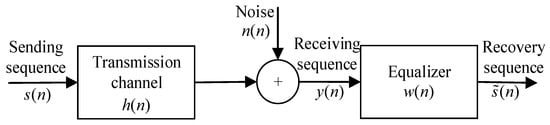
Figure 1.
Blind equalization system model.
Where is the sending sequence, is the impulse response of the discrete time transmission channel, is the superimposed noise on the channel, such as Gaussian white noise, and is the receiving sequence. The specific formula is shown in Equation (18). The impulse response of the blind equalizer is ; is the length of the equalizer; and is the recovery sequence of the blind equalization system.
where represents convolution, .
3.2. Basic Principle of CMA
The CMA was one of the most widely studied algorithms in blind equalization because of its simple structure, strong practicability and excellent performance [41]. However, in the process of equalization, the constant modulus algorithm also has the disadvantages of falling into local optimal and being unable to jump out, having a slow convergence rate and requiring more signal points for iteration [42]. The whole system structure is formed by adding Gaussian white noise to the input sequence after passing through the channel . The is an input sequence in equalizer to get the estimated sequence . Finally, the decision sequence is generated by the decision device. The principal diagram of the CMA is shown in Figure 2.
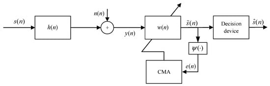
Figure 2.
The principal diagram of the CMA.
Where is the error generating function, is the error function of constant modulus algorithm, is the decision value of recovery sequence obtained by the decision device.
where is the length of a finite-length transverse filter, is the length of channel. represents the transpose of the matrix.
The error function of CMA is as follows:
The cost function of CMA is as follows:
The updated formula of weight of CMA algorithm is obtained by using the fastest descent method:
where is the step of the iteration, is the instantaneous value after taking the partial derivative. The specific formula is as follows.
where is conjugate of the recovery sequence, is the conjugate of the input signal of the equalizer.
3.3. The Constant Modulus Blind Equalization Algorithm Based on Hybrid Arithmetic Whale Optimization
Because of the slow convergence speed and strong randomness of initial weights of the CMA, a hybrid arithmetic whale constant modulus blind equalization algorithm (HAWOA-CMA) is designed in this section. The schematic diagram of the HAWOA-CMA system is shown in Figure 3. The received sequence is taken as the input signal of the HAWOA algorithm, and the mean square error of the whole equalization system is set as the cost function of HAWOA. The formula is shown in Equations (31) and (32).
where represent the number of iteration points, is the mean square error, is the fitness of HAWOA.
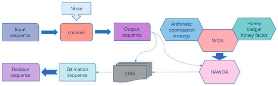
Figure 3.
Schematic Diagram of the HAWOA-CMA.
In HAWOA, the individual whale corresponds to the weight vector of the equalizer, and the MSE is taken as the cost function. In the iteration process, the minimum value of the cost function is found by updating the position of each whale. Therefore, a group of optimal whale positions under the condition of minimum fitness value is obtained. Then the optimal whale position is regarded as the initial weight value assigned to the optimal weight vector in the CMA equalizer. Finally, the optimal estimation sequence is obtained by iteration and decision. The specific process of HAWOA-CMA is shown in Algorithm 1. The schematic flowchart of HAWOA-CMA is shown in Figure 4.
| Algorithm 1. The process of HAWOA-CMA algorithm |
| 1: Initializing the step size |
| 2: Initializing the whale position and using the MSE of CMA to initialize the cost function of HAWOA |
| 3: Obtaining the weight vector with minimum fitness by taking the iteration calculating of HAWOA |
| 4: Defining the weight vector obtained from HAWOA as the initial weight vector of HAWOA-CMA |
| 5: Using the Equation (21) to calculate the output sequence of equalizer |
| 6: Using the Equation (23) to calculate the error |
| 7: Using the Equation (26) to update the weight |
| 8: Calculating the MSE |
| 9: Determine whether the end condition has been met, if so, proceed to step 10, if not, return to step 4 |
| 10: End |
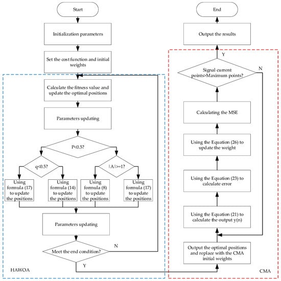
Figure 4.
The schematic flowchart of HAWOA-CMA.
4. Experiment and Discussion
4.1. Validity Analysis
To demonstrate the suitability of the HAWOA for addressing the constant modulus blind equalization problem, this section analyzes the advantages of HAWOA compared to other algorithms from the perspective of test functions. The effectiveness of the algorithm is further analyzed through test data. Therefore, an analysis of the cost function to CMA is conducted, and experiments are designed to verify the applicability and validity of the cost function. In this section, the popular optimization algorithms were selected for comparison, including the Harris hawks optimization algorithm (HHO), butterfly optimization algorithm [43] (BOA), seagull optimization algorithm [44] (SOA), Aquila optimizer (AO), arithmetic optimization algorithm (AOA) and WOA. The minimum distribution of the CMA cost function is shown in Figure 5.
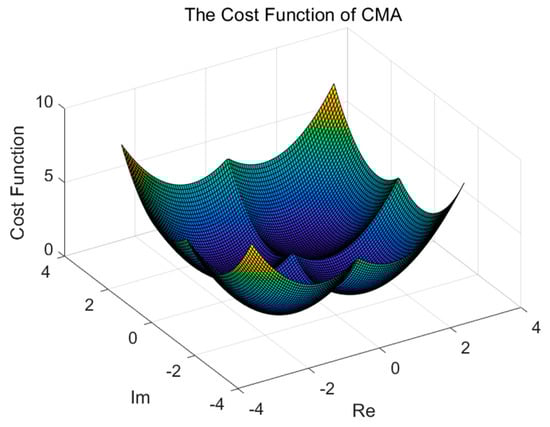
Figure 5.
The minimum distribution of the CMA cost function.
Based on the cost function and the distribution of global minima in the CMA, it can be observed that the distribution of global minima is similar to the bowl-shaped, plate-shaped and valley-shaped functions. Therefore, this subset of test functions are employed to conduct experiments on HAWOA, aiming to validate its effectiveness and applicability further. Detailed information on the test functions is presented in Table 1.

Table 1.
The bowl-shaped, plate-shaped and valley-shaped test functions.
Where the Range and dim respectively represent the definition domain and dimension. The shape of function is shown in Figure 6.
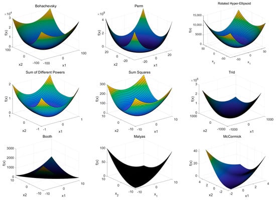
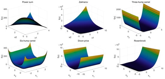
Figure 6.
The shape of bowl-shaped, plate-shaped and valley-shaped test functions.
Where are the bowl-shaped functions, are the plate-shaped functions and are the valley-shaped functions. The results of HAWOA and other comparison algorithms on are shown in Table 2.
Table 2.
The results on bowl-shaped, plate-shaped and valley-shaped functions.
As listed in Table 2, it can be observed that HAWOA has the highest overall ranking, while WOA has the fifth overall ranking. In the case of bowl-shaped, plate-shaped and valley-shaped test functions, HAWOA shows a certain superiority over other comparative algorithms. It has been verified experimentally that the improvement strategies employed in HAWOA effectively enhance the search performance of the WOA.
Figure 7 depicts the convergence curves of HAWOA and other comparative algorithms when tested on . According to the comparison, it is evident that the curve of HAWOA exhibits a lower slope, allowing it to achieve smaller optimization values within a shorter number of iterations. In function F1, HAWOA demonstrates significantly faster convergence speed than other algorithms, proving its excellent optimization performance in dealing with bowl-shaped cost functions, which are characterized by a distribution of local minima in a bowl shape. Furthermore, HAWOA maintains its leading position in terms of convergence speed when tested on plate-shaped and valley-shaped functions. Combining the convergence ranking results in Table 2, HAWOA outperforms the comparative algorithms regarding overall optimization performance. This experiment tests the optimization performance of HAWOA using bowl-shaped, plate-shaped and valley-shaped functions, which bear similarities to the cost function in constant modulus blind equalization problems. These results indirectly demonstrate the promising performance of HAWOA in solving blind equalization problems.
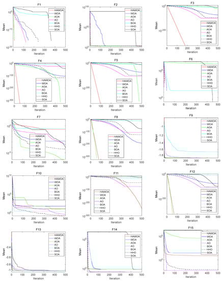
Figure 7.
The convergence curves of the bowl-shaped, plate-shaped and valley-shaped functions.
4.2. Test and Analysis of HAWOA-CMA
In this section, 16QAM and 64QAM were used to test the HAWOA-CMA system. Five hundred Monte Carlo experiments were conducted, respectively. CMA and WOA-CMA were used as comparison objects for simulation. The channel parameters are h = [0.9656, −0.0906, 0.0578, 0.2368]; the signal-to-noise ratio was 20 dB; and the length of the equalizer weight was 16. The initial weight of the CMA is set by experience, with the eighth tap coefficient set to 1 and the remaining tap coefficient set to 0. The input weights of WOA-CMA and HAWOA-CMA are set as random values between [−1,1].
4.2.1. The Sending Sequence Is 16QAM
When the HAWOA-CMA system sends 16QAM signals with a sequence of 10,000 points, the step size is , and , respectively. WOA and HAWOA populations were 50, and the maximum number of iterations was 50. The experimental results are shown in Figure 8.
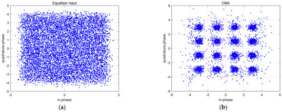
Figure 8.
Constellation of equalizer input and output at 16QAM signal (a) Input (b) CMA (c) WOA (d) HAWOA.
In Figure 8, Figure 8a is the input sequence constellation diagram of the equalizer. The red point is the phase point of the 16QAM signal. Due to the influence of channel and noise, the input signal becomes disordered and divergent, which does not conform to the optimal constellation structure of the 16QAM signal. Figure 8b is the signal constellation diagram after equalization by the constant modulus algorithm. The balanced points can be close to the optimal constellation structure of 16QAM on a macro level. However, many divergence points have a larger amplitude, and its equilibrium performs imperfectly. Figure 8c,d are signal constellation figures after WOA-CMA and HAWOA-CMA equalization. It should be noted that two balanced signal points converge to the optimal constellation structure of 16QAM, and there are fewer divergence points and no points with larger amplitude compared to Figure 8b. This difference is because the CMA has a slow convergence in the equalization process, and it is difficult to obtain the equalizer weight suitable for the unknown channel in a short iteration. Before getting the suitable equalizer weight, the equalization performs poorly, so some diverging points with large amplitude will be generated. In other words, WOA-CMA and HAWOA-CMA can quickly obtain better equalizer weights, and the equalization effect is better than CMA. The MSE is shown in Figure 9.
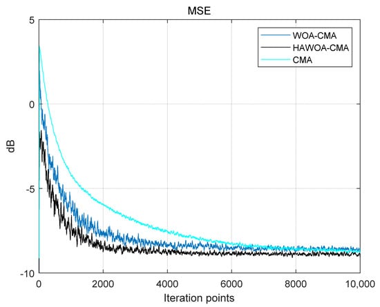
Figure 9.
16QAM signal mean square error.
Where the abscissa represents the number of iteration points of the blind equalization algorithm, and the ordinate is the size of MSE. The initial MSE of WOA-CMA and HAWOA-CMA is smaller than CMA, and HAWOA-CMA has a smaller number of iteration points when reaching the same convergence value. Compared with the CMA and WOA-CMA, it can reduce nearly 1000 and 300 iterations under the same mean square error condition. It can be proven that HAWOA-CMA has a faster convergence rate and can get a convergence value in the shortest time.
WOA-CMA and HAWOA-CMA have substantial advantages over CMA in equalization effect. However, using a swarm intelligence algorithm to optimize blind equalization will bring some problems, such as increased computation and longer computation time. Therefore, reducing the number of iterations of the swarm intelligence algorithm to achieve the same equalization effect becomes the key to effectively reducing the computation amount and time. As mentioned in Section 4.1, HAWOA has a faster convergence speed and better accuracy than WOA. To reflect the superiority of HAWOA in blind equalization, the number of iterations obtained by the algorithm in the optimization process of WOA-CMA and HAWOA-CMA initialization weights was recorded. Figure 10 shows the boxplot of the number of iterations when WOA and HAWOA find the optimal solution in 500 Monte Carlo experiments.
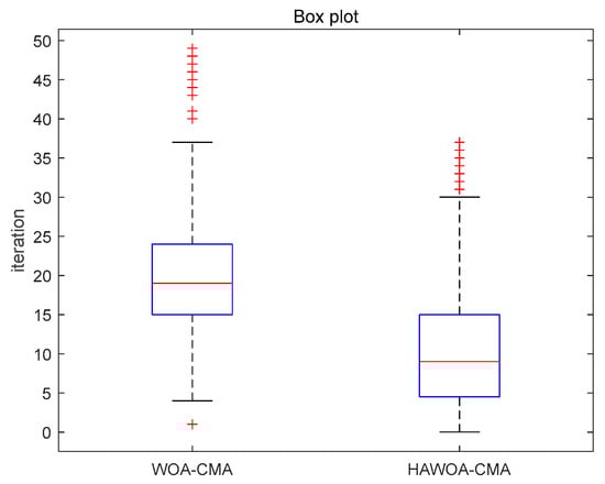
Figure 10.
Boxplot of the number of iterations in 16QAM.
According to Figure 10, the ordinate is the iterations of the algorithm. According to the analysis of boxplot properties [45], the iterations of HAWOA-CMA are generally small, and the upper limit and lower limit are lower than WOA-CMA. The extreme outliers are less than WOA-CMA, indicating that HAWOA-CMA has more substantial stability and better performance than WOA-CMA. The average iterations of WOA-CMA and HAWOA-CMA were 20.57 and 11.12, respectively. Therefore, it can be concluded that HAWOA-CMA uses fewer iterations, which can effectively reduce the calculation amount and time compared with WOA-CMA.
The Figure 11 below illustrates the comparison of the symbol error rate (SER) of the model under different signal-to-noise ratio (SNR) conditions. It can be observed that both WOA-CMA and HAWOA-CMA have lower BER than CMA under the same SNR. When the SNR is 20 dB, the SER of the WOA-CMA system is approximately −35 dB, while the SER of the HAWOA-CMA system is around −40 dB. The difference between the two is approximately 5 dB, indicating that the blind equalization system incorporating HAWOA has a lower SER compared to the system incorporating WOA. Furthermore, when the SNR is 25 dB and 30 dB, both WOA-CMA and HAWOA-CMA systems exhibit a linear SER value of 0 while the SER of the CMA system remains between −20 dB and −25 dB. This further confirms that the model effectively reduces the SER of the traditional CMA system in the channel equalization process. Additionally, the HAWOA-CMA model requires a lower SNR to achieve the same SER, making it more suitable for wireless communication environments with higher noise power.
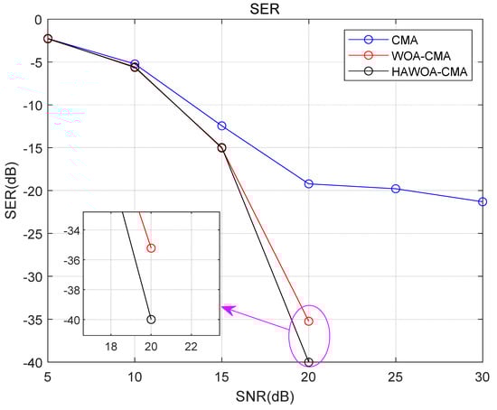
Figure 11.
The SER in 16QAM.
4.2.2. The Sending Sequence Is 64QAM
When the HAWOA-CMA system sends 64QAM signals with a sequence of 10,000 points, the step size is , and , respectively. WOA and HAWOA populations were 50, and the maximum number of iterations was 50.
In Figure 12, Figure 12a is the input sequence constellation diagram of the equalizer. The red point is the phase point of the 64QAM signal. Figure 12b is the signal constellation diagram after equalization by the constant modulus algorithm. It is worth mentioning here that the balanced points can be close to the optimal constellation structure of 64QAM on a macro level. However, there are still more divergence points and some points have larger amplitude. Figure 12c,d are signal constellation figures after WOA-CMA and HAWOA-CMA equalization. Meanwhile, the two balanced signal points converge to the optimal constellation structure of 64QAM, and there are fewer divergence points and no points with larger amplitude compared to Figure 12b. It is further proven that WOA-CMA and HAWOA-CMA can quickly obtain appropriate equalizer weights, and the equalization effect is very competitive compared to CMA. Its mean square error is shown in Figure 13.
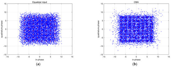
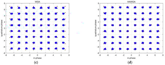
Figure 12.
Constellation of equalizer input and output at 64QAM signal (a) Input (b) CMA (c) WOA (d) HAWOA.
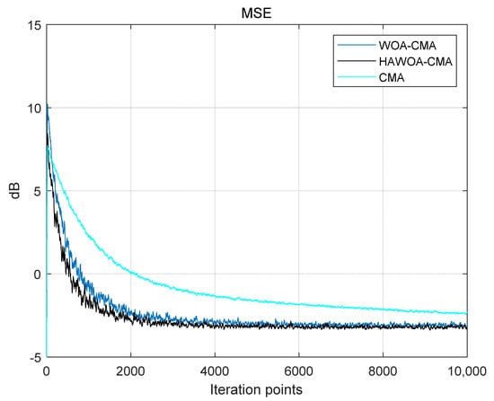
Figure 13.
64QAM signal mean square error.
It can be seen from Figure 13 that HAWOA-CMA has a smaller number of iteration points when reaching the same convergence value, maintaining the fastest convergence rate. Compared with the CMA and WOA-CMA, it can reduce nearly 1500 and 300 iterations under the same mean square error condition. It is proven that HAWOA-CMA still has an excellent balancing performance when the input signal is 64QAM. Figure 14 shows the boxplot of the iterations of WOA and HAWOA in the 64QAM signal.
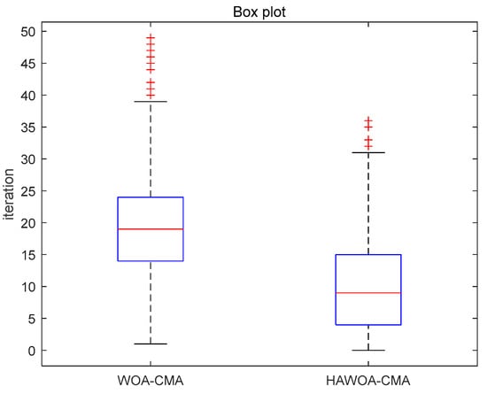
Figure 14.
Boxplot of the number of iterations in 64QAM.
As depicted in Figure 14, the iterations of HAWOA-CMA are relatively small, and the upper limit and lower limit are lower than WOA-CMA. The extreme outliers were far less than WOA-CMA. The average number of iterations was 20.21 for WOA-CMA and 10.38 for HAWOA-CMA. The figure proves that HAWOA-CMA has a faster optimization speed and notably outperforms WOA-CMA.
In Figure 15, similarly, when the input signal of the equalization system is 64QAM, both WOA-CMA and HAWOA-CMA exhibit lower SER than CMA under different SNR conditions, with HAWOA-CMA demonstrating superior SER performance compared to CMA. When the SNR is 25 dB, the SER of HAWOA-CMA is lower than that of WOA-CMA, with a difference of approximately 3 dB. Combining the analysis of MSE, HAWOA-CMA achieves faster convergence speed while maintaining preferable SER performance. In contrast, the traditional CMA exhibits poor equalization performance and higher SER when the input is a higher-order QAM signal. Compared to CMA, the proposed model effectively reduces the SER of the equalization system in wireless communication, mitigating the impact of channel and noise to improve communication quality.
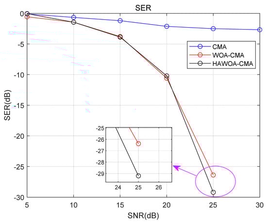
Figure 15.
The SER in 64QAM.
4.2.3. Result Analysis and Contribution of HAWOA-CMA
The QAM signal is commonly used in wireless communication systems due to its high data transmission rate, spectral efficiency and good noise resistance. To evaluate the performance of HAWOA-CMA in wireless communication systems, this study conducted simulation tests using both 16QAM and 64QAM signals. Based on the simulation data, it was observed that HAWOA-CMA demonstrated faster convergence, minor mean square error and lower bit error rate compared to the original method for both 16QAM and 64QAM input signals. These improvements indicate that HAWOA-CMA enhances the performance of the equalizer to a certain extent. In wireless communication systems, faster convergence improves real-time capability and resistance to interference while a lower bit error rate enhances communication quality and system reliability. The performance above enhancements signifies that the HAWOA-CMA model can improve the equalization effectiveness and elevate data transmission quality and system stability in wireless communication systems.
Additionally, this study combines channel equalization with metaheuristic algorithms from artificial intelligence, offering valuable insights into integrating wireless communication systems with artificial intelligence.
5. Conclusions
In this study, based on the idea of AI-assisted channel estimation, a hybrid arithmetic whale constant modulus blind equalization algorithm is proposed as an effective channel equalization method. By improving the blind equalization algorithm, the advantages in fast time-varying channels are given full play. The novelty of this research lies in using swarm intelligence algorithms with substantial population diversity to address practical channel equalization problems. By incorporating a hybrid approach, the deficiencies of the whale optimization algorithm are addressed, providing a viable approach to enhance the blind equalization systems in wireless channels through the integration of artificial intelligence. In the process of experiment, firstly, the new swarm intelligence algorithms in recent years are compared to illustrate the effectiveness of the HAWOA, and the applicability of the algorithm is verified according to the characteristics of the CMA cost function. Secondly, the simulation is carried out with the CMA and the WOA-CMA under the input signal of 16QAM and 64QAM, respectively. The results show that the HAWOA has a preferable optimization performance and obvious advantages in comparison. It can be regarded as an efficient optimization method for solving bowl-shaped optimization problems. In the channel equalization process, HAWOA-CMA has a faster convergence speed and better convergence accuracy than CMA and WOA-CMA. In the initial weight optimization process, HAWOA-CMA can obtain the weight with a smaller fitness value and fewer iterations. Compared with the classical method, HAWOA-CMA can converge quickly and effectively reduce the mean square error. The computation amount and time of the equilibrium system are reduced while keeping the time and space complexity unchanged. This method can perfectly improve communication efficiency under the time-varying channel and ensure a low SER, reduce bandwidth consumption and enhance the equalization effect.
This finding will facilitate further investigation into applying the swarm intelligence algorithm in blind equalization. The convergence speed of this model still needs to be improved, and the optimization method still has some stability problems. Future research can be aimed at using a more stable optimization method to solve the blind equalization problem. At the same time, applying the popular deep learning method to the optimization of the constant modulus blind equalization system also has a certain research value.
Author Contributions
Conceptualization, Writing—original draft, X.W.; Methodology, L.Z.; Writing—review and editing, Y.S.; Project administration, Y.Z.; Software, Y.H. All authors have read and agreed to the published version of the manuscript.
Funding
The study is subsidized by Tianjin Research Innovation Project for Postgraduate Students (No.2021YJSS293).
Data Availability Statement
Not applicable.
Acknowledgments
The authors would like to thank the laboratory and university for their support.
Conflicts of Interest
The authors declare that the research was conducted in the absence of any commercial or financial relationships that could be construed as a potential conflict of interest.
References
- Liang, Y.; Gao, N.; Liu, T. Suppression method of inter-symbol interference in communication system based on mathematical chaos theory. J. King Saud. Univ. Sci. 2020, 32, 1749–1756. [Google Scholar] [CrossRef]
- Ren, H.P.; Yin, H.P.; Zhao, H.E.; Bai, C.; Grebogi, C. Artificial intelligence enhances the performance of chaotic baseband wireless communication. IET Commun. 2021, 15, 1467–1479. [Google Scholar] [CrossRef]
- Yin, C.J.; Feng, W.J.; Li, G.J. Improved soft-decision feedback turbo equalization algorithm with dual equalizers. Int. J. Electron. Commun. 2022, 157, 154436. [Google Scholar] [CrossRef]
- Zhang, M.H.; Wang, Y.F.; Tu, X.B.; Qu, F.Z.; Zhao, H.F. Recursive Least Squares-Algorithm-Based Normalized Adaptive Minimum Symbol Error Rate Equalizer. IEEE Commun. Lett. 2023, 27, 319–321. [Google Scholar] [CrossRef]
- Lee, S.M.; Min, M. Convexity of the Capacity of One-Bit Quantized Additive White Gaussian Noise Channels. Mathematics 2022, 10, 4343. [Google Scholar] [CrossRef]
- Liu, B.Y.; Gong, C.; Cheng, J.L.; Xu, Z.Y.; Liu, J.J. Blind and Semi-Blind Channel Estimation/Equalization for Poisson Channels in Optical Wireless Scattering Communication Systems. IEEE Trans. Wirel. Commun. 2022, 21, 5930–5946. [Google Scholar] [CrossRef]
- Fan, K.G.; Hou, H.N.; Tang, Y.F.; Liu, P.C. Orthogonality constrained analytic CMA for blind signal extraction improvement. Signal Process. 2023, 205, 108880. [Google Scholar] [CrossRef]
- Peken, T.; Vanhoy, G.; Bose, T. Blind channel estimation for massive MIMO. Analog Integr. Circuits Signal Process. 2017, 91, 257–266. [Google Scholar] [CrossRef]
- Yang, L.; Han, Q.; Du, J.; Cheng, L.; Li, Q.Q.; Zhao, A. Online Blind Equalization for QAM Signals Based on Prediction Principle via Complex Echo State Network. IEEE Commun. Lett. 2020, 24, 1338–1341. [Google Scholar] [CrossRef]
- Yu, X.; Liu, W.; Xie, J.; Xu, M.; Li, H.; Zhang, Q.; Xu, C.; Hu, S.R.; Huang, D.Q. Characterization of Low-Power Wireless Links in UAV-Assisted Wireless-Sensor Network. IEEE Internet Things J. 2023, 10, 5823–5842. [Google Scholar]
- Li, X.Q.; Feng, G.; Liu, Y.J.; Qin, S.; Zhang, Z.P. Joint Sensing, Communication, and Computation in Mobile Crowdsensing Enabled Edge Networks. IEEE Trans. Wirel. Commun. 2022, 22, 2818–2832. [Google Scholar] [CrossRef]
- Ashraf, M.; Tan, B.; Moltchanov, D.; Thompson, J.S.; Valkama, M. Joint Optimization of Radar and Communications Performance in 6G Cellular Systems. IEEE Trans. Green Commun. Netw. 2023, 7, 522–536. [Google Scholar] [CrossRef]
- Johnson, R.; Schniter, P.; Endres, T.J.; Behm, J.D.; Brown, D.R.; Casas, R.A. Blind equalization using the constant modulus criterion: A review. Proc. IEEE Inst. Electr. Electron. Eng. 1998, 86, 1927–1950. [Google Scholar] [CrossRef]
- Ahmed, S.; Khan, Y.; Wahab, A. A Review on Training and Blind Equalization Algorithms for Wireless Communications. Wirel. Pers. Commun. 2019, 108, 1759–1783. [Google Scholar] [CrossRef]
- Benveniste, A.; Goursat, M. Blind Equalizers. IEEE Trans. Commun. 1984, 32, 871–883. [Google Scholar] [CrossRef]
- Yang, J.; Werner, J.J.; Durmont, G.A. The multimodulus blind equalization and its generalized algorithms. IEEE J. Sel. Areas Commun. 2002, 20, 997–1015. [Google Scholar] [CrossRef]
- Chang, W.C.; Yuan, J.T. CMA adaptive equalization in subspace pre-whitened blind receivers. Digit. Signal Process. 2019, 88, 33–40. [Google Scholar] [CrossRef]
- Ma, J.T.; Qiu, T.S.; Tian, Q. Fast Blind Equalization Using Bounded Non-Linear Function With Non-Gaussian Noise. IEEE Commun. Lett. 2020, 24, 1812–1815. [Google Scholar] [CrossRef]
- Li, J.; Li, G.; Xie, H.; Li, Q. Low-complexity Gaussian-Newton method for mutimodulus algorithm-based blind equalization. Signal Process. 2022, 201, 108722. [Google Scholar] [CrossRef]
- Sun, J.Q.; Li, X.G.; Chen, K.; Cui, W.; Chu, M. A Novel CMA+DD_LMS Blind Equalization Algorithm for Underwater Acoustic Communication. Comput. J. 2020, 63, 974–981. [Google Scholar] [CrossRef]
- Zhang, Y.J.; Tian, S.L.; Pan, H.Q.; Zhang, Q.C.; Qiu, D.Y.; Zhou, Y. Adaptive blind equalization for multi-level QAM signals in impulsive noise environment. IET Commun. 2022, 16, 314–325. [Google Scholar] [CrossRef]
- Khafaji, M.J.; Krasicki, M. Uni-Cycle Genetic Algorithm to Improve the Adaptive Equalizer Performance. IEEE Commun. Lett. 2021, 25, 3609–3613. [Google Scholar] [CrossRef]
- Zhang, Z.; Zhang, J.H.; Zhang, Y.X.; Li, Y.; Liu, G.Y. AI-Based Time-, Frequency-, and Space-Domain Channel Extrapolation for 6G: Opportunities and Challenges. IEEE Veh. Technol. Mag. 2023, 18, 29–39. [Google Scholar] [CrossRef]
- Tang, J.; Liu, G.; Pan, Q.T. A Review on Representative Swarm Intelligence Algorithms for Solving Optimization Problems: Applications and Trends. IEEE-CAA J. Autom. 2021, 8, 1627–1643. [Google Scholar] [CrossRef]
- Xu, T.T.; Xiang, Z. Modified constant modulus algorithm based on bat algorithm. J. Intell. Fuzzy Syst. 2021, 41, 4493–4500. [Google Scholar] [CrossRef]
- Zhang, R.; Chen, C.K.; Pan, C.S. Chaos Chicken Swarm-based Blind Equalization Algorithm for Multipath Mitigation of UAVs. In Proceedings of the 2021 6th International Symposium on Computer and Information Processing Technology, Changsha, China, 23 December 2021; pp. 268–289. [Google Scholar]
- Mirjalili, S.; Lewis, A. The Whale Optimization Algorithm. Adv. Eng. Softw. 2016, 95, 51–67. [Google Scholar] [CrossRef]
- Mavorvouniotis, M.; Li, C.H.; Yang, S.X. A survey of swarm intelligence for dynamic optimization: Algorithms and applications. Swarm Evol. Comput. 2017, 33, 1–17. [Google Scholar] [CrossRef]
- Wang, D.S.; Tan, D.P.; Liu, L. Particle swarm optimization algorithm: An overview. Soft Comput. 2018, 22, 387–408. [Google Scholar] [CrossRef]
- Akbari, R.; Hedayatzadeh, R.; Ziarati, K.; Hassanizadeh, B. A multi-objective artificial bee colony algorithm. Swarm Evol. Comput. 2012, 2, 39–52. [Google Scholar] [CrossRef]
- Heidari, A.A.; Mirjalili, S.; Faris, H.; Aljarah, I.; Mafarja, M.; Chen, H.L. Harris hawks optimization: Algorithm and applications. Future Gener. Comput. Syst. 2019, 97, 849–872. [Google Scholar] [CrossRef]
- Abualigah, L.; Yousri, D.; Elaziz, M.A.; Fwees, A.A.; Al-qaness, M.A.A.; Gandomi, A.H. Aquila Optimizer: A novel meta-heuristic optimization algorithm. Comput. Ind. Eng. 2021, 157, 107250. [Google Scholar] [CrossRef]
- Wang, C.H.; Chen, S.M.; Zhao, Q.G.; Suo, Y.F. An Efficient End-to-End Obstacle Avoidance Path Planning Algorithm for Intelligent Vehicles Based on Improved Whale Optimization Algorithm. Mathematics 2023, 11, 1800. [Google Scholar] [CrossRef]
- Ling, Y.; Zhou, Y.Q.; Luo, Q.F. Levy Flight Trajectory-Based Whale Optimization Algorithm for Global Optimization. IEEE Access 2017, 5, 6168–6186. [Google Scholar] [CrossRef]
- Jiang, R.K.; Wang, X.T.; Cao, S.; Zhao, J.F.; Li, X.R. Joint Compressed Sensing and Enhanced Whale Optimization Algorithm for Pilot Allocation in Underwater Acoustic OFDM Systems. IEEE Access 2019, 7, 95779–95796. [Google Scholar] [CrossRef]
- Paul, K.; Shekher, V.; Kumar, N.; Kumar, V.; Kumar, M. Influence of Wind Energy Source on Congestion Management in Power System Transmission Network: A Novel Modified Whale Optimization Approach. Proc. Integr. Optim. 2022, 6, 943–959. [Google Scholar] [CrossRef]
- Zhang, M.G.; Zhang, F.X.; Gao, Y.X. The optimal scheduling of microgrid: A research based on a novel whale algorithm. Energy Rep. 2023, 9, 894–903. [Google Scholar] [CrossRef]
- Gharehchopogh, F.S.; Gholizadeh, H. A comprehensive survey: Whale Optimization Algorithm and its applications. Swarm Evol. Comput. 2019, 48, 1–24. [Google Scholar] [CrossRef]
- Abualigah, L.; Diabat, A.; Mirjalili, S.; Elaziz, M.A.; Gandomi, A.H. The Arithmetic Optimization Algorithm. Comput. Methods Appl. Mech. Eng. 2021, 376, 113609. [Google Scholar] [CrossRef]
- Hashim, F.A.; Houssein, E.H.; Hussain, K.; Mabrouk, M.S.; Al-Atabany, W. Honey Badger Algorithm: New metaheuristic algorithm for solving optimization problems. Math. Comput. Simul. 2022, 192, 84–110. [Google Scholar] [CrossRef]
- Abrar, S.; Nandi, A.K. An Adaptive Constant Modulus Blind Equalization Algorithm and Its Stochastic Stability Analysis. IEEE Signal Process. Lett. 2010, 17, 55–58. [Google Scholar] [CrossRef]
- Sung, W.T. Wireless sensing network transmission system with improved constant modulus algorithm. EURASIP J. Wirel. Commun. Netw. 2013, 2013, 1–8. [Google Scholar] [CrossRef]
- Arora, S.; Singh, S. Butterfly optimization algorithm: A novel approach for global optimization. Soft Comput. 2019, 23, 715–734. [Google Scholar] [CrossRef]
- Dhiman, G.; Kumar, V. Seagull optimization algorithm: Theory and its applications for large-scale industrial engineering problems. Knowl. Based Syst. 2019, 165, 169–196. [Google Scholar] [CrossRef]
- Lem, S.; Onghena, P.; Verschaffei, L.; Dooren, W.V. The heuristic interpretation of box plots. Learn. Instr. 2013, 26, 22–35. [Google Scholar] [CrossRef]


Disclaimer/Publisher’s Note: The statements, opinions and data contained in all publications are solely those of the individual author(s) and contributor(s) and not of MDPI and/or the editor(s). MDPI and/or the editor(s) disclaim responsibility for any injury to people or property resulting from any ideas, methods, instructions or products referred to in the content. |
© 2023 by the authors. Licensee MDPI, Basel, Switzerland. This article is an open access article distributed under the terms and conditions of the Creative Commons Attribution (CC BY) license (https://creativecommons.org/licenses/by/4.0/).