A Bimodal Extension of the Log-Normal Distribution on the Real Line with an Application to DNA Microarray Data

Abstract

A bimodal double log-normal distribution on the real line is proposed using the random sign mixture transform. Its associated statistical inferences are derived. Its parameters are estimated by the maximum likelihood method. The performance of the estimators and the corresponding confidence intervals is checked by simulation studies. Application of the proposed distribution to a real data set from a DNA microarray is presented.

1. Introduction

A log-normal distribution is perhaps the most popular model for skewed data [1]. However, a log-normal distribution is defined only on the positive real line. Many of its application areas involve data spanning the entire real line. One example is the modeling of stock returns. The log-normal distribution is a popular model for stock returns. However, stock returns can be positive or negative. Positive stock returns correspond to profits, while negative stock returns correspond to losses. Other application areas of log-normal distributions involving data spanning the entire real line are discussed later on. Hence, a double log-normal distribution is needed.

We follow the procedure presented in [2] to construct a double log-normal (DLN) distribution. Consider the following two transforms [2]:

(i)

The random sign transform (RST) given by

$$\begin{array}{c}\hfill {\displaystyle W=(2Y-1)X;}\end{array}$$

(ii)

The random sign mixture transform (RSMT) given by

$$\begin{array}{c}\hfill {\displaystyle Z=Y{X}_1-(1-Y)X_2,}\end{array}$$

where Y is a Bernoulli random variable (RV) with parameter $\beta$ and X, $X_1$ and $X_2$ are non-negative RVs independent of Y. The probability density function (PDF) of W is

$$\begin{array}{c}\hfill {\displaystyle f_W\left(w;\beta ,\mathit{\theta }\right)=\left\{\begin{array}{cc}{\displaystyle \overline{\beta }{f}_X\left(\left|w\right|;\mathit{\theta }\right),}\hfill & w<0,\hfill \\ {\displaystyle \beta f_X\left(w;\mathit{\theta }\right),}\hfill & w\ge 0,\hfill \end{array}\right.}\end{array}$$

and the PDF of Z is

$$\begin{array}{c}\hfill {\displaystyle f_Z\left(z;\beta ,{\mathit{\theta }}_1,{\mathit{\theta }}_2\right)=\left\{\begin{array}{cc}{\displaystyle \overline{\beta }{f}_{X_2}\left(\left|z\right|;{\mathit{\theta }}_2\right),}\hfill & z<0,\hfill \\ {\displaystyle \beta f_{X_1}\left(z;{\mathit{\theta }}_1\right),}\hfill & z\ge 0,\hfill \end{array}\right.}\end{array}$$

where $f_X\left(·;\mathit{\theta }\right)$, $f_{X_1}\left(·;{\mathit{\theta }}_1\right)$, $f_{X_2}\left(·;{\mathit{\theta }}_2\right)$ are the PDFs of non-negative RVs X, $X_1$ and $X_2$, respectively, with (vector) parameters $\mathit{\theta }$, ${\mathit{\theta }}_1$ and ${\mathit{\theta }}_2$, respectively. If X is an RV from a family of distributions ${\mathcal{F}}_1$, then W is said to have a double ${\mathcal{F}}_1$ distribution. If $X_1$ and $X_2$ are independent RVs from a family of distributions ${\mathcal{F}}_2$, then Z is said to have a double${\mathcal{F}}_2$ distribution.

There are many double continuous distributions on the real line. However, the words ‘double’ or ‘reflection’ are sometimes used to denote the distribution of the absolute value of a random variable. Some double continuous distributions based on the RST are:

• Double exponential distribution (Laplace) [3].
• Double generalized gamma distribution [4].
• Double Weibull distribution [5].
• Double gamma distribution [6].
• Double generalized Pareto distribution [7].
• Double Lomax distribution [8].
• Double Lindley distribution [9].

Some double continuous distributions based on the RSMT are:

• Double half-normal distribution [10,11].
• Double exponential distribution [12].
• Double inverse gamma distribution [13].
• Double Gompertz distribution [14].
• Double Pareto II distribution [15].
• Double inverse Gaussian distribution [16].

We construct the DLN distribution using the RSMT, i.e., the distribution of Z when $X_1$ and $X_2$ independently follow the log-normal distribution.

The remainder of this paper is organized as follows. In Section 2, the statistical properties of the DLN distribution are presented. The maximum likelihood estimates (MLEs) of the parameters and their asymptotic distributions are studied in Section 3. Simulations to check the finite sample performance of the estimators of the parameters and the corresponding confidence intervals are presented in Section 4. An application of the proposed double distribution to a real data set from a DNA microarray is presented in Section 5. Finally, the conclusions and comments are stated in Section 6.

2. Statistical Properties

We present the statistical properties of the DLN distribution in this section.

2.1. Probability Density Function

The PDF of the DLN distribution is

$$\begin{array}{c}\hfill {\displaystyle f_Z\left(z\right)=\left\{\begin{array}{cc}{\displaystyle \overline{\beta }{f}_{X_2}\left(\left|z\right|;{\mu }_2,{\sigma }_2\right),}\hfill & z<0,\hfill \\ {\displaystyle \beta f_{X_1}\left(z;{\mu }_1,{\sigma }_1\right),}\hfill & z\ge 0,\hfill \end{array}\right.}\end{array}$$

where for $-\infty <{\mu }_1,{\mu }_2<\infty$ and ${\sigma }_1,{\sigma }_2>0$, and

$$\begin{array}{c}\hfill {\displaystyle f_{X_j}\left(x;{\mu }_j,{\sigma }_j\right)=\frac{1}{\sqrt{2\pi }\sigma x}exp\left[-\frac{{\left(ln\left(x\right)-{\mu }_j\right)}^2}{2{\sigma }_j^2}\right],x>0,j=1,2}\end{array}$$

(1)

are the PDFs of the LN distributions.

Figure 1 shows the bimodality of the PDF of the DLN distribution for selected parameter values.

Figure 1. PDF of the DLN distribution: $\left(\beta , {\mu }_1, {\sigma }_1, {\mu }_2, {\sigma }_2\right)$: (0.3, −0.5, 1, 0.5, 1) (), (0.5, −0.5, 1, 0.5, 1) (), $(0.8, -0.5, 1, 0.5, 1)$ ().

The DLN distribution has two modes given by

$$\begin{array}{c}\hfill {\displaystyle \mathrm{Mode}\left(Z\right)=-\mathrm{Mode}\left(X_2\right)\mathrm{and}\mathrm{Mode}\left(X_1\right),}\end{array}$$

where

$$\begin{array}{c}\hfill {\displaystyle \mathrm{Mode}\left(X_j\right)=e^{{\mu }_j-{\sigma }_j^2},j=1,2}\end{array}$$

(2)

are the modes of the LN distributions.

2.2. Cumulative Distribution Function

The cumulative distribution function (CDF) of the DLN distribution is

$$\begin{array}{c}\hfill {\displaystyle F_Z\left(z\right)=P(Z\le z)=\left\{\begin{array}{cc}{\displaystyle \overline{\beta }\left[1-F_{X_2}\left(\left|z\right|;{\mu }_2,{\sigma }_2\right)\right],}\hfill & z<0,\hfill \\ {\displaystyle \overline{\beta }+\beta F_{X_1}\left(z;{\mu }_1,{\sigma }_1\right),}\hfill & z\ge 0,\hfill \end{array}\right.}\end{array}$$

(3)

where

$$\begin{array}{c}\hfill {\displaystyle F_{X_j}\left(x;{\mu }_j,{\sigma }_j\right)=P\left(X_j\le x\right)=\Phi \left(\frac{ln\left(x\right)-{\mu }_j}{{\sigma }_j}\right),x>0,j=1,2}\end{array}$$

are the CDFs of the LN distributions and

$$\begin{array}{c}\hfill {\displaystyle \Phi \left(a\right)=P(Z\le a)={\int }_{-\infty }^a\frac{1}{\sqrt{2\pi }}{e}^{-z^2/2}dz,-\infty <a<\infty }\end{array}$$

is the CDF of the standard normal distribution.

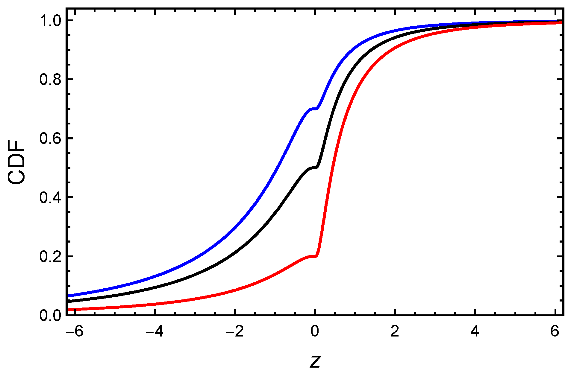
Figure 2 shows the CDF of the DLN distribution for selected parameter values. We can observe that $F_Z\left(0\right)=\overline{\beta }$ and hence $F_Z\left(0\right)$ decreases as $\beta$ increases.

Figure 2. CDF of the DLN distribution: $\left(\beta , {\mu }_1, {\sigma }_1, {\mu }_2, {\sigma }_2\right)$: (0.3, −0.5, 1, 0.5, 1) (), (0.5, −0.5, 1, 0.5, 1) (), $(0.8, -0.5, 1, 0.5, 1)$ ().

2.3. Hazard Rate Function

The survival function of the DLN distribution is

$$\begin{array}{c}\hfill {\displaystyle S_Z\left(z\right)=P(Z>z)=\left\{\begin{array}{cc}{\displaystyle 1-\overline{\beta }{S}_{X_2}\left(\left|z\right|;{\mu }_2,{\sigma }_2\right),}\hfill & z<0,\hfill \\ {\displaystyle \beta S_{X_1}\left(z;{\mu }_1,{\sigma }_1\right),}\hfill & z\ge 0,\hfill \end{array}\right.}\end{array}$$

(4)

where

$$\begin{array}{c}\hfill {\displaystyle S_{X_j}\left(x;{\mu }_j,{\sigma }_j\right)=P\left(X_j>x\right)=1-\Phi \left(\frac{ln\left(x\right)-{\mu }_j}{{\sigma }_j}\right),x>0,j=1,2}\end{array}$$

are the SFs of the LN distributions.

The hazard rate function (HRF) of the DLN distribution is

$$\begin{array}{c}\hfill {\displaystyle h_Z\left(z\right)=\frac{f_Z\left(z\right)}{S_Z\left(z\right)}=\left\{\begin{array}{cc}{\displaystyle \frac{\overline{\beta }{f}_{X_2}\left(\left|z\right|;{\mu }_2,{\sigma }_2\right)}{1-\overline{\beta }{S}_{X_2}\left(\left|z\right|;{\mu }_2,{\sigma }_2\right)},}\hfill & z<0,\hfill \\ {\displaystyle \frac{f_{X_1}\left(z\right)}{S_{X_1}\left(z;{\mu }_1,{\sigma }_1\right)},}\hfill & z\ge 0.\hfill \end{array}\right.}\end{array}$$

(5)

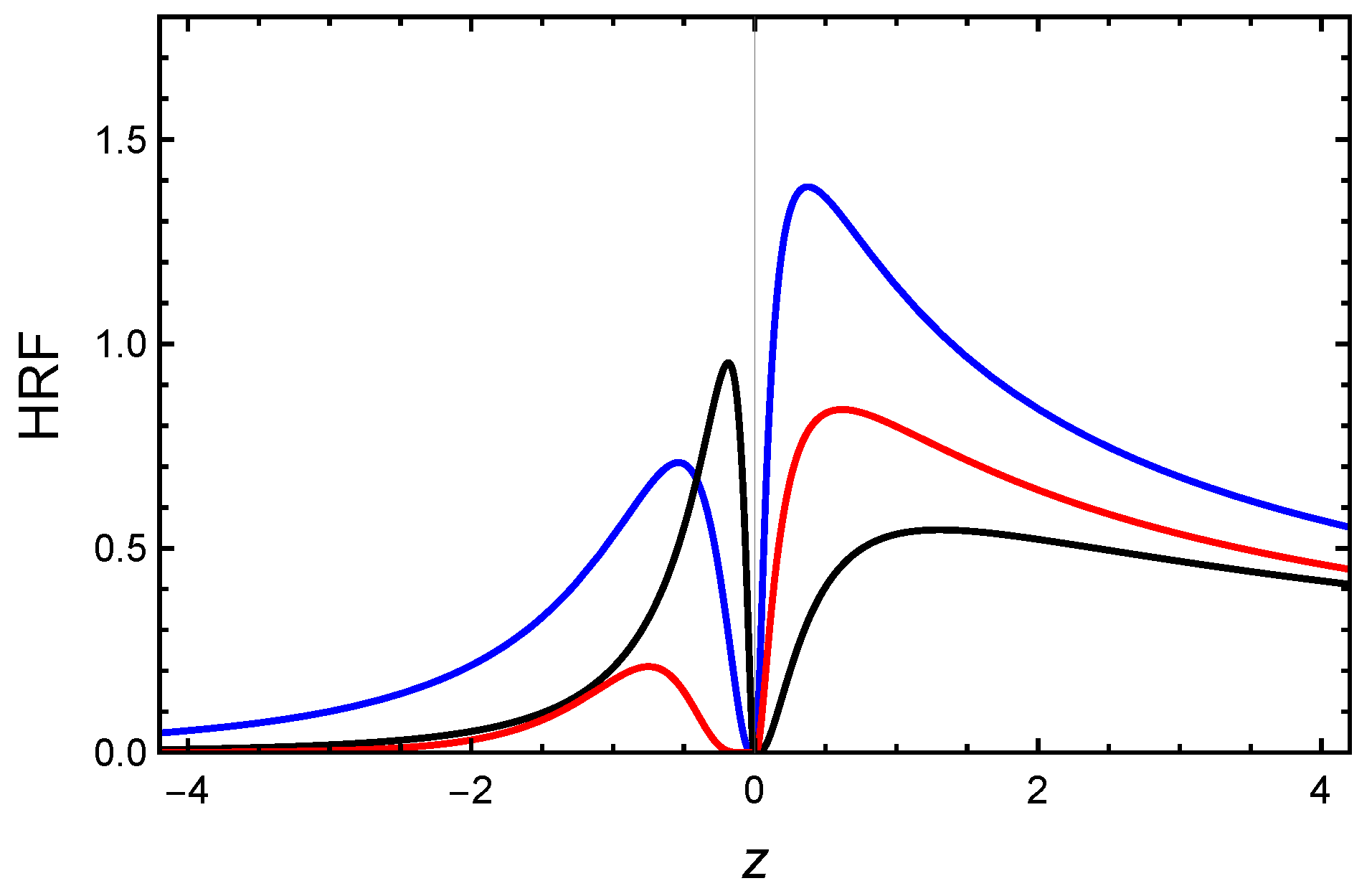
Figure 3 shows the HRF of the DLN distribution for selected parameter values. This figure shows that the HRF of the DLN distribution can be bimodal with one mode on each side of the origin.

Figure 3. HRF of the DLN distribution: $\left(\beta , {\mu }_1, {\sigma }_1, {\mu }_2, {\sigma }_2\right)$: (0.3, −0.5, 1, 0.5, 0.9) (), (0.5, 0.5, 0.9, −0.5, 1) (), $(0.8, 0, 1, 0, 0.5)$ ().

2.4. Moments and Associated Measures

The rth raw moment of the DLN distribution is

$$\begin{array}{c}\hfill {\displaystyle E\left(Z^r\right)=\beta E\left(X_1^r\right)+{(-1)}^r\overline{\beta }E\left(X_2^r\right),r\ge 1,}\end{array}$$

(6)

where

$$\begin{array}{c}\hfill {\displaystyle E\left(X_j^r\right)=e^{r{\mu }_j+r^2{\sigma }_j^2/2},j=1,2}\end{array}$$

(7)

are the rth moments of the LN distributions.

In particular, the first four raw moments of Z are

$$\begin{array}{ccc}\hfill {\displaystyle E\left(Z\right)}& =& \beta e^{{\mu }_1+{\sigma }_1^2/2}-\overline{\beta }{e}^{{\mu }_2+{\sigma }_2^2/2},\hfill \\ \hfill {\displaystyle E\left(Z^2\right)}& =& \beta e^{2{\mu }_1+2{\sigma }_1^2}+\overline{\beta }{e}^{2{\mu }_2+2{\sigma }_2^2},\hfill \\ \hfill {\displaystyle E\left(Z^3\right)}& =& \beta e^{3{\mu }_1+9{\sigma }_1^2/2}-\overline{\beta }{e}^{3{\mu }_2+9{\sigma }_2^2/2},\hfill \\ \hfill {\displaystyle E\left(Z^4\right)}& =& \beta e^{4{\mu }_1+8{\sigma }_1^2}+\overline{\beta }{e}^{4{\mu }_2+8{\sigma }_2^2}.\hfill \end{array}$$

The variance, skewness and kurtosis of the DLN distribution can be obtained using the well-known expressions:

$$\begin{array}{ccc}\hfill {\displaystyle Variance\left(Z\right)}& =& E\left(Z^2\right)-{\left[E\left(Z\right)\right]}^2,\hfill \\ \hfill {\displaystyle Skewness\left(Z\right)}& =& \frac{E\left(Z^3\right)-3E\left(Z^2\right)E\left(Z\right)+2{\left[E\left(Z\right)\right]}^3}{{\left[Var\left(Z\right)\right]}^{3/2}},\hfill \\ \hfill {\displaystyle Kurtosis\left(Z\right)}& =& \frac{E\left(Z^4\right)-4E\left(Z^3\right)E\left(Z\right)+6E\left(Z^2\right){\left[E\left(Z\right)\right]}^2-3{\left[E\left(Z\right)\right]}^3}{{\left[Var\left(Z\right)\right]}^2}\hfill \end{array}$$

upon substituting for the raw moments.

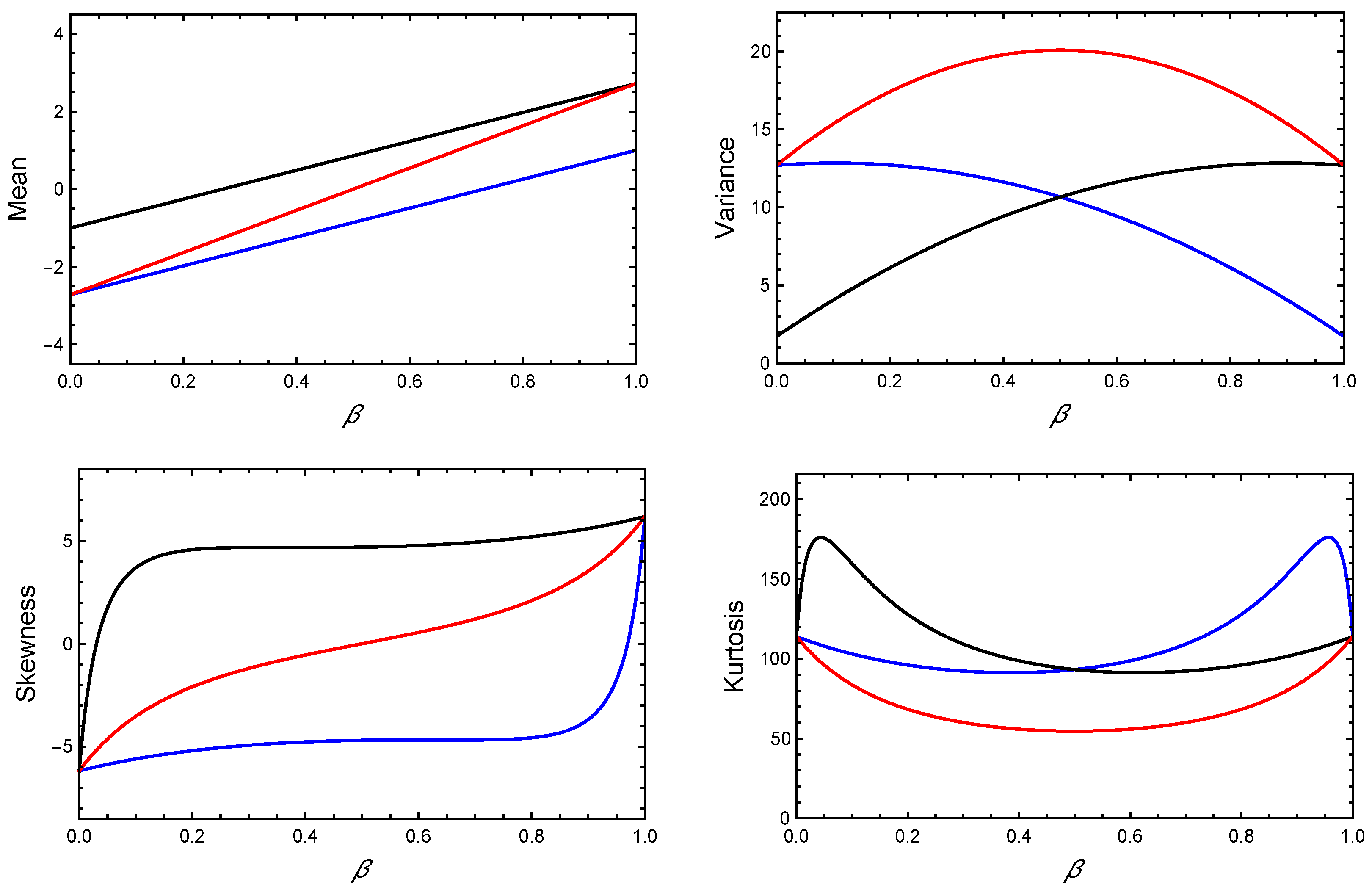
Figure 4 shows the mean, variance, skewness and kurtosis of the DLN distribution as a function of $\beta$ for selected values of $\left({\mu }_1,{\sigma }_1,{\mu }_2,{\sigma }_2\right)$. We can observe that the skewness can be negative or positive, i.e., the DLN distribution can be skewed to the left or skewed to the right.

Figure 4. Mean, variance, skewness and kurtosis of the DLN distribution as a function of $\beta$: $\left({\mu }_1, {\sigma }_1, {\mu }_2, {\sigma }_2\right):(-0.5, 1, 0.5,1)$ (), $(0.5, 1, -0.5, 1)$ (), $(0.5, 1, 0.5, 1)$ ().

2.5. Harmonic Mean

The harmonic mean of an RV V is defined as

$$\begin{array}{c}\hfill {\displaystyle HM\left(V\right)=\frac{1}{E[1/V]},}\end{array}$$

provided $E[1/V]$ exists.

Proposition 1.

The harmonic mean of the RSMT Z is

$$\begin{array}{c}\hfill {\displaystyle HM\left(Z\right)=\frac{1}{\frac{\beta }{HM\left(X_1\right)}-\frac{\overline{\beta }}{HM\left(X_2\right)}}.}\end{array}$$

Proof. 

Since

$$\begin{array}{ccc}\hfill {\displaystyle \frac{1}{HM\left(Z\right)}}& =& {\displaystyle E[1/Z]}\hfill \\ & =& {\displaystyle {\int }_0^{\infty }\frac{1}{z}\beta f_{X_1}\left(z\right)dz+{\int }_{-\infty }^0\frac{1}{z}\overline{\beta }{f}_{X_2}(-z)dz}\hfill \\ & =& {\displaystyle \beta E\left[1/X_1\right]-\overline{\beta }E\left[1/X_2\right]}\hfill \\ & =& {\displaystyle \frac{\beta }{HM\left(X_1\right)}-\frac{\overline{\beta }}{HM\left(X_2\right)},}\hfill \end{array}$$

the proposition follows. □

Corollary 1.

The harmonic mean of the DLN distribution is

$$\begin{array}{c}\hfill {\displaystyle HM\left(Z\right)=\frac{1}{\frac{\beta }{HM\left(X_1\right)}-\frac{\overline{\beta }}{HM\left(X_2\right)}},}\end{array}$$

where

$$\begin{array}{c}\hfill {\displaystyle HM\left(X_j\right)=e^{{\mu }_j-{\sigma }_j^2/2},j=1,2}\end{array}$$

are the harmonic means of the LN distributions.

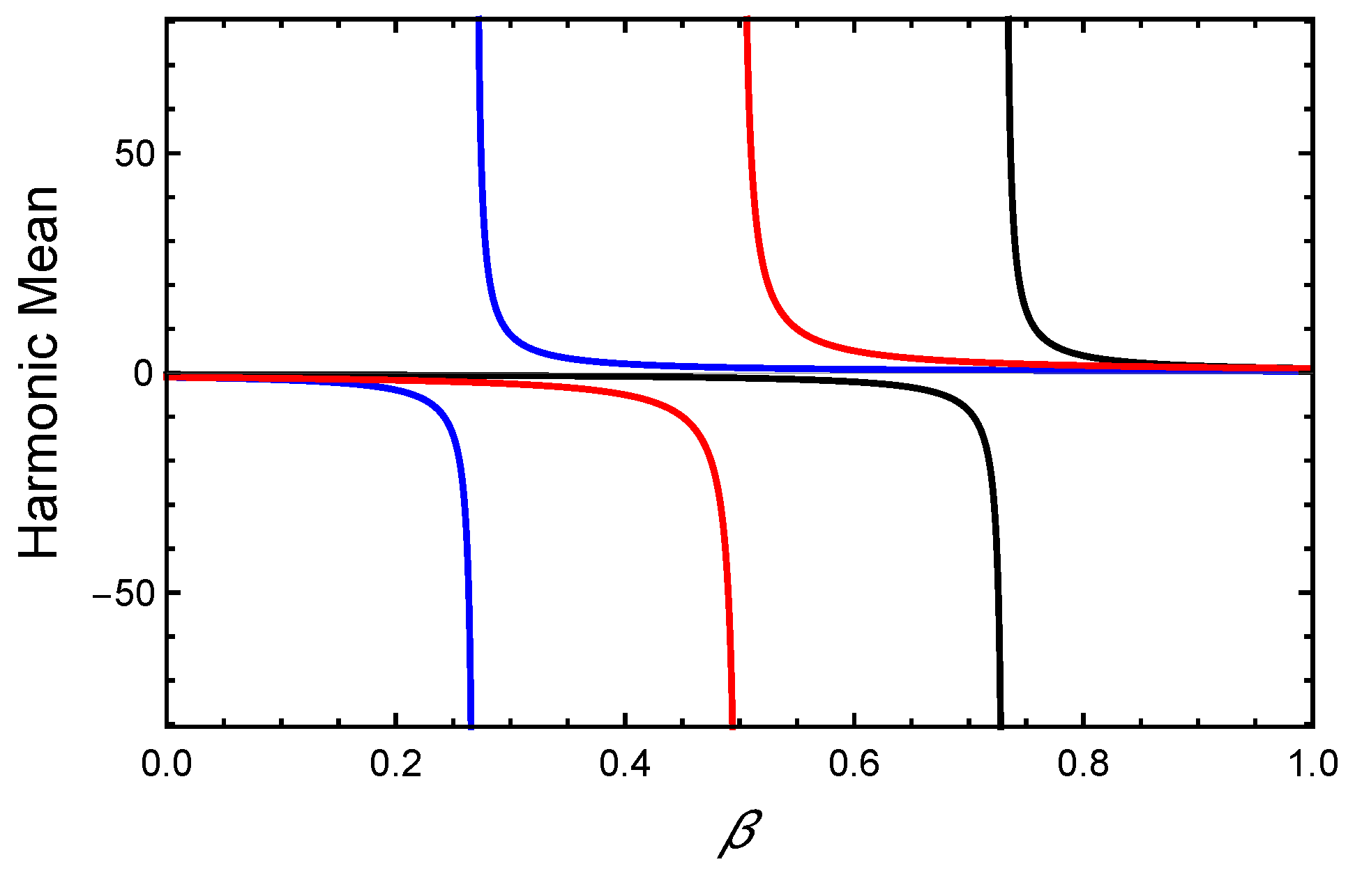
Figure 5 shows the harmonic mean of the DLN distribution as a function of $\beta$ for selected parameter values.

Figure 5. Harmonic mean of the DLN distribution as a function of $\beta$: $\left({\mu }_1, {\sigma }_1, {\mu }_2, {\sigma }_2\right)$: (−0.5, 1, 0.5, 1) (), $(0.5, 1, -0.5, 1)$ (), $(0.5, 1, 0.5, 1)$ ().

2.6. Entropies

Entropies are measures of a system’s variation, instability or unpredictability. For an RV V with PDF $f_V\left(v\right)$, the following are two well-known entropies:

1.

Tsallis entropy [17]:

$$\begin{array}{c}\hfill {\displaystyle T_{\alpha }\left(V\right)=\frac{1}{\alpha -1}\left\{1-E\left[f_V^{\alpha -1}\left(V\right)\right]\right\},0<\alpha \ne 1.}\end{array}$$

2.

Shannon entropy [18]:

$$\begin{array}{c}\hfill {\displaystyle H\left(V\right)=-E\left[ln{f}_V\left(V\right)\right]=\underset{\alpha \to 1}{lim}{T}_{\alpha }\left(V\right).}\end{array}$$

Proposition 2.

The Tsallis entropy of the RSMT Z is

$$\begin{array}{c}\hfill {\displaystyle T_{\alpha }\left(Z\right)=T_{\alpha }\left(Y\right)+{\beta }^{\alpha }{T}_{\alpha }\left(X_1\right)+{\overline{\beta }}^{\alpha }{T}_{\alpha }\left(X_2\right)}\end{array}$$

for $0<\alpha \ne 1$, where

$$\begin{array}{c}\hfill {\displaystyle T_{\alpha }\left(Y\right)=\frac{1-{\beta }^{\alpha }-{\overline{\beta }}^{\alpha }}{\alpha -1}.}\end{array}$$

Proof. 

See [16]. □

Corollary 2.

The Shannon entropy of the RSMT Z is

$$\begin{array}{c}\hfill {\displaystyle H\left(Z\right)=\underset{\alpha \to 1}{lim}{T}_{\alpha }\left(Z\right)=H\left(Y\right)+\beta H\left(X_1\right)+\overline{\beta }H\left(X_2\right),}\end{array}$$

where

$$\begin{array}{c}\hfill {\displaystyle H\left(Y\right)=\underset{\alpha \to 1}{lim}{T}_{\alpha }\left(Y\right)=-\beta ln\left(\beta \right)-\overline{\beta }ln\left(\overline{\beta }\right).}\end{array}$$

Proposition 3.

The Tsallis entropy of the LN distribution with parameters $(\mu ,\sigma )$ is

$$\begin{array}{c}\hfill {\displaystyle T_{\alpha }\left(X\right)=\frac{1}{\alpha -1}\left\{1-{\left(\frac{1}{\sqrt{2\pi }\sigma }\right)}^{\alpha -1}\frac{1}{\sqrt{\alpha }}exp\left[\mu (1-\alpha )+\frac{{\sigma }^2}{2\alpha }{(1-\alpha )}^2\right]\right\}}\end{array}$$

for $0<\alpha \ne 1$.

Proof. 

Since

$$\begin{array}{ccc}\hfill {\displaystyle 1-(\alpha -1)T_{\alpha }\left(X\right)}& =& {\displaystyle {\int }_0^{\infty }{f}_X^{\alpha }\left(x\right)dx}\hfill \\ & =& {\displaystyle {\int }_0^{\infty }{\left(\frac{1}{\sqrt{2\pi }\sigma }\right)}^{\alpha }\frac{1}{x^{\alpha }}exp\left\{-\frac{\alpha }{2{\sigma }^2}{\left[ln\left(x\right)-\mu \right]}^2\right\}dx}\hfill \\ & =& {\displaystyle {\left(\frac{1}{\sqrt{2\pi }\sigma }\right)}^{\alpha }{\int }_{-\infty }^{\infty }{e}^{(1-\alpha )y}exp\left[-\frac{1}{2{\left(\sigma /\sqrt{\alpha }\right)}^2}{(y-\mu )}^2\right]dy}\hfill \\ & =& {\displaystyle {\left(\frac{1}{\sqrt{2\pi }\sigma }\right)}^{\alpha -1}\frac{1}{\sqrt{\alpha }}exp\left[\mu (1-\alpha )+\frac{{\sigma }^2}{2\alpha }{(1-\alpha )}^2\right],}\hfill \end{array}$$

the proposition follows. □

Corollary 3.

The Shannon entropy of the LN distribution with parameters $(\mu ,\sigma )$ is

$$\begin{array}{c}\hfill {\displaystyle H\left(X\right)=\underset{\alpha \to 1}{lim}{T}_{\alpha }\left(X\right)=\frac{1}{2}+\mu +ln\left(\sqrt{2\pi }\sigma \right).}\end{array}$$

Proposition 4.

The Tsallis entropy of $Z\sim \mathrm{DLN}\left(\beta , {\mu }_1, {\sigma }_1, {\mu }_2, {\sigma }_2\right)$ is

$$\begin{array}{c}\hfill {\displaystyle T_{\alpha }\left(Z\right)=T_{\alpha }\left(Y\right)+{\beta }^{\alpha }{T}_{\alpha }\left(X_1\right)+{\overline{\beta }}^{\alpha }{T}_{\alpha }\left(X_2\right)}\end{array}$$

for $0<\alpha \ne 1$, where

$$\begin{array}{c}\hfill {\displaystyle T_{\alpha }\left(Y\right)=\frac{1-{\beta }^{\alpha }-{\overline{\beta }}^{\alpha }}{\alpha -1}}\end{array}$$

and

$$\begin{array}{c}\hfill {\displaystyle T_{\alpha }\left(X_j\right)=\frac{1}{\alpha -1}\left\{1-{\left(\frac{1}{\sqrt{2\pi }{\sigma }_j}\right)}^{\alpha -1}\frac{1}{\sqrt{\alpha }}exp\left[{\mu }_j(1-\alpha )+\frac{{\sigma }_j^2}{2\alpha }{(1-\alpha )}^2\right]\right\},j=1,2.}\end{array}$$

The proof of Proposition 4 follows directly from Propositions 2 and 3.

Corollary 4.

The Shannon entropy of $Z\sim \mathrm{DLN}\left(\beta , {\mu }_1, {\sigma }_1, {\mu }_2, {\sigma }_2\right)$ is

$$\begin{array}{c}\hfill {\displaystyle H\left(Z\right)=H\left(Y\right)+\beta H\left(X_1\right)+\overline{\beta }H\left(X_2\right),}\end{array}$$

where

$$\begin{array}{c}\hfill {\displaystyle H\left(Y\right)=-\beta ln\left(\beta \right)-\overline{\beta }ln\left(\overline{\beta }\right)}\end{array}$$

and

$$\begin{array}{c}\hfill {\displaystyle H\left(X_j\right)=\frac{1}{2}+{\mu }_j+ln\left(\sqrt{2\pi }{\sigma }_j\right),j=1,2.}\end{array}$$

Figure 6 shows the Tsallis and Shannon entropies of the DLN distribution as a function of $\beta$ for selected parameter values.

Figure 6. Tsallis and Shannon entropies of the DLN distribution as a function of $\beta$: $\left({\mu }_1, {\sigma }_1, {\mu }_2, {\sigma }_2\right)$: $(-3, 1, 3, 1)$ (), (3, 1, −3, 1) (), (0, 1, 0, 1) ().

Note that the Tsallis and Shannon entropies can be negative for continuous distributions.

3. Maximum Likelihood Estimation

In this section, MLEs of the parameters of the DLN distribution and their asymptotic distributions are derived.

Let $z_1, z_2,\dots ,z_n$ be a random sample from the DLN$\left(\beta ,{\mu }_1, {\sigma }_1, {\mu }_2, {\sigma }_2\right)$ distribution. The log-likelihood function is

$$\begin{array}{c}\hfill {\displaystyle lnL\left(\beta , {\mu }_1, {\sigma }_1, {\mu }_2, {\sigma }_2\right)={\displaystyle \sum _{i=1}^n}ln\left[\beta f_{X_1}\left(z_i; {\mu }_1, {\sigma }_1\right)\right]{\mathbf{1}}_{\left\{z_i>0\right\}}+{\displaystyle \sum _{i=1}^n}ln\left[\overline{\beta }{f}_{X_2}\left(\left|z_i\right|;{\mu }_2, {\sigma }_2\right)\right]{\mathbf{1}}_{\left\{z_i<0\right\}},}\end{array}$$

where ${\mathbf{1}}_A$ denotes the indicator function. The MLEs of the parameters $\left(\beta , {\mu }_1, {\sigma }_1, {\mu }_2, {\sigma }_2\right)$ are:

$$\begin{array}{ccc}\hfill {\displaystyle \widehat{\beta }}& =& \frac{n_1}{n},\hfill \\ \hfill {\displaystyle {\widehat{\mu }}_1}& =& \frac{1}{n_1}{\displaystyle \sum _{i=1}^n}ln\left(z_i\right){\mathbf{1}}_{\left(z_i>0\right)},\hfill \\ \hfill {\displaystyle {\widehat{\sigma }}_1}& =& \sqrt{\frac{1}{n_1}\sum _{i=1}^n{\left[ln\left(z_i\right)-{\widehat{\mu }}_1\right]}^2{\mathbf{1}}_{\left(z_i>0\right)}},\hfill \\ \hfill {\displaystyle {\widehat{\mu }}_2}& =& \frac{1}{n_2}{\displaystyle \sum _{i=1}^n}ln\left(\left|z_i\right|\right)1_{\left(z_i<0\right)},\hfill \\ \hfill {\displaystyle {\widehat{\sigma }}_2}& =& \sqrt{\frac{1}{n_2}\sum _{i=1}^n{\left[ln\left(\left|z_i\right|\right)-{\widehat{\mu }}_2\right]}^2{\mathbf{1}}_{\left(z_i<0\right)}},\hfill \end{array}$$

where

$$\begin{array}{c}\hfill {\displaystyle n_1={\displaystyle \sum _{i=1}^n}{1}_{\left(z_i>0\right)},n_2={\displaystyle \sum _{i=1}^n}{1}_{\left(z_i<0\right)},n_1+n_2=n.}\end{array}$$

The Fisher information matrix about $\left(\beta , {\mu }_1, {\sigma }_1, {\mu }_2, {\sigma }_2\right)$ is

$$\begin{array}{c}\hfill {\displaystyle \mathbf{I}\left(\beta ,{\mu }_1,{\sigma }_1,{\mu }_2,{\sigma }_2\right)=\left[\begin{array}{ccc}{\displaystyle I_Y\left(\beta \right)}& \mathbf{0}& \mathbf{0}\\ {\displaystyle \mathbf{0}}& \beta {\mathbf{I}}_{X_1}\left({\mu }_1,{\sigma }_1\right)& \mathbf{0}\\ \mathbf{0}& \mathbf{0}& \overline{\beta }{\mathbf{I}}_{X_2}\left({\mu }_2,{\sigma }_2\right)\end{array}\right]}\end{array}$$

, where $I_Y\left(\beta \right)=\frac{1}{\beta \overline{\beta }}$ is the Fisher information matrix about $\beta$ and ${\mathbf{I}}_{X_j}\left({\mu }_j,{\sigma }_j\right)=\mathrm{diag}(\frac{1}{{\sigma }_j^2},\frac{2}{{\sigma }_j^2}),j=1,2$ is the Fisher information matrix about $\left({\mu }_j,{\sigma }_j\right)$.

Moreover, the asymptotic distribution of the MLEs as $n\to \infty$ is

$$\begin{array}{c}\hfill {\displaystyle \sqrt{n}\left[\begin{array}{c}{\displaystyle \widehat{\beta }-\beta }\\ {\displaystyle {\widehat{\mu }}_1-{\mu }_1}\\ {\displaystyle {\widehat{\sigma }}_1-{\sigma }_1}\\ {\displaystyle {\widehat{\mu }}_2-{\mu }_2}\\ {\displaystyle {\widehat{\sigma }}_2-{\sigma }_2}\end{array}\right]\stackrel{d}{⟶}MVN\left(\mathbf{0},{\mathbf{I}}^{-1}\left(\beta ,{\mu }_1,{\sigma }_1,{\mu }_2,{\sigma }_2\right)\right),}\end{array}$$

where $\stackrel{d}{⟶}$ denotes convergence in distribution, $MVN$ stands for multivariate normal distribution and

$$\begin{array}{c}\hfill {\displaystyle {\mathbf{I}}^{-1}\left(\beta ,{\mu }_1,{\sigma }_1,{\mu }_2,{\sigma }_2\right)=\mathrm{diag}\left(\beta \overline{\beta },\frac{{\sigma }_1^2}{\beta },\frac{{\sigma }_1^2}{2\beta },\frac{{\sigma }_2^2}{\overline{\beta }},\frac{{\sigma }_2^2}{2\overline{\beta }}\right).}\end{array}$$

4. Simulations

This section details simulations to check the finite sample performance of the MLEs of the parameters of the DLN distribution. The performance is evaluated in terms of biases, mean squared errors of the MLEs and coverage probabilities of the corresponding 95% confidence intervals.

The simulation was repeated $M=$ 10,000 times. In each of the M repetitions, a random sample of size $n=50,100,\dots ,500$ was drawn from the DLN distribution with selected parameter values $\left(\beta ,{\mu }_1,{\sigma }_1,{\mu }_2,{\sigma }_2\right)$ = $(0.3,-2,1,-1,2)$, $(0.5,0,1,1,2)$, $(0.8,2,1,-1,2)$ and $(0.547,-2.812,1.016,-2.224,0.764)$, using the following algorithm:

• Generate $Y_i\sim Bernoulli\left(\beta \right),i=1,2,\dots ,n;$
• Generate $X_{1,i}\sim \mathrm{LN}\left({\mu }_1,{\lambda }_1\right),i=1,2,\dots ,n;$
• Generate $X_{2,i}\sim \mathrm{LN}\left({\mu }_2,{\lambda }_2\right),i=1,2,\dots ,n;$
• Set $Z_i=Y_i{X}_{1,i}-\left(1-Y_i\right)X_{2,i},i=1,2,\dots ,n.$

The parameter values $\left(\beta ,{\mu }_1,{\sigma }_1,{\mu }_2,{\sigma }_2\right)=(0.547,-2.812,1.016,-2.224,0.764)$ are those estimated in the real data application in Section 5.

The measures examined in this simulation study are:

• The bias of the MLEs:

  $$\begin{array}{c}\hfill {\displaystyle Bias\left(\widehat{\theta }\right)=\frac{1}{M}{\displaystyle \sum _{j=1}^M}\left({\widehat{\theta }}_j-\theta \right),\theta =\beta ,{\mu }_1,{\sigma }_1,{\mu }_2,{\sigma }_2.}\end{array}$$
• The mean squared error (MSE) of the MLEs:

  $$\begin{array}{c}\hfill {\displaystyle MSE\left(\widehat{\theta }\right)=\frac{1}{M}{\displaystyle \sum _{j=1}^M}{\left({\widehat{\theta }}_j-\theta \right)}^2,\theta =\beta ,{\mu }_1,{\sigma }_1,{\mu }_2,{\sigma }_2.}\end{array}$$
• The coverage probability (CP) of the 95% confidence interval of each parameter:

  $$\begin{array}{c}\hfill {\displaystyle CP\left(\theta \right)=\frac{1}{M}{\displaystyle \sum _{j=1}^M}{\mathbf{1}}_{\left\{\left({\widehat{\theta }}_j-1.96S.E.\left({\widehat{\theta }}_j\right),{\widehat{\theta }}_j+1.96S.E.\left({\widehat{\theta }}_j\right)\right)\right\}},\theta =\beta ,{\mu }_1,{\sigma }_1,{\mu }_2,{\sigma }_2.}\end{array}$$

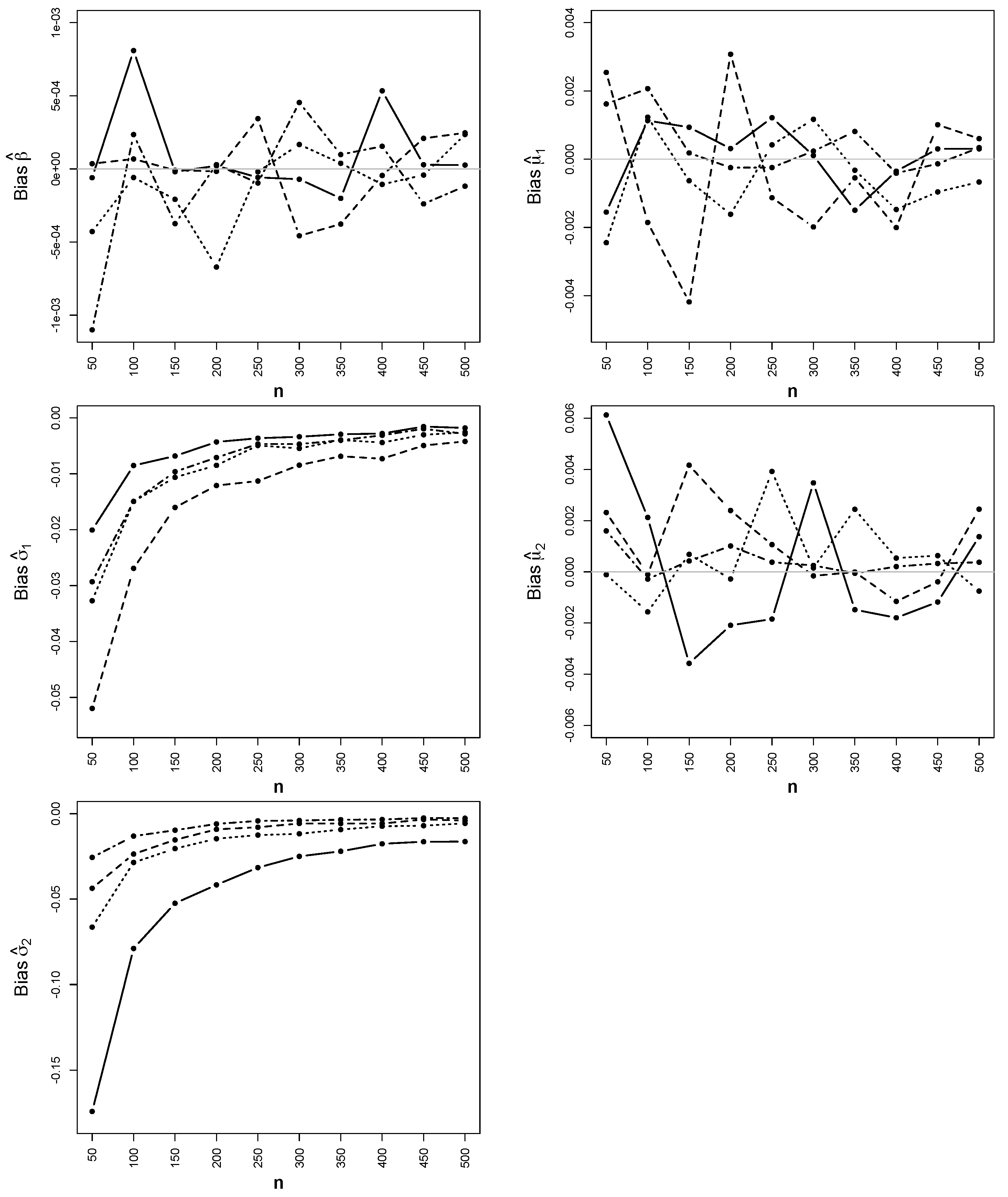
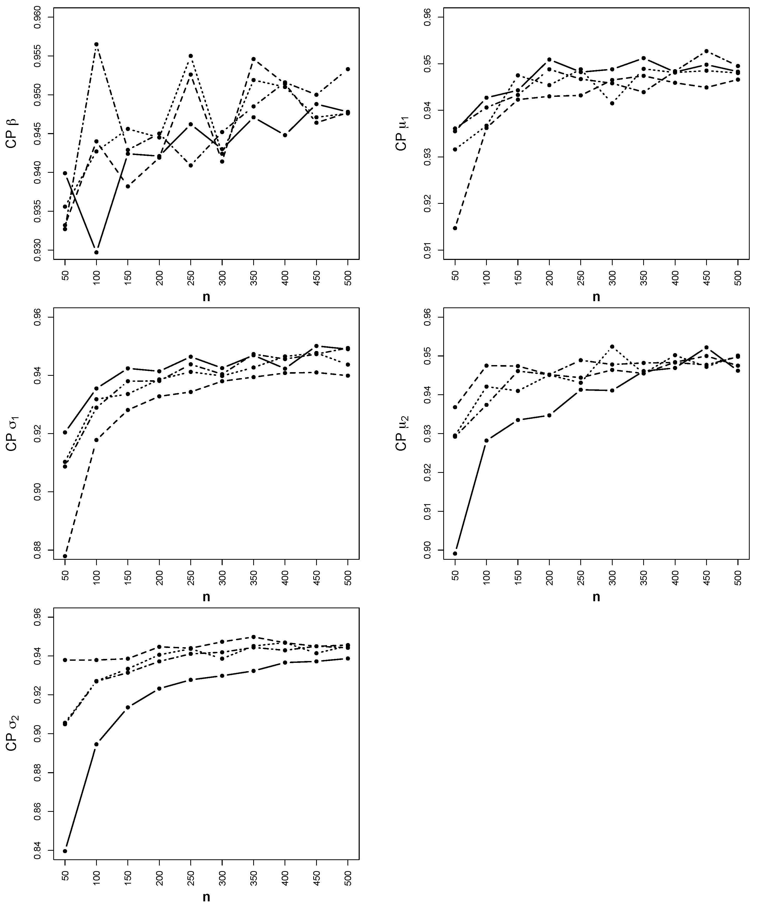
The results of the simulation study are reported in Figure 7, Figure 8 and Figure 9.

• Figure 7 shows that the absolute biases of the MLEs are small and approach zero as n increases.
• Figure 8 shows that the MSEs of the MLEs are small and decrease as n increases.
• Figure 9 shows that the coverage probabilities of the 95% confidence intervals are close to the nominal level.

Figure 7. Bias of the MLEs of the parameters of the DLN distribution: $\left(\beta ,{\mu }_1,{\sigma }_1,{\mu }_2,{\sigma }_2\right)$: $(0.3,-2,1,-1,2)$ (), (0.5, 0, 1, 1, 2) ( - - -), $(0.8,2,1,-1,2)$$\left(.....\right)$, $(0.547,-2.812,1.016,-2.224,0.764)\left(-.-\right)$.

Figure 8. MSE of the MLEs of the parameters of the DLN distribution: $\left(\beta ,{\mu }_1,{\sigma }_1,{\mu }_2,{\sigma }_2\right)$: $(0.3,-2,1,-1,2)$ (), (0.5, 0, 1, 1, 2) ( - - -), $(0.8,2,1,-1,2)$ ($.....$), (0.547, −2.812, 1.016, −2.224, 0.764) ($-.-$).

Figure 9. CP of the 95% confidence intervals of the parameters of the DLN distribution: $\left(\beta ,{\mu }_1,{\sigma }_1,{\mu }_2,{\sigma }_2\right)$: (0.3, −2, 1, −1, 2) (), (0.5, 0, 1, 1, 2) (- - -), (0.8, 2, 1, −1, 2) ($.....$), (0.547, −2.812, 1.016, −2.224, 0.764) ($-.-$).

These conclusions show that the MLEs of the DLN distribution are well behaved for point as well as interval estimation.

5. Application

In this section, we apply the proposed DLN distribution to a real data set from a DNA microarray reported in [19]. According to Wikipedia, “A DNA microarray (also commonly known as DNA chip or biochip) is a collection of microscopic DNA spots attached to a solid surface. Scientists use DNA microarrays to measure the expression levels of large numbers of genes simultaneously or to genotype multiple regions of a genome”. The data labelled as “SID 377353, ESTs [5’:, 3’:AA055048]” consist of the following 118 observations: 0.029, 0.062, 0.011, 0.009, 0.065, −0.128, 0.133, 0.116, 0.184, 0.111, −0.066, −0.049, 0.05, 0.137, 0.162, 0.173, 0.033, 0.107, 0.11, 0.147, 0.118, 0.172, 0.284, −0.137, 0.038, −0.145, −0.181, −0.155, 0.198, 0.024, 0.079, −0.252, 0.062, 0.097, 0.032, 0.026, 0.195, 0.019, 0.138, −0.3, −0.105, −0.11, −0.168, −0.173, −0.15, 0.078, 0.113, −0.047, 0.024, 0.001, −0.075, 0.014, 0.058, −0.083, −0.339, −0.177, −0.073, −0.044, −0.106, −0.159, −0.101, −0.074, −0.126, −0.131, −0.22, −0.184, −0.105, 0.173, 0.151, 0.064, −0.007, −0.005, −0.189, −0.219, −0.301, −0.212, −0.088, 0.157, 0.042, 0.184, 0.114, 0.102, 0.119, −0.064, −0.075, 0.073, 0.038, 0.017, −0.134, −0.118, −0.097, 0.059, 0.025, −0.102, −0.096, −0.035, 0.057, −0.055, 0.015, −0.23, −0.115, 0.255, 0.034, 0.078, 0.129, 0.081, 0.032, 0.047, −0.145, 0.012, −0.224, 0.074, −0.06, −0.137, 0.034, 0.009, −0.139, −0.141.

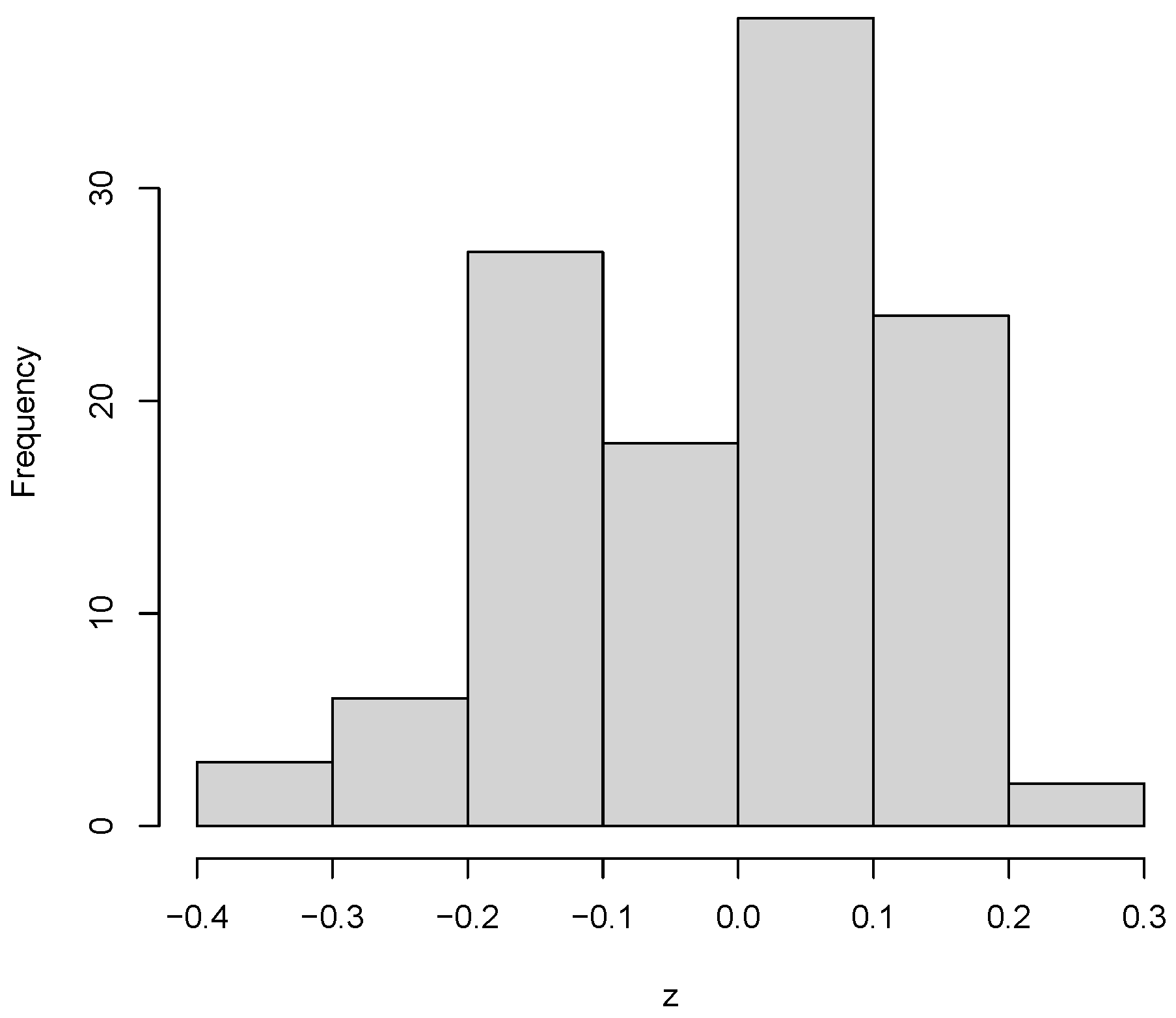
Figure 10 shows the histogram of the data, which indicates bimodality around the origin.

Figure 10. Histogram of the microarray data.

For the sake of comparing the bimodal DLN distribution with other bimodal distributions, we consider the double inverse Gaussian (DIG) distribution proposed in [16]. The PDF of the DIG distribution is

$$\begin{array}{c}\hfill {\displaystyle f_Z\left(z\right)=\left\{\begin{array}{cc}{\displaystyle \overline{\beta }{f}_{X_2}\left(\left|z\right|;{\nu }_2,{\lambda }_2\right),}\hfill & z<0,\hfill \\ {\displaystyle \beta f_{X_1}\left(z;{\nu }_1,{\lambda }_1\right),}\hfill & z\ge 0,\hfill \end{array}\right.}\end{array}$$

(8)

where

$$\begin{array}{c}\hfill {\displaystyle f_{X_j}\left(x;{\nu }_j,{\lambda }_j\right)=\sqrt{\frac{{\lambda }_j}{2\pi }}{x}^{-3/2}exp\left[-\frac{{\lambda }_j{\left(x-{\nu }_j\right)}^2}{2{\nu }_j^{2}x}\right],x>0,{\nu }_j,{\lambda }_j>0,j=1,2}\end{array}$$

(9)

are the PDFs of inverse Gaussian distributions.

Table 1 gives the MLEs, their standard errors (S.E.s), estimated log-likelihoods and Kolmogrov–Smirnov (KS), Anderson–Darling (AD) and Cramér–von Mises (CVM) goodness-of-fit tests of the fitted DIG and DLN distributions. This table shows that the MLE of $\beta$ and its S.E. are the same for both the fitted DIG and DLN distributions, since the Bernoulli parameter $\beta$ is estimated independently in the RSMT. In addition, this table shows that the MLEs of ${\mu }_1$ and ${\mu }_2$ in the fitted DLN distribution are both negative.

Table 1. Summary of the fitted DIG and DLN distributions for DNA microarray data.

Model	Parameter	MLE	S.E.	$ln\widehat{\mathit{L}}$	KS (p-Value)	AD (p-Value)	CVM (p-Value)
DIG	$\beta$	0.542	0.046	39.249	0.126 (0.046)	3.285 (0.020)	0.545 (0.030)
	${\nu }_1$	0.087	0.017
	${\lambda }_1$	0.036	0.006
	${\nu }_2$	0.132	0.018
	${\lambda }_2$	0.126	0.024
DLN	$\beta$	0.542	0.046	64.829	0.065 (0.709)	0.851 (0.446)	0.103 (0.570)
	${\mu }_1$	−2.812	0.127
	${\sigma }_1$	1.016	0.090
	${\mu }_2$	−2.224	0.104
	${\sigma }_2$	0.764	0.074

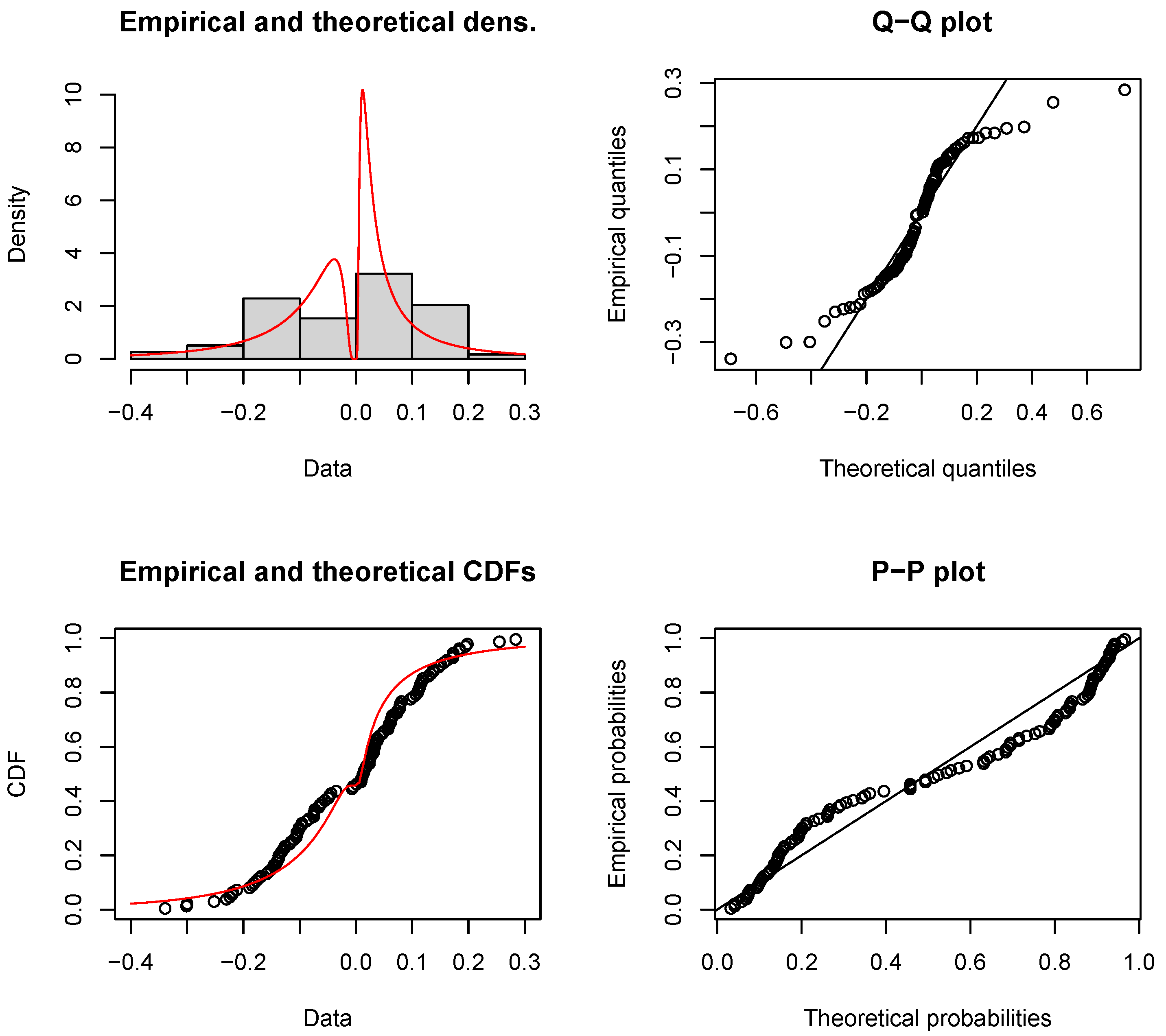
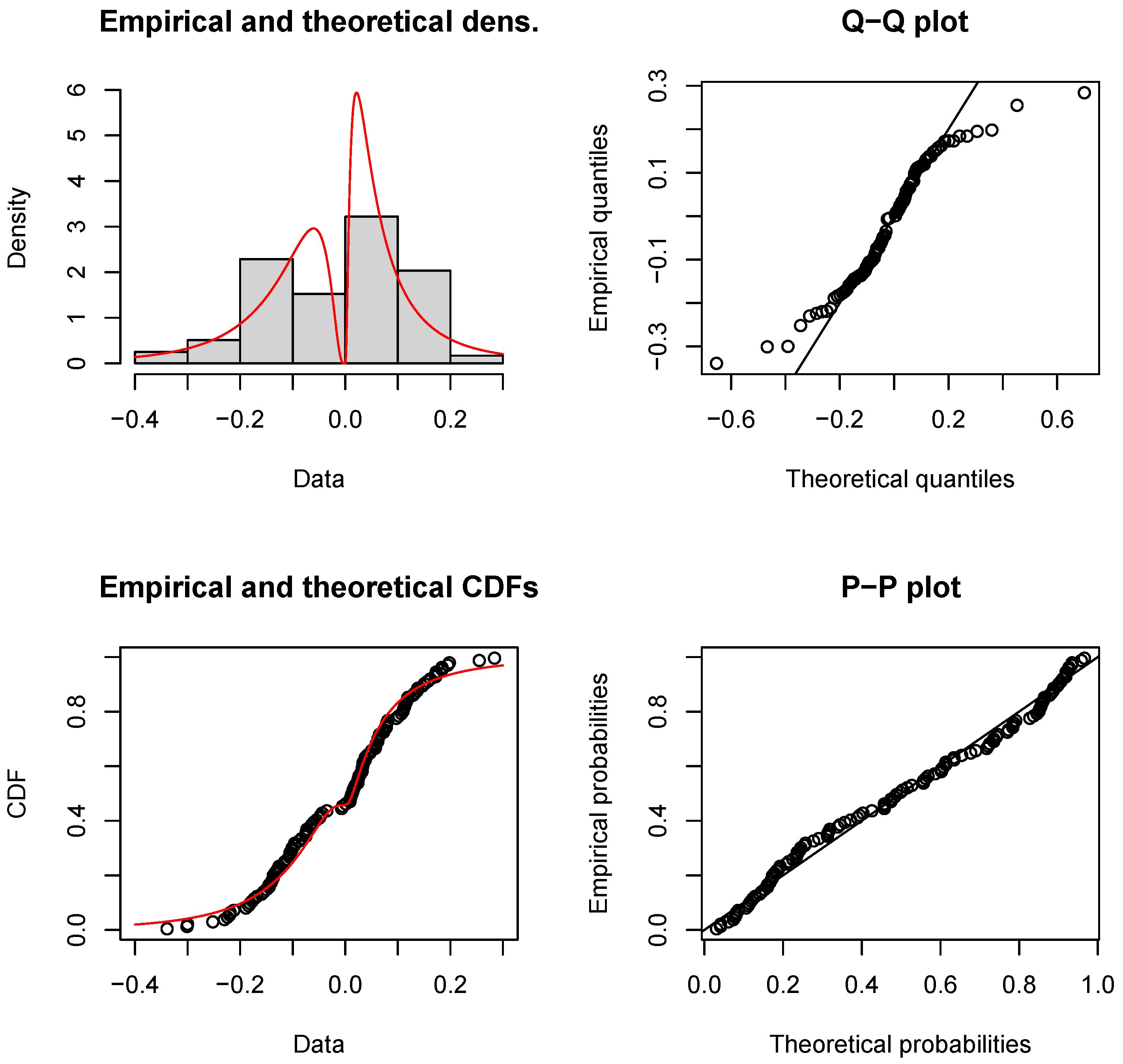
Table 1 shows that the three goodness-of-fit tests have much smaller (larger) test statistics for the fitted DLN (DIG) distribution. This table also shows that the three goodness-of-fit tests reject (accept) the DIG (DLN) distribution for the given data. This conclusion is supported by the diagnostic plots in Figure 11 and Figure 12. In these figures, (i) the PDF and CDF plots indicate, in an informal way, that the fitted DIG (DLN) distribution may not be suitable for the given data; (ii) the quantile–quantile (Q–Q) plots show that the fitted DIG and DLN distributions inappropriately describe the tails of the distributions; (iii) the probability–probability (P–P) plots show that the fitted DIG (DLN) distribution inappropriately (appropriately) describes the center of the distribution.

Figure 11. Diagnostic plots of the fitted DIG distribution.

Figure 12. Diagnostic plots of the fitted DLN distribution.

6. Conclusions and Comments

We have proposed a bimodal distribution on the real line, referred to as the double log-normal distribution. We have derived its statistical properties, including the probability density, cumulative distribution and hazard rate functions, the moments and associated measures and harmonic mean, as well as Tsallis and Shannon entropies. Additionally, maximum likelihood estimates of the parameters and their asymptotic distribution are provided. Simulation studies showed that the maximum likelihood estimation performed well in terms of the bias, mean squared error and coverage probability of confidence intervals. Application to a DNA microarray data set showed that the proposed distribution is flexible and competitive for modeling bimodal data around the origin.

Instead of the log-normal distribution, one can consider the length biased log-normal distribution developed in [20]. It will be interesting to formulate a double length biased log-normal distribution.

References

1. Crow, E.L.; Shimizu, K. Lognormal Distributions: Theory and Applications; Statistics Textbooks and Monographs; Routledge: London, UK, 2018. [Google Scholar]
2. Aly, E. A unified approach for developing Laplace-type distributions. J. Indian Soc. Probab. Stat. 2018, 19, 245–269. [Google Scholar] [CrossRef]
3. Laplace, P.S. Memoire sur la probabilite des causes par les evenements. Mem. L’Acad. R. Sci. Present. Divers. Savan 1774, 6, 621–656. [Google Scholar]
4. Plucinska, A. On a general form of the probability density function and its application to the investigation of the distribution of rheostat resistence. Zastosow. Mat. 1966, 9, 9–19. [Google Scholar]
5. Balakrishnan, N.; Kocherlakota, S. On the double Weibull distribution: Order statistics and estimation. Sankhya Indian J. Stat. Ser. B 1985, 47, 161–178. [Google Scholar]
6. Kantam, R.R.L.; Narasimham, V.L. Linear estimation in reflected gamma distribution. Sankhya Indian J. Stat. Ser. B 1991, 53, 25–47. [Google Scholar]
7. Nadarajah, S.; Afuecheta, E.; Chan, S. A double generalized Pareto distribution. Stat. Probab. Lett. 2013, 83, 2656–2663. [Google Scholar] [CrossRef]
8. Bindu, P.; Sangita, K. Double Lomax distribution and its applications. Statistica 2015, 75, 331–342. [Google Scholar]
9. Kumar, S.C.; Jose, R. On double Lindley distribution and some of its properties. Am. J. Math. Manag. Sci. 2019, 38, 23–43. [Google Scholar]
10. John, S. The three-parameter two-piece normal family of distributions and its fitting. Commun. Stat. Theory Methods 1982, 11, 879–885. [Google Scholar] [CrossRef]
11. Kimber, A. Methods for the two-piece normal distribution. Commun. Stat. Theory Methods 1985, 14, 235–245. [Google Scholar] [CrossRef]
12. Lingappaiah, G. On two-piece double exponential distribution. J. Korean Stat. Soc. 1988, 17, 46–55. [Google Scholar]
13. Abdulah, E.; Elsalloukh, H. Bimodal Class based on the Inverted Symmetrized Gamma Distribution with Applications. J. Stat. Appl. Probab. 2014, 3, 1–7. [Google Scholar] [CrossRef]
14. Hoseinzadeh, A.; Maleki, M.; Khodadadi, Z.; Contreras-Reyes, J.E. The skew-reflected-Gompertz distribution for analyzing symmetric and asymmetric data. J. Comput. Appl. Math. 2019, 349, 132–141. [Google Scholar] [CrossRef]
15. Halvarsson, D. Maximum likelihood estimation of asymmetric double type II Pareto distributions. J. Stat. Theory Pract. 2020, 14, 22. [Google Scholar] [CrossRef]
16. Almutairi, A.; Ghitany, M.; Alothman, A.; Gupta, R.C. Double Inverse-Gaussian Distributions and Associated Inference. J. Indian Soc. Probab. Stat. 2023, 1–32. [Google Scholar] [CrossRef]
17. Tsallis, C. Possible generalization of Boltzmann-Gibbs statistics. J. Stat. Phys. 1988, 52, 479–487. [Google Scholar] [CrossRef]
18. Shannon, C.E. A Mathematical Theory of Communication. Bell Syst. Tech. J. 1948, 27, 379–423. [Google Scholar] [CrossRef] [Green Version]
19. Cankaya, M. Asymmetric Bimodal Exponential Power Distribution on the Real Line. Entropy 2018, 20, 23. [Google Scholar] [CrossRef] [PubMed] [Green Version]
20. Ratnaparkhi, M.V.; Naik-Nimbalkar, U.V. The Length-biased Lognormal Distribution and its application in the Analysis of data from oil Field Exploration studies. J. Mod. Appl. Stat. Methods 2012, 11, 225–260. [Google Scholar] [CrossRef] [Green Version]
Figure 1. PDF of the DLN distribution: β ,   μ 1 ,   σ 1 ,   μ 2 ,   σ 2 : (0.3, −0.5, 1, 0.5, 1) (Mathematics 11 03360 i001), (0.5, −0.5, 1, 0.5, 1) (Mathematics 11 03360 i002), ( 0.8 ,   0.5 ,   1 ,   0.5 ,   1 ) (Mathematics 11 03360 i003).
Mathematics 11 03360 g001
Figure 2. CDF of the DLN distribution: β ,   μ 1 ,   σ 1 ,   μ 2 ,   σ 2 : (0.3, −0.5, 1, 0.5, 1) (Mathematics 11 03360 i001), (0.5, −0.5, 1, 0.5, 1) (Mathematics 11 03360 i002), ( 0.8 ,   0.5 ,   1 ,   0.5 ,   1 ) (Mathematics 11 03360 i003).
Mathematics 11 03360 g002
Figure 3. HRF of the DLN distribution: β ,   μ 1 ,   σ 1 ,   μ 2 ,   σ 2 : (0.3, −0.5, 1, 0.5, 0.9) (Mathematics 11 03360 i001), (0.5, 0.5, 0.9, −0.5, 1) (Mathematics 11 03360 i002), ( 0.8 ,   0 ,   1 ,   0 ,   0.5 ) (Mathematics 11 03360 i003).
Mathematics 11 03360 g003