On Hermite–Hadamard–Fejér-Type Inequalities for η-Convex Functions via Quantum Calculus

Abstract

In this paper, we use $q_a$- and $q^b$-integrals to establish some quantum Hermite–Hadamard–Fejér-type inequalities for $\eta$-convex functions. By taking $q\to 1$, our results reduce to classical results on Hermite–Hadamard–Fejér-type inequalities for $\eta$-convex functions. Moreover, we give some examples for quantum Hermite–Hadamard–Fejér-type inequalities for $\eta$-convex functions. Some results presented here for $\eta$-convex functions provide extensions of others given in earlier works for convex and $\eta$-convex functions.

1. Introduction

Quantum calculus (sometimes called q-calculus) is known as the study of calculus with no limits. Note that q-calculus can be reduced to ordinary calculus if we stipulate that limit q tends to 1. It was first studied by the famous mathematician Euler (1707–1783). In 1910, F. H. Jackson [1] determined the definite q-integral known as the q-Jackson integral. Quantum calculus has many applications in several mathematical areas such as combinatorics, number theory, orthogonal polynomials, basic hypergeometric functions, mechanics, quantum theory and theory of relativity; see, for instance, refs. [2,3,4,5,6,7] and the references therein. The book by V. Kac and P. Cheung [8] covers the fundamental knowledge and basic theoretical concepts of quantum calculus.

In 2013, J. Tariboon and S. K. Ntouyas [9,10] defined the $q_a$-derivative and $q_a$-integral of a continuous function on finite intervals and proved some of its properties. In 2020, S. Bermudo, P. Korus and J. E. Napoles Valdes [11] defined the $q^b$-derivative and $q^b$-integral of a continuous function on finite intervals. Many well-known integral inequalities such as Hölder, Hermite–Hadamard, trapezoid, Ostrowski, Cauchy–Bunyakovsky–Schwarz, Grüss and Grüss–Čebyšev inequalities have been studied in the concept of q-calculus. Based on these results, there are many outcomes concerning q-calculus.

The Hermite–Hadamard–Fejér integral inequality has been proven in [12] as follows:

Theorem 1 ([12]).

Let $f:[a,b]\to \mathbb{R}$ be a convex function. Then

$$f\left({\displaystyle \frac{a+b}{2}}\right){\int }_a^{b}g\left(x\right)dx\le {\int }_a^{b}f\left(x\right)g\left(x\right)dx\le {\displaystyle \frac{f\left(a\right)+f\left(b\right)}{2}}{\int }_a^{b}g\left(x\right)dx,$$

(1)

where $g:[a,b]\to {\mathbb{R}}^{+}$ is integrable and symmetric about $x={\displaystyle \frac{a+b}{2}}$, i.e., $g\left(x\right)=g(a+b-x)$.

Recently, there have been many works about quantum integral inequalities, especially quantum Hermite–Hadamard–Fejér-type inequalities. Interested readers can see [13,14,15,16,17,18] and the references therein.

Let I be an interval in the real line $\mathbb{R}$. Consider $\eta :A\times A\to B$ for appropriate $A,B\subseteq \mathbb{R}$.

Definition 1.

A function $f:I\to \mathbb{R}$ is called convex with respect to η (η-convex), if

$$f(tx+(1-t\left)y\right)\le f\left(y\right)+t\eta \left(f\right(x),f(y\left)\right)$$

(2)

for all $x,y\in I$ and $t\in [0,1]$.

In fact, the above definition geometrically says that if a function is $\eta$-convex on I, then it is a graph between any $x,y\in I$ and is on or under the path starting from $(y,f(y\left)\right)$ and ending at $(x,f(y)+\eta (f\left(x\right),f\left(y\right)\left)\right)$. If $f\left(x\right)$ should be the endpoint of the path for every $x,y\in I$, then we have $\eta (x,y)=x-y$ and the function reduces to a convex one. Note that by taking $x=y$ in (2), we obtain $t\eta \left(f\right(x),f(x\left)\right)\ge 0$ for any $x\in I$ and $t\in [0,1]$, which implies that $\eta \left(f\right(x),f(x\left)\right)\ge 0$ for any $x\in I$. Also, if we take $t=1$ in (2), we obtain

$$f\left(x\right)-f\left(y\right)\le \eta \left(f\left(x\right),f\left(y\right)\right)$$

for any $x,y\in I.$

There are simple examples about the $\eta$-convexity of a function.

Example 1.

(i) 

Consider a function $f:\mathbb{R}\to \mathbb{R}$ defined as:

$$f\left(x\right)=\left\{\begin{array}{cc}-x,\hfill & \mathit{for}x\ge 0;\hfill \\ x,\hfill & \mathit{for}x<0,\hfill \end{array}\right.$$

and define a bifunction η as $\eta (x,y)=-x-y$, for all $x,y\in {\mathbb{R}}^{-}=\left(-\infty ,0\right].$ It is not hard to check that f is an η-convex function but not a convex one.

(ii) 

Define a function $f:{\mathbb{R}}^{+}\to {\mathbb{R}}^{+}$ as

$$f\left(x\right)=\left\{\begin{array}{cc}x,\hfill & \mathit{for}0\le x\le 1;\hfill \\ 1,\hfill & \mathit{for}x>1,\hfill \end{array}\right.$$

and a bifunction $\eta :{\mathbb{R}}^{+}\times {\mathbb{R}}^{+}\to {\mathbb{R}}^{+}$ as

$$\eta (x,y)=\left\{\begin{array}{cc}x+y,\hfill & \mathit{for}x\le y;\hfill \\ 2(x+y),\hfill & \mathit{for}x>y.\hfill \end{array}\right.$$

Then f is an η-convex function but is not convex.

In 2017, M. R. Delavar and M. De La Sen [19] presented some generalizations of Fejér-type inequalities related to $\eta$-convex functions, which improve the right and left sides of (1), respectively.

This paper generalizes and extends some well-known results for Hermite–Hadamard–Fejér integral inequality for $\eta$-convex functions via quantum integrals. The results presented here would extend some of those in the existing literature.

2. Preliminaries

Now, we recall the following well-known basic concepts of quantum calculus on finite intervals, which are essential in proving our main results.

Let $[a,b]\subseteq \mathbb{R}$ be an interval and $0<q<1$ be a constant. The $q_a$- and $q^b$-derivative of a function $f:[a,b]\to \mathbb{R}$ at a point $x\in [a,b]$ is defined as follows:

Definition 2 ([11]).

Let $f:[a,b]\to \mathbb{R}$ be a continuous function and let $x\in [a,b]$. Then the $q_a$-derivative of f on $[a,b]$ at x is defined as

$${}_a{d}_{q}f\left(x\right)={\displaystyle \frac{f\left(x\right)-f(qx+(1-q\left)a\right)}{(1-q)(x-a)}},x\ne a.$$

(3)

It is obvious that ${\displaystyle {}_a{d}_{q}f\left(a\right)=\underset{x\to a}{lim}{}_a{d}_{q}f\left(x\right).}$

Analogously, the $q^b$-derivative of f on $[a,b]$ at x is defined as

$${}^b{d}_{q}f\left(x\right)={\displaystyle \frac{f\left(x\right)-f(qx+(1-q\left)b\right)}{(1-q)(x-b)}},x\ne b.$$

(4)

It is obvious that ${\displaystyle {}^b{d}_{q}f\left(b\right)=\underset{x\to b}{lim}{}^b{d}_{q}f\left(x\right).}$

A function f is $q_a$- and $q^b$-differentiable on $[a,b]$ if ${}_a{d}_{q}f\left(x\right)$ and ${}^b{d}_{q}f\left(x\right)$ exist for all $x\in [a,b]$. Also, if $a=0$ in (3) or if $b=0$ in (4), then ${}_0{d}_q={}^0{d}_q=D_{q}f$, where $D_q$ is the q-derivative of the function f defined as

$$D_{q}f\left(x\right)={\displaystyle \frac{f\left(x\right)-f\left(qx\right)}{(1-q)x}}.$$

Let us elaborate on the above definitions with the help of examples.

Example 2.

Let $\alpha ,\beta \in \mathbb{R},x\in [a,b]$ and $0<q<1$. Then for $x\ne a$, we have

$$\begin{array}{cc}\hfill {}_a{d}_q(\alpha x^2+\beta )& ={\displaystyle \frac{(\alpha x^2+\beta )-[\alpha {(qx+(1-q)a)}^2+\beta ]}{(1-q)(x-a)}}\hfill \\ \hfill & ={\displaystyle \frac{\alpha x^2(1+q)-2\alpha qax-\alpha a^2(1-q)}{x-a}}\hfill \\ \hfill & =\alpha x(1+q)+\alpha a(1-q).\hfill \end{array}$$

Note that when $x=a$, we have ${\displaystyle \underset{x\to a}{lim}\left({}_a{d}_q(\alpha x^2+\beta )\right)=2\alpha a.}$

Moreover, for $x\ne b$, we have

$$\begin{array}{cc}\hfill {}^b{d}_q(\alpha x^2+\beta )& ={\displaystyle \frac{(\alpha x^2+\beta )-[\alpha {(qx+(1-q)b)}^2+\beta ]}{(1-q)(x-b)}}\hfill \\ \hfill & ={\displaystyle \frac{\alpha x^2(1+q)-2\alpha qbx-\alpha b^2(1-q)}{x-b}}\hfill \\ \hfill & =\alpha x(1+q)+\alpha b(1-q).\hfill \end{array}$$

Note that when $x=b$, we have ${\displaystyle \underset{x\to b}{lim}\left({}^b{d}_q(\alpha x^2+\beta )\right)=2\alpha b.}$

J. Tariboon and S. K. Ntouyas [9] defined the $q_a$-integral as follows:

Definition 3 ([9]).

Let $f:[a,b]\to \mathbb{R}$ be a continuous function. Then the q-integral on $[a,b]$ is defined as:

$$\begin{array}{c}\hfill {\int }_a^{x}f\left(t\right){}_a{d}_{q}t=(1-q)(x-a)\sum _{n=0}^{\infty }{q}^{n}f(q^{n}x+(1-q^n)a)\end{array}$$

(5)

for $x\in [a,b]$.

S. Bermudo, P. Korus and J. E. Napoles Valdes [11] defined the $q^b$-integral as follows:

Definition 4 ([11]).

Let $f:[a,b]\to \mathbb{R}$ be a continuous function. Then the q-integral on $[a,b]$ is defined as:

$$\begin{array}{c}\hfill {\int }_x^{b}f\left(t\right){}^b{d}_{q}t=(1-q)(b-x)\sum _{n=0}^{\infty }{q}^{n}f(q^{n}x+(1-q^n)b)\end{array}$$

(6)

for $x\in [a,b]$.

If $a=0$ in (5) or $b=1$ in (6), then we have the classical q-integral. Also, taking $a=0$ and $x=b=1$ in (5), we obtain

$${\int }_0^{1}f\left(t\right){}_0{d}_{q}t=(1-q)\sum _{n=0}^{\infty }{q}^{n}f\left(q^n\right).$$

Similarly, if $b=1$ and $x=a=0$ in (6), then

$${\int }_0^{1}f\left(t\right){}^1{d}_{q}t=(1-q)\sum _{n=0}^{\infty }{q}^{n}f(1-q^n).$$

Example 3.

Let $k\in \mathbb{R}$. Define a function $f:[a,b]\to \mathbb{R}$ by $f\left(x\right)=kx$ for $0<q<1$; we have

$$\begin{array}{cc}\hfill {\int }_a^{x}f\left(t\right){}_a{d}_{q}t& ={\int }_a^{x}kt{}_a{d}_{q}t\hfill \\ \hfill & =k{\int }_a^{x}t{}_a{d}_{q}t\hfill \\ \hfill & =k(1-q)(x-a)\sum _{n=0}^{\infty }{q}^n(q^{n}x+(1-q^n)a)\hfill \\ \hfill & ={\displaystyle \frac{k(x-a)(x+qa)}{1+q}},\hfill \end{array}$$

and

$$\begin{array}{cc}\hfill {\int }_x^{b}f\left(t\right){}^b{d}_{q}t& ={\int }_x^{b}kt{}^b{d}_{q}t\hfill \\ \hfill & =k{\int }_x^{b}t{}^b{d}_{q}t\hfill \\ \hfill & =k(1-q)(b-x)\sum _{n=0}^{\infty }{q}^n(q^{n}x+(1-q^n)b)\hfill \\ \hfill & ={\displaystyle \frac{k(b-x)(x+qb)}{1+q}}.\hfill \end{array}$$

For some other useful details regarding quantum calculus, interested readers are referred to [8,11].

The following simple lemma is required.

Lemma 1.

Assume that $a,b,c\in \mathbb{R}$. Then

(i) 

$min\{a,b\}\le {\displaystyle \frac{a+b}{2}}$;

(ii) 

If $c\ge 0$, then $c·min\{a,b\}=min\{ca,cb\}$.

Proof. 

Assertions (i) and (ii) are consequences of this fact

$$min\{a,b\}={\displaystyle \frac{a+b-|a-b|}{2}}.$$

□

Lemma 2.

Let $g:[a,b]\to {\mathbb{R}}^{+}$ be $q_a$- and $q^b$-integrable on $[a,b]$ and symmetric about $x=(a+b)/2$. Then

$${\int }_a^{b}g\left(t\right){}_a{d}_{q}t={\int }_a^{b}g\left(t\right){}^b{d}_{q}t.$$

Proof. 

Since g is symmetric, we obtain

$$g(q^{n}b+(1-q^n)a)=g(q^{n}a+(1-q^n)b).$$

Therefore,

$$\begin{array}{cc}\hfill {\int }_a^{b}g\left(t\right){}_a{d}_{q}t& =(1-q)(b-a)\sum _{n=0}^{\infty }{q}^{n}g(q^{n}b+(1-q^n)a)\hfill \\ \hfill & =(1-q)(b-a)\sum _{n=0}^{\infty }{q}^{n}g(q^{n}a+(1-q^n)b)\hfill \\ \hfill & ={\int }_a^{b}g\left(t\right){}^b{d}_{q}t.\hfill \end{array}$$

□

3. Main Results

In this section, we obtain some new quantum analogues of Hermite–Hadamard–Fejér-type inequalities for $\eta$-convex functions, which improve the right and left sides of Hermite–Hadamard–Fejér-type inequalities.

Theorem 2.

Let $f:[a,b]\to \mathbb{R}$ be a q-integrable on $[a,b]$ and an η-convex function with η bounded from above on $f\left(\right[a,b\left]\right)\times f\left(\right[a,b\left]\right)$. If $g:[a,b]\to {\mathbb{R}}^{+}$ is a q-integrable on $[a,b]$, then the following inequalities hold:

$$\begin{array}{cc}\hfill {\displaystyle \frac{1}{2}}& {\int }_a^b[f\left(x\right)+f(a+b-x)]g\left(x\right){}_a{d}_{q}x\hfill \\ \hfill & \le min\left\{f\left(b\right)+{\displaystyle \frac{1}{2}}\eta (f\left(a\right),f\left(b\right)),f\left(a\right)+{\displaystyle \frac{1}{2}}\eta (f\left(b\right),f\left(a\right))\right\}{\int }_a^{b}g\left(x\right){}_a{d}_{q}x\hfill \\ \hfill & \le \left[{\displaystyle \frac{f\left(a\right)+f\left(b\right)}{2}}+{\displaystyle \frac{1}{4}}\left(\eta \left(f\right(a),f(b\left)\right)+\eta \left(f\right(b),f(a\left)\right)\right)\right]{\int }_a^{b}g\left(x\right){}_a{d}_{q}x,\hfill \end{array}$$

(7)

$$\begin{array}{cc}\hfill {\displaystyle \frac{1}{2}}& {\int }_a^b[f\left(x\right)+f(a+b-x)]g\left(x\right){}_a{d}_{q}x\hfill \\ \hfill & \le {\displaystyle \frac{f\left(a\right)+f\left(b\right)}{2}}{\int }_a^{b}g\left(x\right){}_a{d}_{q}x\hfill \\ \hfill & +{\displaystyle \frac{1}{2}}\left[{\displaystyle \frac{\eta \left(f\right(a),f(b\left)\right)+\eta \left(f\right(b),f(a\left)\right)}{b-a}}\right]{\int }_a^b(x-a)g\left(x\right){}_a{d}_{q}x,\hfill \end{array}$$

(8)

and

$$\begin{array}{cc}\hfill & {\int }_a^{b}f(a+b-x)g\left(x\right){}_a{d}_{q}x\hfill \\ \hfill & \le {\displaystyle \frac{f\left(a\right)+f\left(b\right)}{2}}{\int }_a^{b}g{\left(x\right)}_a{d}_{q}x+{\displaystyle \frac{\eta \left(f\right(a),f(b\left)\right)}{2(b-a)}}{\int }_a^b(x-a)g\left(x\right){}_a{d}_{q}x\hfill \\ \hfill & +{\displaystyle \frac{\eta \left(f\right(b),f(a\left)\right)}{2(b-a)}}{\int }_a^b(b-x)g\left(x\right){}_a{d}_{q}x.\hfill \end{array}$$

(9)

Proof. 

Since f is an $\eta$-convex function on $[a,b]$, we have

$$f(ta+(1-t\left)b\right)\le f\left(b\right)+t\eta \left(f\right(a),f(b\left)\right)$$

(10)

for all $t\in [0,1]$.

We put t instead of $(1-t)$ in (10) and then add that inequality with (10); we obtain

$$\begin{array}{c}\hfill f(ta+(1-t\left)b\right)+f\left(\right(1-t)a+tb)\le 2f\left(b\right)+\eta \left(f\right(a),f(b\left)\right).\end{array}$$

Equivalently,

$${\displaystyle \frac{1}{2}}\left[f(ta+(1-t\left)b\right)+f\left(\right(1-t)a+tb)\right]\le f\left(b\right)+{\displaystyle \frac{1}{2}}\eta (f\left(a\right),f\left(b\right)).$$

(11)

In (11), we replace a with b; we obtain

$${\displaystyle \frac{1}{2}}\left[f(tb+(1-t\left)a\right)+f\left(\right(1-t)b+ta)\right]\le f\left(a\right)+{\displaystyle \frac{1}{2}}\eta (f\left(b\right),f\left(a\right)).$$

(12)

From inequalities (11), (12) and using assertion (i) of Lemma 1, we have

$$\begin{array}{cc}\hfill {\displaystyle \frac{1}{2}}\left[f(ta+(1-t\left)b\right)+f\left(\right(1-t)a+tb)\right]& \le min\left\{f\left(b\right)+{\displaystyle \frac{1}{2}}\eta (f\left(a\right),f\left(b\right)),f\left(a\right)+{\displaystyle \frac{1}{2}}\eta (f\left(b\right),f\left(a\right))\right\}\hfill \\ \hfill & \le {\displaystyle \frac{f\left(b\right)+{\displaystyle \frac{1}{2}}\eta (f\left(a\right),f\left(b\right))+f\left(a\right)+{\displaystyle \frac{1}{2}}\eta (f\left(b\right),f\left(a\right))}{2}}\hfill \\ \hfill & ={\displaystyle \frac{f\left(a\right)+f\left(b\right)}{2}}+{\displaystyle \frac{1}{4}}\left[\eta \left(f\right(a),f(b\left)\right)+\eta \left(f\right(b),f(a\left)\right)\right].\hfill \end{array}$$

(13)

Now, if in (10) we put a instead of b and add that inequality with (10), then

$$f(ta+(1-t)b)+f(tb+(1-t)a)\le f\left(a\right)+f\left(b\right)+t\left[\eta \left(f\right(a),f(b\left)\right)+\eta \left(f\right(b),f(a\left)\right)\right]$$

for all $t\in [0,1]$, which is equivalent to

$${\displaystyle \frac{1}{2}}\left[f(ta+(1-t\left)b\right)+f\left(\right(1-t)a+tb)\right]\le {\displaystyle \frac{f\left(a\right)+f\left(b\right)}{2}}+{\displaystyle \frac{t}{2}}\left[\eta \left(f\right(a),f(b\left)\right)+\eta \left(f\right(b),f(a\left)\right)\right].$$

(14)

If we change a with b and t with $1-t$ in (10), then add that inequality with (10), we obtain

$$\begin{array}{c}\hfill 2f(ta+(1-t\left)b\right)\le f\left(a\right)+f\left(b\right)+t\eta \left(f\right(a),f(b\left)\right)+(1-t)\eta \left(f\right(b),f(a\left)\right)\end{array}$$

for all $t\in [0,1]$.

Equivalently,

$$\begin{array}{c}\hfill f(ta+(1-t)b)\le {\displaystyle \frac{f\left(a\right)+f\left(b\right)}{2}}+{\displaystyle \frac{1}{2}}\left[t\eta \left(f\right(a),f(b\left)\right)+(1-t)\eta \left(f\right(b),f(a\left)\right)\right].\end{array}$$

(15)

By multiplying inequality (13) with $g\left(\right(1-t)a+tb)\ge 0$ and then $q_a$-integrating with respect to t over $[0,1]$, we obtain

$$\begin{array}{cc}\hfill {\displaystyle \frac{1}{2}}& {\int }_0^1\left[f(ta+(1-t\left)b\right)+f\left(\right(1-t)a+tb)\right]g((1-t)a+tb)d_{q}t\hfill \\ \hfill & \le min\left\{f\left(b\right)+{\displaystyle \frac{1}{2}}\eta (f\left(a\right),f\left(b\right)),f\left(a\right)+{\displaystyle \frac{1}{2}}\eta (f\left(b\right),f\left(a\right))\right\}{\int }_0^{1}g((1-t)a+tb)d_{q}t\hfill \\ \hfill & \le \left[{\displaystyle \frac{f\left(a\right)+f\left(b\right)}{2}}+{\displaystyle \frac{1}{4}}\left[\eta \left(f\right(a),f(b\left)\right)+\eta \left(f\right(b),f(a\left)\right)\right]\right]{\int }_0^{1}g((1-t)a+tb)d_{q}t.\hfill \end{array}$$

That is,

$$\begin{array}{cc}\hfill {\displaystyle \frac{1}{2}}& {\int }_a^b[f\left(x\right)+f(a+b-x)]g\left(x\right){}_a{d}_{q}x\hfill \\ \hfill & \le min\left\{f\left(b\right)+{\displaystyle \frac{1}{2}}\eta (f\left(a\right),f\left(b\right)),f\left(a\right)+{\displaystyle \frac{1}{2}}\eta (f\left(b\right),f\left(a\right))\right\}{\int }_a^{b}g\left(x\right){}_a{d}_{q}x\hfill \\ \hfill & \le \left[{\displaystyle \frac{f\left(a\right)+f\left(b\right)}{2}}+{\displaystyle \frac{1}{4}}\left(\eta \left(f\right(a),f(b\left)\right)+\eta \left(f\right(b),f(a\left)\right)\right)\right]{\int }_a^{b}g\left(x\right){}_a{d}_{q}x,\hfill \end{array}$$

which is inequality (7).

Similarly, by multiplying inequality (14) and (15) with $g\left(\right(1-t)a+tb)\ge 0$ and then $q_a$-integrating with respect to t over $[0,1]$, we obtain

$$\begin{array}{cc}\hfill {\displaystyle \frac{1}{2}}& {\int }_0^1\left[f(ta+(1-t\left)b\right)+f\left(\right(1-t)a+tb)\right]g((1-t)a+tb)d_{q}t\hfill \\ \hfill & \le {\displaystyle \frac{f\left(a\right)+f\left(b\right)}{2}}{\int }_0^{1}g((1-t)a+tb)d_{q}t\hfill \\ \hfill & +{\displaystyle \frac{1}{2}}\left[\eta \left(f\right(a),f(b\left)\right)+\eta \left(f\right(b),f(a\left)\right)\right]{\int }_0^{1}tg((1-t)a+tb)d_{q}t\hfill \end{array}$$

and

$$\begin{array}{cc}\hfill {\int }_0^{1}f(ta+(1-t)b)g((1-t)a+tb)d_{q}t& \le {\displaystyle \frac{f\left(a\right)+f\left(b\right)}{2}}{\int }_0^{1}g((1-t)a+tb)d_{q}t\hfill \\ \hfill & +{\displaystyle \frac{1}{2}}\eta (f\left(a\right),f\left(b\right)){\int }_0^{1}tg((1-t)a+tb)d_{q}t\hfill \\ \hfill & +{\displaystyle \frac{1}{2}}\eta (f\left(b\right),f\left(a\right)){\int }_0^1(1-t)g((1-t)a+tb)d_{q}t,\hfill \end{array}$$

respectively.

Using direct computation and variable changing to obtain inequalities (8) and (9). □

From this theorem, we can state the following corollary.

Corollary 1.

Let $f:[a,b]\to \mathbb{R}$ be a q-integrable on $[a,b]$ and η-convex function with η bounded from above on $f\left(\right[a,b\left]\right)\times f\left(\right[a,b\left]\right)$. If $g:[a,b]\to {\mathbb{R}}^{+}$ is a q-integrable on $[a,b]$, then the following inequalities hold:

$$\begin{array}{cc}\hfill {\displaystyle \frac{1}{2}}& {\int }_a^b[f\left(x\right)+f(a+b-x)]g\left(x\right){}^b{d}_{q}x\hfill \\ \hfill & \le min\left\{f\left(b\right)+{\displaystyle \frac{1}{2}}\eta (f\left(a\right),f\left(b\right)),f\left(a\right)+{\displaystyle \frac{1}{2}}\eta (f\left(b\right),f\left(a\right))\right\}{\int }_a^{b}g\left(x\right){}^b{d}_{q}x\hfill \\ \hfill & \le \left[{\displaystyle \frac{f\left(a\right)+f\left(b\right)}{2}}+{\displaystyle \frac{1}{4}}\left(\eta \left(f\right(a),f(b\left)\right)+\eta \left(f\right(b),f(a\left)\right)\right)\right]{\int }_a^{b}g\left(x\right){}^b{d}_{q}x,\hfill \end{array}$$

(16)

$$\begin{array}{cc}\hfill {\displaystyle \frac{1}{2}}& {\int }_a^b[f\left(x\right)+f(a+b-x)]g\left(x\right){}^b{d}_{q}x\hfill \\ \hfill & \le {\displaystyle \frac{f\left(a\right)+f\left(b\right)}{2}}{\int }_a^{b}g\left(x\right){}^b{d}_{q}x\hfill \\ \hfill & +{\displaystyle \frac{1}{2}}\left[{\displaystyle \frac{\eta \left(f\right(a),f(b\left)\right)+\eta \left(f\right(b),f(a\left)\right)}{b-a}}\right]{\int }_a^b(b-x)g\left(x\right){}^b{d}_{q}x,\hfill \end{array}$$

(17)

and

$$\begin{array}{cc}\hfill & {\int }_a^{b}f(a+b-x)g\left(x\right){}^b{d}_{q}x\hfill \\ \hfill & \le {\displaystyle \frac{f\left(a\right)+f\left(b\right)}{2}}{\int }_a^{b}g\left(x\right){}^b{d}_{q}x+{\displaystyle \frac{\eta \left(f\right(a),f(b\left)\right)}{2(b-a)}}{\int }_a^b(b-x)g\left(x\right){}^b{d}_{q}x\hfill \\ \hfill & +{\displaystyle \frac{\eta \left(f\right(b),f(a\left)\right)}{2(b-a)}}{\int }_a^b(x-a)g\left(x\right){}^b{d}_{q}x.\hfill \end{array}$$

(18)

Proof. 

After multiplying inequalities (13)–(15) with $g\left(\right(1-t)a+tb)\ge 0$ and then $q^b$-integrating with respect to t over $[0,1]$, we use direct computation to obtain inequalities (16)–(18), respectively. □

Theorem 3.

Let $f:[a,b]\to \mathbb{R}$ be a q-integrable on $[a,b]$ and η-convex function with η bounded from above on $f\left(\right[a,b\left]\right)\times f\left(\right[a,b\left]\right)$. If $g:[a,b]\to {\mathbb{R}}^{+}$ is a q-integrable on $[a,b]$ and symmetric about $x=(a+b)/2$, then the following inequalities hold:

$$\begin{array}{cc}\hfill {\displaystyle \frac{1}{2}}[{\int }_a^{b}f\left(x\right)g\left(x\right){}_a{d}_{q}x& +{\int }_a^{b}f\left(x\right)g\left(x\right){}^b{d}_{q}x]\hfill \\ \hfill & \le min\left\{f\left(b\right)+{\displaystyle \frac{1}{2}}\eta (f\left(a\right),f\left(b\right)),f\left(a\right)+{\displaystyle \frac{1}{2}}\eta (f\left(b\right),f\left(a\right))\right\}{\int }_a^{b}g\left(x\right){}_a{d}_{q}x\hfill \\ \hfill & \le \left[{\displaystyle \frac{f\left(a\right)+f\left(b\right)}{2}}+{\displaystyle \frac{1}{4}}\left(\eta \left(f\right(a),f(b\left)\right)+\eta \left(f\right(b),f(a\left)\right)\right)\right]{\int }_a^{b}g\left(x\right){}_a{d}_{q}x\hfill \end{array}$$

(19)

and

$$\begin{array}{cc}\hfill {\int }_a^{b}f\left(x\right)g\left(x\right){}^b{d}_{q}x& \le {\displaystyle \frac{f\left(a\right)+f\left(b\right)}{2}}{\int }_a^{b}g{\left(x\right)}_a{d}_{q}x\hfill \\ \hfill & +{\displaystyle \frac{1}{2(b-a)}}\left[\eta (f\left(a\right),f\left(b\right)){\int }_a^b(x-a)g\left(x\right){}_a{d}_{q}x+\eta (f\left(b\right),f\left(a\right)){\int }_a^b(x-a)g\left(x\right){}^b{d}_{q}x\right].\hfill \end{array}$$

(20)

Proof. 

If the function g is symmetric on $[a,b]$, then

$$\begin{array}{cc}\hfill {\int }_a^{b}f(a+b-x)g\left(x\right){}_a{d}_{q}x& ={\int }_a^{b}f\left(x\right)g\left(x\right){}^b{d}_{q}x,\hfill \end{array}$$

and

$$\begin{array}{cc}\hfill {\int }_a^b(b-x)g\left(x\right){}_a{d}_{q}x& ={\int }_a^b(x-a)g\left(x\right){}^b{d}_{q}x.\hfill \end{array}$$

By inequalities (7) and (9) in Theorem 2, we obtain the desired inequalities (19) and (20), respectively. □

From Corollary 1, Theorem 3 and Lemma 2, we can state the following corollary.

Corollary 2.

Let $f:[a,b]\to \mathbb{R}$ be a q-integrable on $[a,b]$ and η-convex function with η bounded from above on $f\left(\right[a,b\left]\right)\times f\left(\right[a,b\left]\right)$. If $g:[a,b]\to {\mathbb{R}}^{+}$ is a q-integrable on $[a,b]$ and symmetric about $x=(a+b)/2$, then the following inequalities hold:

$$\begin{array}{cc}\hfill {\displaystyle \frac{1}{2}}[{\int }_a^{b}f\left(x\right)g\left(x\right){}_a{d}_{q}x& +{\int }_a^{b}f\left(x\right)g\left(x\right){}^b{d}_{q}x]\hfill \\ \hfill & \le min\left\{f\left(b\right)+{\displaystyle \frac{1}{2}}\eta (f\left(a\right),f\left(b\right)),f\left(a\right)+{\displaystyle \frac{1}{2}}\eta (f\left(b\right),f\left(a\right))\right\}{\int }_a^{b}g\left(x\right){}^b{d}_{q}x\hfill \\ \hfill & \le \left[{\displaystyle \frac{f\left(a\right)+f\left(b\right)}{2}}+{\displaystyle \frac{1}{4}}\left(\eta \left(f\right(a),f(b\left)\right)+\eta \left(f\right(b),f(a\left)\right)\right)\right]{\int }_a^{b}g\left(x\right){}^b{d}_{q}x\hfill \end{array}$$

(21)

and

$$\begin{array}{cc}\hfill {\int }_a^{b}f\left(x\right)g\left(x\right){}_a{d}_{q}x& \le {\displaystyle \frac{f\left(a\right)+f\left(b\right)}{2}}{\int }_a^{b}g{\left(x\right)}_a{d}_{q}x\hfill \\ \hfill & +{\displaystyle \frac{1}{2(b-a)}}\left[\eta (f\left(a\right),f\left(b\right)){\int }_a^b(b-x)g\left(x\right){}^b{d}_{q}x+\eta (f\left(b\right),f\left(a\right)){\int }_a^b(b-x)g\left(x\right){}_a{d}_{q}x\right].\hfill \end{array}$$

(22)

Proof. 

If the function g is symmetric on $[a,b]$, then

$$\begin{array}{cc}\hfill {\int }_a^{b}f(a+b-x)g\left(x\right){}^b{d}_{q}x& ={\int }_a^{b}f\left(x\right)g\left(x\right){}_a{d}_{q}x,\hfill \end{array}$$

and

$$\begin{array}{cc}\hfill {\int }_a^b(x-a)g\left(x\right){}^b{d}_{q}x& ={\int }_a^b(b-x)g\left(x\right){}_a{d}_{q}x.\hfill \end{array}$$

By inequalities (16) and (18) in Theorem 1, we obtain the desired inequalities (21) and (22), respectively. □

Remark 1.

Inequalities (19)–(22) give a refinement for the right side of Theorem 1 in quantum integral inequalities. The following statements hold:

(i) 

If $q\to 1$, then Theorems 2 and 3 reduce to ([19], Theorem 2.1);

(ii) 

If $\eta (x,y)=x-y$ and $q\to 1$, then we recapture the right side of Theorem 1.

Theorem 4.

Let $f:[a,b]\to \mathbb{R}$ be a q-integrable on $[a,b]$ and η-convex function with η bounded from above on $f\left(\right[a,b\left]\right)\times f\left(\right[a,b\left]\right)$. If $g:[a,b]\to {\mathbb{R}}^{+}$ is a q-integrable on $[a,b]$, then the following inequalities hold:

$$\begin{array}{cc}\hfill f\left({\displaystyle \frac{a+b}{2}}\right)& {\int }_a^{b}g\left(x\right){}_a{d}_{q}x\hfill \\ \hfill & \le {\int }_a^{b}g\left(x\right)min\left\{f(a+b-x)+{\displaystyle \frac{1}{2}}\eta (f\left(x\right),f(a+b-x)),f\left(x\right)+{\displaystyle \frac{1}{2}}\eta (f(a+b-x),f\left(x\right))\right\}{}_a{d}_{q}x\hfill \\ \hfill & \le min\left\{{\int }_a^{b}g\left(x\right)f(a+b-x){}_a{d}_{q}x+{\displaystyle \frac{1}{2}}{\int }_a^{b}g\left(x\right)\eta (f\left(x\right),f(a+b-x)){}_a{d}_{q}x,\right.\hfill \\ \hfill & \left.{\int }_a^{b}g\left(x\right)f\left(x\right){}_a{d}_{q}x+{\displaystyle \frac{1}{2}}{\int }_a^{b}g\left(x\right)\eta (f(a+b-x),f\left(x\right)){}_a{d}_{q}x\right\}\hfill \\ \hfill & \le {\int }_a^{b}g\left(x\right){\displaystyle \frac{f(a+b-x)+f\left(x\right)}{2}}{}_a{d}_{q}x\hfill \\ \hfill & +{\displaystyle \frac{1}{4}}{\int }_a^{b}g\left(x\right)\left[\eta \left(f\right(x),f(a+b-x\left)\right)+\eta \left(f\right(a+b-x),f(x\left)\right)\right]{}_a{d}_{q}x.\hfill \end{array}$$

(23)

Proof. 

Since we have

$$f\left({\displaystyle \frac{a+b}{2}}\right)=f\left({\displaystyle \frac{ta+(1-t)b+tb+(1-t)a}{2}}\right),$$

then by using the concept of $\eta$-convexity

$$\begin{array}{cc}\hfill f\left({\displaystyle \frac{a+b}{2}}\right)& \le min\left\{f(ta+(1-t)b)+{\displaystyle \frac{1}{2}}\eta (f((1-t)a+tb),f(ta+(1-t)b)),\right.\hfill \\ \hfill & \left.f((1-t)a+tb)+{\displaystyle \frac{1}{2}}\eta (f(ta+(1-t)b),f((1-t)a+tb))\right\}\hfill \end{array}$$

(24)

for any $t\in [0,1]$. Multiplying inequality (24) with $g\left(\right(1-t)a+tb)\ge 0$ and $q_a$-integrating over t, we have

$$\begin{array}{cc}\hfill f\left({\displaystyle \frac{a+b}{2}}\right){\int }_0^{1}g((1-t)a+tb)d_{q}t& \le {\int }_0^{1}g((1-t)a+tb)\hfill \\ \hfill & \times min\left\{f(ta+(1-t)b)+{\displaystyle \frac{1}{2}}\eta (f((1-t)a+tb),f(ta+(1-t)b)),\right.\hfill \\ \hfill & \left.f((1-t)a+tb)+{\displaystyle \frac{1}{2}}\eta (f(ta+(1-t)b),f((1-t)a+tb))\right\}{d}_{q}t.\hfill \end{array}$$

Using assertion (ii) of Lemma 1 implies that

$$\begin{array}{cc}\hfill & {\int }_0^{1}g((1-t)a+tb)\times min\left\{f(ta+(1-t)b)+{\displaystyle \frac{1}{2}}\eta (f((1-t)a+tb),f(ta+(1-t)b)),\right.\hfill \\ \hfill & \left.f((1-t)a+tb)+{\displaystyle \frac{1}{2}}\eta (f(ta+(1-t)b),f((1-t)a+tb))\right\}{d}_{q}t\hfill \\ \hfill & \le min\left\{{\int }_0^{1}g((1-t)a+tb)f(ta+(1-t)b)d_{q}t\right.\hfill \\ \hfill & +{\displaystyle \frac{1}{2}}{\int }_0^{1}g((1-t)a+tb)\eta (f((1-t)a+tb),f(ta+(1-t)b))d_{q}t,\hfill \\ \hfill & {\int }_0^{1}g((1-t)a+tb)f((1-t)a+tb)d_{q}t\hfill \\ \hfill & \left.+{\displaystyle \frac{1}{2}}{\int }_0^{1}g((1-t)a+tb)\eta (f(ta+(1-t)b),f((1-t)a+tb))d_{q}t\right\}.\hfill \end{array}$$

Also from assertion (i) of Lemma 1

$$\begin{array}{cc}\hfill & min\left\{{\int }_0^{1}g((1-t)a+tb)f(ta+(1-t)b)d_{q}t\right.\hfill \\ \hfill & +{\displaystyle \frac{1}{2}}{\int }_0^{1}g((1-t)a+tb)\eta (f((1-t)a+tb),f(ta+(1-t)b))d_{q}t,\hfill \\ \hfill & {\int }_0^{1}g((1-t)a+tb)f((1-t)a+tb)d_{q}t\hfill \\ \hfill & \left.+{\displaystyle \frac{1}{2}}{\int }_0^{1}g((1-t)a+tb)\eta (f(ta+(1-t)b),f((1-t)a+tb))d_{q}t\right\}\hfill \\ \hfill & \le {\int }_0^{1}g((1-t)a+tb){\displaystyle \frac{f(ta+(1-t\left)b\right)+f\left(\right(1-t)a+tb)}{2}}{d}_{q}t\hfill \\ \hfill & +{\displaystyle \frac{1}{4}}{\int }_0^{1}g((1-t)a+tb)\left[\eta \left(f\right((1-t)a+tb),f(ta+(1-t)b\left)\right)\right.\hfill \\ \hfill & \left.+\eta \left(f\right(ta+(1-t)b),f((1-t)a+tb\left)\right)\right]d_{q}t.\hfill \end{array}$$

Now, we use direct computation to obtain (23). □

From this theorem, we can state the following corollary.

Corollary 3.

Let $f:[a,b]\to \mathbb{R}$ be a q-integrable on $[a,b]$ and η-convex function with η bounded from above on $f\left(\right[a,b\left]\right)\times f\left(\right[a,b\left]\right)$. If $g:[a,b]\to {\mathbb{R}}^{+}$ is a q-integrable on $[a,b]$, then the following inequalities hold:

$$\begin{array}{cc}\hfill f\left({\displaystyle \frac{a+b}{2}}\right)& {\int }_a^{b}g\left(x\right){}^b{d}_{q}x\hfill \\ \hfill & \le {\int }_a^{b}g\left(x\right)min\left\{f(a+b-x)+{\displaystyle \frac{1}{2}}\eta (f\left(x\right),f(a+b-x)),f\left(x\right)+{\displaystyle \frac{1}{2}}\eta (f(a+b-x),f\left(x\right))\right\}{}^b{d}_{q}x\hfill \\ \hfill & \le min\left\{{\int }_a^{b}g\left(x\right)f\left(x\right){}^b{d}_{q}x+{\displaystyle \frac{1}{2}}{\int }_a^{b}g\left(x\right)\eta (f(a+b-x),f\left(x\right)){}^b{d}_{q}x,\right.\hfill \\ \hfill & \left.{\int }_a^{b}g\left(x\right)f(a+b-x){}^b{d}_{q}x+{\displaystyle \frac{1}{2}}{\int }_a^{b}g\left(x\right)\eta (f\left(x\right),f(a+b-x)){}^b{d}_{q}x\right\}\hfill \\ \hfill & \le {\int }_a^{b}g\left(x\right){\displaystyle \frac{f\left(x\right)+f(a+b-x)}{2}}{}^b{d}_{q}x\hfill \\ \hfill & +{\displaystyle \frac{1}{4}}{\int }_a^{b}g\left(x\right)\left[\eta \left(f\right(x),f(a+b-x\left)\right)+\eta \left(f\right(a+b-x),f(x\left)\right)\right]{}^b{d}_{q}x.\hfill \end{array}$$

(25)

Proof. 

After multiplying inequality (24) with $g\left(\right(1-t)a+tb)\ge 0$ and then $q^b$-integrating with respect to t over $[0,1]$, we use direct computation to obtain inequality (25). □

Theorem 5.

Let $f:[a,b]\to \mathbb{R}$ be a q-integrable on $[a,b]$ and η-convex function with η bounded from above on $f\left(\right[a,b\left]\right)\times f\left(\right[a,b\left]\right)$. If $g:[a,b]\to {\mathbb{R}}^{+}$ is a q-integrable and symmetric on $[a,b]$, then the following inequalities hold:

$$\begin{array}{cc}\hfill f\left({\displaystyle \frac{a+b}{2}}\right)& {\int }_a^{b}g\left(x\right){}_a{d}_{q}x\hfill \\ \hfill & \le {\int }_a^{b}g\left(x\right)min\left\{f(a+b-x)+{\displaystyle \frac{1}{2}}\eta (f\left(x\right),f(a+b-x)),f\left(x\right)+{\displaystyle \frac{1}{2}}\eta (f(a+b-x),f\left(x\right))\right\}{}_a{d}_{q}x\hfill \\ \hfill & \le {\displaystyle \frac{1}{2}}\left[{\int }_a^{b}g\left(x\right)f\left(x\right){}_a{d}_{q}x+{\int }_a^{b}g\left(x\right)f\left(x\right){}^b{d}_{q}x\right]\hfill \\ \hfill & +{\displaystyle \frac{1}{4}}\left[{\int }_a^{b}g\left(x\right)\eta (f(a+b-x),f\left(x\right)){}_a{d}_{q}x+{\int }_a^{b}g\left(x\right)\eta (f(a+b-x),f\left(x\right)){}^b{d}_{q}x\right].\hfill \end{array}$$

(26)

Proof. 

Assume that g is symmetric on $[a,b]$; it is clear that

$${\int }_a^{b}g\left(x\right){\displaystyle \frac{f(a+b-x)+f\left(x\right)}{2}}{}_a{d}_{q}x={\displaystyle \frac{1}{2}}\left[{\int }_a^{b}g\left(x\right)f\left(x\right){}_a{d}_{q}x+{\int }_a^{b}g\left(x\right)f\left(x\right){}^b{d}_{q}x\right],$$

and

$${\int }_a^{b}g\left(x\right)\eta (f\left(x\right),f(a+b-x)){}_a{d}_{q}x={\int }_a^{b}g\left(x\right)\eta (f(a+b-x),f\left(x\right)){}^b{d}_{q}x.$$

We applied these relations to Theorem 4; we completed the proof. □

Remark 2.

Inequality (26) gives a refinement for the left side of Theorem 1 in quantum integral inequalities. The following statements hold:

(i) 

If $q\to 1$, then Theorems 4 and 5 reduce to ([19], Theorem 2.3);

(ii) 

If $\eta (x,y)=x-y$ and $q\to 1$, then we recapture the left side of Theorem 1.

4. Example

In this section, we give some examples to demonstrate our main results.

Example 4.

Define functions $f:[0,1]\to \mathbb{R}$ by $f\left(x\right)=x$ and $g:[0,1]\to {\mathbb{R}}^{+}$ by $g\left(x\right)=x^2$. Consider a bifunction $\eta :{\mathbb{R}}^{+}\times {\mathbb{R}}^{+}\to {\mathbb{R}}^{+}$ as

$$\eta (x,y)=\left\{\begin{array}{cc}x+y,\hfill & \mathit{for}x\le y;\hfill \\ 2(x+y),\hfill & \mathit{for}x>y.\hfill \end{array}\right.$$

Then f is an η-convex function.

From Theorem 2, the left side of inequalities (7) and (8) become

$$\begin{array}{cc}\hfill {\displaystyle \frac{1}{2}}{\int }_a^b[f\left(x\right)+f(a+b-x)]g\left(x\right){}_a{d}_{q}x& ={\displaystyle \frac{1}{2}}{\int }_0^1[x+(1-x)]x^2{}_0{d}_{q}x\hfill \\ \hfill & ={\displaystyle \frac{1}{2}}{\int }_0^1{x}^2{}_0{d}_{q}x={\displaystyle \frac{1}{2(1+q+q^2)}}\hfill \end{array}$$

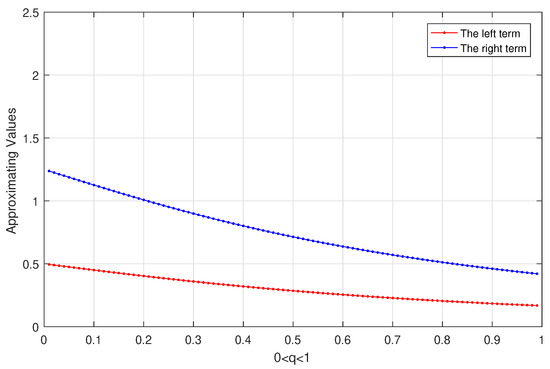
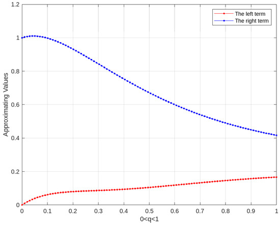
The right side of inequality (7) becomes

$$\begin{array}{cc}\hfill \left[{\displaystyle \frac{f\left(a\right)+f\left(b\right)}{2}}+{\displaystyle \frac{1}{4}}\left(\eta \left(f\right(a),f(b\left)\right)+\eta \left(f\right(b),f(a\left)\right)\right)\right]{\int }_a^{b}g\left(x\right){}_a{d}_{q}x& ={\displaystyle \frac{5}{4}}{\int }_0^1{x}^2{}_0{d}_{q}x={\displaystyle \frac{5}{4(1+q+q^2)}}\hfill \end{array}$$

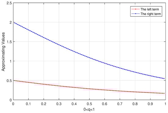
and the right side of the inequality (8) becomes

$$\begin{array}{cc}\hfill {\displaystyle \frac{f\left(a\right)+f\left(b\right)}{2}}& {\int }_a^{b}g\left(x\right){}_a{d}_{q}x+{\displaystyle \frac{1}{2}}\left[{\displaystyle \frac{\eta \left(f\right(a),f(b\left)\right)+\eta \left(f\right(b),f(a\left)\right)}{b-a}}\right]{\int }_a^b(x-a)g\left(x\right){}_a{d}_{q}x\hfill \\ \hfill & ={\displaystyle \frac{1}{2}}{\int }_0^1{x}^2{}_0{d}_{q}x+{\displaystyle \frac{1}{2}}\left[{\displaystyle \frac{\eta (0,1)+\eta (1,0)}{1-0}}\right]{\int }_0^1\left(x\right)x^2{}_0{d}_{q}x\hfill \\ \hfill & ={\displaystyle \frac{1}{2}}\left({\displaystyle \frac{1}{1+q+q^2}}\right)+{\displaystyle \frac{1}{2}}\left({\displaystyle \frac{1+2}{1}}\right)\left({\displaystyle \frac{1}{1+q+q^2+q^3}}\right)\hfill \\ \hfill & ={\displaystyle \frac{1}{2}}\left({\displaystyle \frac{1}{1+q+q^2}}\right)+{\displaystyle \frac{3}{2}}\left({\displaystyle \frac{1}{1+q+q^2+q^3}}\right).\hfill \end{array}$$

We use Matlab software to calculate the left term and right term, as shown in Figure 1 and Figure 2, which demonstrates the results described in inequalities (7) and (8) of Theorem 2.

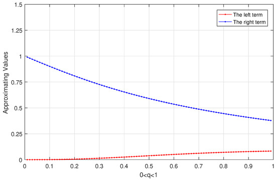
From Theorem 2, the left side of inequality (9) becomes

$$\begin{array}{cc}\hfill {\int }_a^{b}f(a+b-x)g\left(x\right){}_a{d}_{q}x& ={\int }_0^1(1-x)x^2{}_0{d}_{q}x\hfill \\ \hfill & ={\int }_0^1{x}^2{}_0{d}_{q}x-{\int }_0^1{x}^3{}_0{d}_{q}x\hfill \\ \hfill & ={\displaystyle \frac{1}{1+q+q^2}}-{\displaystyle \frac{1}{1+q+q^2+q^3}},\hfill \end{array}$$

and the right side of inequality (9) becomes

$$\begin{array}{cc}\hfill {\displaystyle \frac{f\left(a\right)+f\left(b\right)}{2}}& {\int }_a^{b}g{\left(x\right)}_a{d}_{q}x+{\displaystyle \frac{\eta \left(f\right(a),f(b\left)\right)}{2(b-a)}}{\int }_a^b(x-a)g\left(x\right){}_a{d}_{q}x+{\displaystyle \frac{\eta \left(f\right(b),f(a\left)\right)}{2(b-a)}}{\int }_a^b(b-x)g\left(x\right){}_a{d}_{q}x\hfill \\ \hfill & ={\displaystyle \frac{1}{2}}{\int }_0^1{x}^2{}_0{d}_{q}x+{\displaystyle \frac{1}{2}}{\int }_0^1{x}^3{}_0{d}_{q}x+{\int }_0^1{x}^2-x^3{}_0{d}_{q}x\hfill \\ \hfill & ={\displaystyle \frac{3}{2}}{\int }_0^1{x}^2{}_0{d}_{q}x-{\displaystyle \frac{1}{2}}{\int }_0^1{x}^3{}_0{d}_{q}x\hfill \\ \hfill & ={\displaystyle \frac{3}{2(1+q+q^2)}}-{\displaystyle \frac{1}{2(1+q+q^2+q^3)}}.\hfill \end{array}$$

We use Matlab software to calculate the left term and right term, as shown in Figure 3, which demonstrates the results described in inequality (9) of Theorem 2.

Example 5.

Define functions $f:[0,1]\to \mathbb{R}$ by $f\left(x\right)=x$ and $g:[0,1]\to {\mathbb{R}}^{+}$ by $g\left(x\right)={(2x-1)}^2$. Consider a bifunction $\eta :{\mathbb{R}}^{+}\times {\mathbb{R}}^{+}\to {\mathbb{R}}^{+}$ as

$$\eta (x,y)=\left\{\begin{array}{cc}x+y,\hfill & \mathit{for}x\le y;\hfill \\ 2(x+y),\hfill & \mathit{for}x>y.\hfill \end{array}\right.$$

Then f is an η-convex function and g is symmetric about $x=(a+b)/2$.

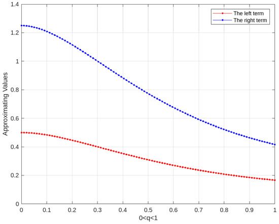
From Theorem 3, the left side of inequalities (19) becomes

$$\begin{array}{cc}\hfill {\displaystyle \frac{1}{2}}\left[{\int }_a^{b}f\left(x\right)g\left(x\right){}_a{d}_{q}x+{\int }_a^{b}f\left(x\right)g\left(x\right){}^b{d}_{q}x\right]& ={\displaystyle \frac{1}{2}}\left[{\int }_0^{1}x{(2x-1)}^2{}_0{d}_{q}x+{\int }_0^{1}x{(2x-1)}^2{}^1{d}_{q}x\right]\hfill \\ \hfill & ={\displaystyle \frac{1}{2}}\left[{\int }_0^{1}4x^3-4x^2+x{}_0{d}_{q}x+{\int }_0^{1}4x^3-4x^2+x{}^1{d}_{q}x\right]\hfill \\ \hfill & ={\displaystyle \frac{1}{2}}[\left(4{\int }_0^1{x}^3{}_0{d}_{q}x-4{\int }_0^1{x}^2{}_0{d}_{q}x+{\int }_0^{1}x{}_0{d}_{q}x\right)\hfill \\ \hfill & +\left(4{\int }_0^1{x}^3{}^1{d}_{q}x-4{\int }_0^1{x}^2{}^1{d}_{q}x+{\int }_0^{1}x{}^1{d}_{q}x\right)]\hfill \\ \hfill & ={\displaystyle \frac{1}{2}}\left(1-{\displaystyle \frac{4}{1+q}}+{\displaystyle \frac{4}{1+q+q^2}}\right),\hfill \end{array}$$

and the right side of inequality (19) becomes

$$\begin{array}{cc}\hfill & \left[{\displaystyle \frac{f\left(a\right)+f\left(b\right)}{2}}+{\displaystyle \frac{1}{4}}\left(\eta \left(f\right(a),f(b\left)\right)+\eta \left(f\right(b),f(a\left)\right)\right)\right]{\int }_a^{b}g\left(x\right){}_a{d}_{q}x\hfill \\ \hfill & =\left[{\displaystyle \frac{f\left(0\right)+f\left(1\right)}{2}}+{\displaystyle \frac{1}{4}}\left(\eta \left(f\right(0),f(1\left)\right)+\eta \left(f\right(1),f(0\left)\right)\right)\right]{\int }_0^1{(2x-1)}^2{}_0{d}_{q}x\hfill \\ \hfill & =\left[{\displaystyle \frac{1}{2}}+{\displaystyle \frac{1}{4}}(1+2)\right]{\int }_0^{1}4x^2-4x+1{}_0{d}_{q}x\hfill \\ \hfill & ={\displaystyle \frac{5}{4}}\left({\displaystyle \frac{4}{1+q+q^2}}-{\displaystyle \frac{4}{1+q}}+1\right).\hfill \end{array}$$

We use Matlab software to calculate the left term and right term, as shown in Figure 4, which demonstrates the results described in inequality (19) of Theorem 3.

From Theorem 3, the left side of inequalities (20) becomes

$$\begin{array}{cc}\hfill {\int }_a^{b}f\left(x\right)g\left(x\right){}^b{d}_{q}x& ={\int }_0^{1}x{(2x-1)}^2{}^1{d}_{q}x\hfill \\ \hfill & ={\int }_0^{1}4x^3-4x^2+x{}^1{d}_{q}x\hfill \\ \hfill & =4{\int }_0^1{x}^3{}^1{d}_{q}x-4{\int }_0^1{x}^2{}^1{d}_{q}x+{\int }_0^{1}x{}^1{d}_{q}x\hfill \\ \hfill & =1-{\displaystyle \frac{5}{1+q}}+{\displaystyle \frac{8}{1+q+q^2}}-{\displaystyle \frac{4}{1+q+q^2+q^3}},\hfill \end{array}$$

and the right side of inequality (20) becomes

$$\begin{array}{cc}\hfill & {\displaystyle \frac{f\left(a\right)+f\left(b\right)}{2}}{\int }_a^{b}g{\left(x\right)}_a{d}_{q}x\hfill \\ \hfill & +{\displaystyle \frac{1}{2(b-a)}}\left[\eta (f\left(a\right),f\left(b\right)){\int }_a^b(x-a)g\left(x\right){}_a{d}_{q}x+\eta (f\left(b\right),f\left(a\right)){\int }_a^b(x-a)g\left(x\right){}^b{d}_{q}x\right].\hfill \\ \hfill & ={\displaystyle \frac{f\left(0\right)+f\left(1\right)}{2}}{\int }_0^1{(2x-1)}^2{}_0{d}_{q}x\hfill \\ \hfill & +{\displaystyle \frac{1}{2(1-0)}}\left[\eta (f\left(0\right),f\left(1\right)){\int }_0^{1}x{(2x-1)}^2{}_0{d}_{q}x+\eta (f\left(1\right),f\left(0\right)){\int }_0^{1}x{(2x-1)}^2{}^1{d}_{q}x\right]\hfill \\ \hfill & ={\displaystyle \frac{1}{2}}\left({\displaystyle \frac{4}{1+q+q^2}}-{\displaystyle \frac{4}{1+q}}+1\right)+{\displaystyle \frac{1}{2}}\left(2-{\displaystyle \frac{9}{1+q}}+{\displaystyle \frac{12}{1+q+q^2}}-{\displaystyle \frac{4}{1+q+q^2+q^3}}\right).\hfill \end{array}$$

We use Matlab software to calculate the left term and right term, as shown in Figure 5, which demonstrates the result described in inequality (20) of Theorem 3.

5. Conclusions

The convexity of a function is a basis for many inequalities in mathematics. It should be noted that in new problems related to convexity, a general idea of the convex function is required to obtain relevant results. One of these overviews is the concept of the $\eta$-convex function, which can be summarized by many inequalities associated with convex functions, especially the famous Fejér inequality, by evaluating the difference between the left and middle terms and between the right and middle terms of this inequality. Moreover, we derived some new quantum analogues of Hermite–Hadamard–Fejér-type inequalities for $\eta$-convex functions. It is expected that this paper may stimulate further research in this field.

References

1. Jackson, F.H. On a q-definite integrals. Quart. J. Pure. Appl. Math. 1910, 41, 193–203. [Google Scholar]
2. Jackson, F.H. q-difference equations. Am. J. Math. 1910, 32, 305–314. [Google Scholar] [CrossRef]
3. Bangerezaka, G. Variational q-calculus. J. Math. Anal. Appl. 2004, 289, 650–665. [Google Scholar] [CrossRef] [Green Version]
4. Annyby, H.M.; Mansour, S.K. q-Fractional Calculus and Equations; Springer: Helidelberg, Germany, 2012. [Google Scholar]
5. Ernst, T. A Comprehensive Treatment of q-Calculus; Springer: Basel, Switzerland, 2012. [Google Scholar]
6. Ernst, T. A History of q-Calculus and a New Method; UUDM Report; Uppsala University: Uppsala, Sweden, 2000. [Google Scholar]
7. Gauchman, H. Integral inequalities in q-calculus. J. Comput. Appl. Math. 2002, 47, 281–300. [Google Scholar] [CrossRef] [Green Version]
8. Kac, V.; Cheung, P. Quantum Calculus; Springer: New York, NY, USA, 2002. [Google Scholar]
9. Tariboon, J.; Ntouyas, S.K. Quantum calculus on finite intervals and applications to impulsive difference equations. Adv. Differ. Equ. 2013, 2013, 282. [Google Scholar] [CrossRef] [Green Version]
10. Tariboon, J.; Ntouyas, S.K. Quantum integral inequalities on finite intervals. J. Inequal. Appl. 2014, 2014, 121. [Google Scholar] [CrossRef] [Green Version]
11. Bermudo, S.; Korus, P.; Napoles Valdes, J.E. On q-Hermite–Hadamard inequalities for general convex functions. Acta Math. Hungar. 2020, 162, 364–374. [Google Scholar] [CrossRef]
12. Fejér, L. Über die fourierreihen. Math. Naturwiss. Anz Ungar. Akad. Wiss. 1906, 24, 369–390. [Google Scholar]
13. Chen, F.; Wu, S. Fejér and Hermite–Hadamard type inequalities for harmonically convex functions. J. Appl. Math. 2014, 2014, 386806. [Google Scholar] [CrossRef] [Green Version]
14. Huy, V.N.; Chung, N.T. Some generalizations of the Fejér and Hermite–Hadamard inequalities in Holder spaces. J. Appl. Math. Inform. 2011, 29, 859–868. [Google Scholar]
15. Sarikaya, M.Z. On new Hermite Hadamard Fejér type integral inequalities. Stud. Univ. Babes-Bolyai Math. 2012, 57, 377–386. [Google Scholar]
16. Arunrat, N.; Nakprasit, K.M.; Nonlaopon, K.; Tariboon, J.; Ntouyas, S.K. On Fejér-type inequalities via (p,q)-calculus. Symmetry 2021, 13, 953. [Google Scholar] [CrossRef]
17. Mehmood, S.; Mehmood, H.M.; Mohammed, P.O.; Mohammed, E.A.; Zafar, F.; Nonlaopon, K. Fejér-type midpoint and trapezoidal inequalities for the operator ω1,ω2-preinvex functions. Axioms 2023, 12, 16. [Google Scholar] [CrossRef]
18. Latif, M.A. Some companions of Fejér-type inequalities using GA-convex functions. Mathematics 2023, 11, 392. [Google Scholar] [CrossRef]
19. Delavar, M.R.; De La Sen, M. On generalization of Fejér-type inequalities. Commun. Math. Appl. 2017, 8, 31–43. [Google Scholar]
Figure 1. Plot illustration for the left term and the right term for inequality (7).
Mathematics 11 03387 g001
Figure 2. Plot illustration for the left term and the right term for inequality (8).
Mathematics 11 03387 g002
Figure 3. Plot illustration for the left term and the right term for inequality (9).
Mathematics 11 03387 g003
Figure 4. Plot illustration for the left term and the right term for inequality (19).
Mathematics 11 03387 g004
Figure 5. Plot illustration for the left term and the right term for inequality (20).
Mathematics 11 03387 g005
Disclaimer/Publisher’s Note: The statements, opinions and data contained in all publications are solely those of the individual author(s) and contributor(s) and not of MDPI and/or the editor(s). MDPI and/or the editor(s) disclaim responsibility for any injury to people or property resulting from any ideas, methods, instructions or products referred to in the content.