Abstract
In the Design of Experiments, we seek to relate response variables to explanatory factors. Response Surface methodology (RSM) approximates the relation between output variables and a polynomial transform of the explanatory variables using a linear model. Some researchers have tried to adjust other types of models, mainly nonlinear and nonparametric. We present a large panel of Machine Learning approaches that may be good alternatives to the classical RSM approximation. The state of the art of such approaches is given, including classification and regression trees, ensemble methods, support vector machines, neural networks and also direct multi-output approaches. We survey the subject and illustrate the use of ten such approaches using simulations and a real use case. In our simulations, the underlying model is linear in the explanatory factors for one response and nonlinear for the others. We focus on the advantages and disadvantages of the different approaches and show how their hyperparameters may be tuned. Our simulations show that even when the underlying relation between the response and the explanatory variables is linear, the RSM approach is outperformed by the direct neural network multivariate model, for any sample size (<50) and much more for very small samples (15 or 20). When the underlying relation is nonlinear, the RSM approach is outperformed by most of the machine learning approaches for small samples (n ≤ 30).
MSC:
62J02
1. Introduction
Design of Experiments (DoE) is used in any manufacturing process where, on the one hand, input parameters called factors affect a process or a formula and can be controlled, and on the other hand, output parameters of this process, which therefore represent the results, are called responses. For example, input parameters can be a temperature or a pH, and output parameters can be a yield or an impurity rate. Experiments must be performed to determine a relationship between factors and responses. DoE allows us to select these experiments in such a way that the position of the experimental points in the space to be studied is optimal. In particular, spatial modeling can be used to better understand the process and to predict the variation of responses throughout the variation range of the factors. In these experiments, responses and factors may be quantitative, qualitative, or a mix of both. The number of experiments is often very small, because each may need several days or even weeks, and the cost can be considerable. Among the important tasks that are used in the DoE approach, response surface methodology (RSM) estimates the values of all responses for any combination of factors’ values. This is achieved by means of a regression of the responses on the factors. The most common approach considers each response separately and then uses polynomial regression, including or excluding interactions between factors. Polynomial regression suffers from several limitations, as follows: (i) the model is linear in the coefficients; (ii) to get a good approximation of the surfaces, higher degrees of polynomials may be necessary together with interactions, and this considerably increases the number of variables to include in the model and therefore the number of experiments to be performed; (iii) the model may only be estimated if the number of experiments is larger than the number of factors included in the model; and (iv) polynomial models are inappropriate in the case of nonlinear systems [1].
Several papers have suggested machine learning (ML) approaches as an alternative to polynomial regression. The approaches that are considered in the literature include Support Vector Machines (SVM) [1,2,3,4,5,6], Neural Networks (NN) [1,2,4,6,7,8,9], Random Forests (rf) [1,3,4,10], Boosting and its extension [1,3], Extra Tree regression (ET) [3,4] and Classification And Regression Trees (CART) [1]. In these papers, the authors compared some of these approaches only on real datasets, using specific settings with respect to the nature and dimensions of the data. As well as focusing on a specific dataset, the comparisons considered very few approaches at the same time and were based on very different metrics. In this work, we will mainly consider the contribution of ML with respect to the RSM; these approaches have been shown to be very efficient in various fields, such as ecology [11] and epidemiology [12].
In this paper, we give a state of the art of the ML approaches that have often been used as alternatives to polynomial regression in RSM, including direct multi-output approaches. We will briefly describe these approaches and compare them using simulation models in various situations with different sample sizes and over a real DoE case study. The simulations were actually limited to numerical variables; including categorical ones as input or output did not have any significant effect on our main results or conclusions. The advantage and the contribution of our work lies, on one hand, in the choices of the simulations; some responses are in favor of the RSM approach and others are not. On the other hand, to our knowledge, direct multivariate output approaches have never been used in this context.
This paper is organized as follows. Section 2 gives a summary of the polynomial RSM-based approach and a brief description of the most well-known ML approaches. Section 3 gives the state of the art for the applications of these approaches in various domains where DoE is practiced. In Section 4, we compare all of the ML approaches to polynomial regression on simulated multiple output datasets, varying sample sizes and optimizing the models’ hyperparameters. A real dataset is used for similar experiments. The last section includes our discussions and conclusion.
2. Response Surface Methodology
Among the many objectives of experimental design, Response Surface Methodology (RSM) [13] is used to determine the value of one or more outputs at any point in the experimental domain of interest [14] without carrying out an infinite number of experiments. This is achieved using a regression model of the form:
where f is the unknown regression function. To estimate f, we need to make some hypothesis about its shape. Polynomial models are most commonly used to address this issue. Using high-degree polynomials, f may be approximated correctly. This is a linear model in the coefficients. With K factors and degree d, the number of coefficients of the model is . According to the type of study, polynomial models of degree 1 or 2 are used because the number of observations is, in general, very small (often less than 20).
Let be the original K controlled factors, which are also called the natural variables, whose space is called the experimental domain. These variables are generally on different scales, and they may bias the modeling results. Thus, they are often normalized and linearly transformed into codified variables , which are dimensionless quantities and with the same range. The most commonly used transformation is , where is called the central value and is the step. The transformed variables lie in the interval , and the matrix is called the experimental design, where n is the sample size. A polynomial model of degree 2 may be written as:
where Y is the response and are the unknown coefficients. Once the design of the experiments is carried out and the data are available, the coefficients of the model are estimated by ordinary least squares, and their estimate is given by:
where is the model matrix, is the transpose of X, Y is the response, is the information matrix, and is the dispersion matrix.
Test points may be used to validate the model, or an analysis of the variance may be performed. After validation, the model is used to predict the variation of responses throughout the experimental domain represented by a response surface (Figure 1). These predictions can then be used to construct a Design Space, which is a region in which the response specifications will be achieved with a fixed probability [15]. Nevertheless, due to the small sample sizes available in experimental designs, polynomial models of degree 2 may give very poor estimation for surface responses.
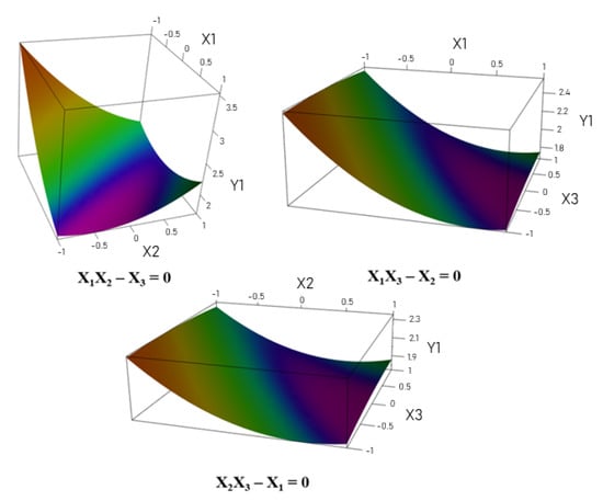
Figure 1.
Example of surface responses [16].
Alternative models have been proposed for several years. ML models present more flexible methods of estimating a response surface function: they are nonparametric and nonlinear models, and may even be efficient when the number of experiments is small compared to the number of factors.
3. Machine Learning Approaches
In this section, we will give a brief description of the most commonly used approaches in ML, as follows: k-nearest neighbors (knn), CART, Ensemble models (Bagging, Boosting, and rf), SVM, and NN.
3.1. knn
This is one of the simplest ML approaches that may be used in regression and in classification [17]. It is also quite different from all of the other approaches, in that the model estimation and prediction are embedded. Once the number of neighbors k is fixed, for any new observation x, the method seeks its k nearest neighbors within the learning set. The prediction for x is the average of the neighbors’ outputs in regression, or the majority vote in classification. The decision rule may be refined using, for instance, weighted averages or weighted majority votes, where weights may be inversely proportional to the distances of the neighbors from x. Note that the distance used to identify neighbors is a hyperparameter for this approach, together with k.
3.2. CART
Classification and Regression Trees [18] are based on recursive partitioning of the input space using rectangles. These partitions are represented by a sequence of binary splitting rules of the form , where is one of the input variables and s is a threshold over it. The split at each stage of the partitioning is optimized by an exhaustive search looking for the couple variable and threshold that minimizes the heterogeneity of the obtained subsamples. Heterogeneity is measured with respect to the output y. When the output is continuous, the deviance is used (the variance multiplied by the sample size). For discrete output, entropy or Gini criteria are used.
CART is is the most popular nonlinear and nonparametric method when one wants to understand how the model relates the outputs to the explanatory variables. It is one of the few methods which is graphically representable.
3.3. Ensemble Methods
The idea of ensemble methods, in their simplest approach, is to build K bootstrap samples of the dataset at hand, adjust a model chosen from within a class of functions (e.g., decision trees) for each bootstrap sample (denoted ), and then use the K models for predictions. In regression, the prediction by the ensemble is a weighted average of the K predictions given from each . In classification, it is a weighted majority vote over the K predictions given by the models .
Several variants of ensemble methods exist, differing either in the way in which the bootstrap samples are generated, in the estimation of each , in the way in which the individual models are combined, or in the algorithm used to estimate the whole process.
Random Forests (rf; [19] are among the most well-known and used approaches. This approach combines trees built over bootstrap samples by simple averages in regression and majority vote in classification. The trees that are built in rf may be very big, because they are not optimized, and the choice of the splits at each node in the trees is made on a small subset of variables chosen at random. Because bootstrap samples are independent, random forests may be parallelized.
Boosting [20] is quite different because the trees built over bootstrap samples are obtained sequentially; weights are associated to each observation in the original dataset, and at each step of the algorithm, a tree is built and tested over the original dataset. Observations whose prediction at step k is wrong will have their weight increased. The modified weights are used at the next step for the next bootstrap sample. Each tree that is built in the ensemble has a weight related to its performance, and the final output is a weighted majority vote in classification and a weighted average in regression. The trees’ estimates and their weights may be obtained using a gradient approach, as is applied in the gradient boosting method (gbm) [21].
Extreme gradient boosting (xgboost [22]) is another gradient boosting algorithm, which employs some additional tricks to estimate the parameters (i.e., trees and their weights). The optimization is carried out globally at the level of each split in the different trees and, as in rf, splits are optimized over a randomly sampled subset of covariates. The loss function optimized in the algorithm uses regularization over the weights and, optionally, a shrinkage of each tree added to the ensemble.
3.4. Support Vector Machines
Support vector machines [23] seek a linear separation of observations, like linear regression, but minimize a loss function based on the margins. In binary classification, the optimal regression is the hyper-plane, which perfectly separates the two classes and stays the farthest distance possible from its nearest points from the two classes. This hyper-plane may be easily found if the classes are linearly separable. If they are not, then the dataset is projected using nonlinear transformations in a much higher space where linear separation may be guaranteed. The linear transformations that are used in this case are expressed using kernel functions, among which the most commonly used are polynomial and radial kernels. These kernels, together with the optimization algorithm used to find the optimal hyper-plane, depend in general on several hyperparameters that must be fixed or tuned by the user. We will denote svmPoly (resp. svmRadial) as the support vector regression using polynomial (resp. radial) kernel.
Support Vector Machines may show high performance when the data are linearly separable, and are very efficient for large datasets. They also have a very solid mathematical justification.
3.5. Neural Networks
NNs, and specifically multi-layer perceptron (mlp) [17], are designed to handle multiple outputs. An mlp is composed of successive layers, each having a fixed number of neurons. Each neuron of a layer receives information (its inputs) from all of the neurons of the previous layers and outputs a nonlinear transformation of a linear combination of its inputs. In Figure 2, the left-hand panel shows a simple neuron having d inputs . This neuron will output the value:
where the are the weights , , and is a nonlinear function. The right-hand panel in Figure 2 shows an mlp with one hidden layer containing three neurons. Various types of layers may also be used to design a NN. We shall mainly use the fully connected layers (also called dense layers).

Figure 2.
Left-hand panel: a neuron with d inputs. Right-hand panel: a NN with a one-dimensional input and output, and one hidden layer containing three neurons.
Once the structure of the network is specified (number of layers and number of neurons per layer), all of the weights of the NN that are unknown are estimated. To achieve this, a loss function should be specified (mean squared error for regression), together with an optimization algorithm (typically gradient-based algorithms). In some situations, specific activation layers are added to the networks, mainly for the last layer (softmax for multi-class learning, sigmoid for multi-label learning).
Neural networks are among the most difficult to tune because of the large number of hyperparameters that may be involved in the structure of the network and in the choice of the optimization algorithms. For small datasets, they may be unstable due to random initializations of the weights within the training.
3.6. Multidimensional Output Approaches
In many situations, the output variable to be predicted may be multidimensional in dimension q; multi-target regression, multi-label learning, distribution learning, semantic segmentation (for images), or time series. Various approaches may be used to tackle this situation. Direct multi-output regression is the simplest approach, which consists of using one model per output component. In this case, one assumes that the output components are independent. Chained regression is another approach that accounts for dependence among output variables. The output variables should first be ranked, and one model is learnt for each output, as follows: for output variable j, the original explanatory variables X are used as input, together with the predictions of all of the outputs already modelled. In this approach, the result depends strongly on the order used for the responses.
Some supervised learning algorithms also have the ability to jointly consider the q output variables within the same model, which is the case for the example of NN, and also regression trees [24].
In classical regression trees, the output variable y is used to compute the deviance, that is, the splitting criterion of a node t:
where is the empirical mean of y in node t (which corresponds to a subset of the original sample). When y is multidimensional, , the deviance is easily generalized [24]:
where stands for the Euclidean norm in . In this case, the values assigned to each node and each leaf of the tree are the q dimensional vectors . The rest of the algorithm is similar to the one-dimensional output. We will denote this approach as .
The main advantage of direct multiple-output approaches is that they may account for dependencies between the different outputs. and its variants have been widely used in various applications.
3.7. Hyperparameters and Their Tuning
The performance of any ML algorithm highly depends on the choice of its hyperparameters. Each approach uses several hyperparameters, from one to almost ten. In most cases, these parameters have to be optimized, which is often achieved using cross-validation. Tuning may require excessive computation times, depending on the number of hyperparameters to be adjusted. Details about the tuning process and the hyperparameters used will be given in the experiments section.
3.8. Metrics Used to Compare the Models
Analysis of variance is generally used to evaluate the performance of polynomial models in RSM. Depending on the problem under study, it can be observed that the variation in outputs may not be due to the variation in inputs. Different criteria may be used to assess and compare the accuracy of the prediction obtained using any regression model. Let n be the size of the sample used to evaluate the models, be the observed value of the response for observation i, be the average of responses in the sample, and be the predicted value of the response for observation i. Among the most used metrics, we can find:
- Root Mean Square Error,
- Mean Absolute Error,
- Mean Absolute Percentage Error,
- Determination Coefficient,
- Akaike Information Criterion, , where k is the number of parameters to be estimated in the model and L is the maximum likelihood function of the model
Other, less well-known or used metrics also appear in the literature:
- The explained variance by the model is the proportion of the variance due to the factors,
- The Nash and Sutcliffe Efficiency is equivalent to the but uses absolute differences rather than quadratic,
- The agreement index d is a standardized measure of the degree of model prediction error,
- The average absolute deviations from a central point (this metric is defined and used in [8], but the name given by the authors does not seem appropriate for us as it is not in line with their definition),
The objective is to minimize , , , , and , and to maximize , , , and d. The results encountered in the literature show that, in general, when different metrics are used for comparisons, they are very often concordant with respect to the objectives.
When the output y is multidimensional, any of these criteria may be used by computing its average over all the dimensions.
4. Comparisons between RSM and ML Approaches
A comparison of these response surface models with ML has been made, mainly in the field of mechanics and materials development.
ML models were compared to the traditional RSM polynomial approximation on a mechanical engineering case study [1]. The authors studied 63 continuous factors and 8 continuous responses combined to produce a one-dimensional output, with 56,512 observations. Polynomial models of degree 1 and 2, Least Absolute Shrinkage Selection Operator [25], Generalized Linear Model [26] and nonlinear ML models (Random Forest, Gradient Boosting Decision Tree [17], Multiple Layer Perceptrons and Support Vector Regression) were tested. Three evaluation criteria were used for the comparisons, as follows: Explained Variance (EV), Mean Absolute Percentage Error (MAPE) and Root Mean Square Error (RMSE). The results obtained show that all ML models outperform the polynomial models of the RSM approach. The authors also note that for larger training set sizes, nonlinear ML models were more accurate. A simulation of the data by the MC method is proposed to improve the estimation of the response surface function. Comparisons made in this work are based on a real dataset with large samples; the true underlying relation between the response and the factors is unknown. Meanwhile, eight original responses were combined to get a one-dimensional output.
In [2], ML models were used to predict coating thickness in a nonlinear electrostatic spray deposition process and compared with the conventional RSM model. Three continuous factors and one continuous response were considered with 30 observations. A polynomial model of degree 2 (RSM), NN (Back-Propagation algorithm [27]) and Support Vector Machine models were used. MAPE was calculated to evaluate the performance of these models. The results suggest that the SVM model gives the best prediction accuracy.
The objective of [3] was to predict the viscosity of nano-polymers used in an enhanced oil recovery method, using the response surface methodology and supervised machine learning approaches. Five continuous factors and one continuous response were available, with 57 observations. The authors applied a polynomial model of degree 2 and analysis of variance, which did not show inadequacy for this model. However, the covariance matrix analysis showed that there is no linear relationship between the factors. Therefore, the authors also used nonlinear ML models, namely ridge regression [28], lasso regression, Support Vector Machine, Decision Tree, random forest, Extra tree regression [29], Gradient Boosting Regression and eXtreme Gradient Boosting [22]. Akaike Information Criterion (AIC), Mean Absolute Error (MAE), RMSE and coefficient of determination were used as evaluation and comparison criteria. The results show that the ensemble models give more accurate results than the RSM. Furthermore, the eXtreme Gradient Boosting model was the best model for response prediction.
In another study, where the objective was to predict the microhardness of a synthesized electroless Ni-P-TiO coated aluminium composite, five continuous factors and one continuous response were considered with 36 observations [4]. The authors tested a polynomial model of degree 2 and four ML models (NN, SVM, rf and Extra Trees). Mean Square Error (MSE), MAE and determination coefficient were used as evaluation criteria to compare these models. The results show that the ET model presents the lowest MSE and MAE values. This model also had the greatest .
Hybrid regression and ML models were tested to predict the ultimate condition of fiber-reinforced polymer-confined concrete [5]. The authors used an open database with eight continuous factors, two continuous responses and 765 observations. The authors compared some existing physical empirical models developed by other authors with the RSM and SVR models, together with a hybrid model combining SVR and RSM models. The following metrics were used to evaluate these models: RMSE, MAE, Nash and Sutcliffe Efficiency (NSE) and agreement index d. The authors show that the hybrid model presents a lower RMSE, lower MAE, higher NSE and higher d than other models.
Similar comparisons with ML approaches may also be found in other fields, such as pharmaceutical development. Ref. [6] worked on the effect of the core/shell technique on improving powder compactability. In this paper, two continuous factors, two binary factors and two continuous responses were measured in 28 experiments. The authors used the RSM approach, adjusting one model for each combination of the two binary factors levels, thus, four models for each response. For the ML approach, the authors compared an SVR model and four types of NN models: Backpropagation Neural Network (BPNN), Genetic Algorithm Based BPNN (GA-BPNN) [30], Mind Evolutionary Algorithm Based BPNN (MEA-BPNN) [31]), and Extreme Learning Machine (ELM) [32]. The evaluation criteria were the variance coefficient of the RMSE and RMSE for all models, and AIC for NN models only. The results show that NN models provide better prediction accuracy than other models.
The objective of the authors of [10] was to apply RSM and ML combined with data simulation to estimate metal recovery from freshwater sediments. In this work, three continuous factors were studied, six continuous responses were measured and 18 experiments were carried out. A polynomial model of degree 2 was estimated and used for data simulation. ML models, namely Lazy KStar [33] and rf algorithms, were also tested. A comparison of the models was made by means of RMSE and coefficient of determination. The results show that RSM models overestimate the observed responses by 19% compared to ML models.
Ref. [8] compared RSM and ML approaches (NN) to predict the efficient extraction of artemisinin (a precursor molecule of the most powerful antimalarial drugs on the market). In this work, three continuous factors were studied, one continuous response was measured and a central composite design was constructed with 20 experiments. For the RSM approach, ANOVA was calculated and shows that the variability of the response cannot be adequately predicted by the RSM model depending on the factors studied. This result can be explained by a complex relationship between variables. Multiple Layer Perceptrons (feed forward NN) were also tested. A comparison between these two models was performed by means of Absolute Average Deviation (AAD). The authors concluded that the NN model has better prediction accuracy.
Ref. [9] analysed NN models as an alternative modeling technique for datasets showing nonlinear relationships, using data from a tablet compression study. In this work, six continuous factors were studied, two continuous responses were measured, and 102 experiments were performed. The authors calculated a polynomial model of degree 2 with only important terms (p-value < 0.05) for the RSM approach and calculated a “generalized feed forward multiple layer perceptron network” for the ML approach. A comparison of the determination coefficients of these two models suggests that the NN model can more accurately predict the variation of the response.
A summary of these papers comparing RSM and ML approaches is given in Table 1.

Table 1.
Summary of RSM vs. ML studies—PM: Polynomial Model, LASSO: Least Absolute Shrinkage Selection Operator, GLM: Generalized Linear Model, rf: random forest, GBDT: Gradient Boosting Decision Tree, MLP: Multiple Layer Perceptrons, SVR: Support Vector Regression, BPNN: Back-Propagation Neural Network, SVM: Support Vector Machine, CART: Classification and Regression Tree, ET: Extra Tree regression, GBR: Gradient Boosting Regression, xgboost: eXtreme Gradient Boosting, NN: Neural Network, GA-BPNN: Genetic Algorithm-Back Propagation Neural Network, MEA-BPNN: Mind Evolutionary Algorithm Based BPNN, ELM: Extreme Learning Machine, EV: Explained Variance, MAPE: Mean Absolute Percentage Error, RMSE: Root Mean Square Error, AIC: Akaike Information Criterion, MAE: Mean Absolute Error, : coefficient of determination, MSE: Mean Square Error, NSE: Nash and Sutcliffe Efficiency, d: agreement index, CV RMSE: Coefficient of Variance of the RMSE, AAD: Absolute Average Deviation.
5. Experiments
In this section, we compare all of the ML approaches described in Section 3 to the polynomial model over a simulated dataset and a real dataset. We describe the datasets that we used, and how the different models are tuned and compared. All of the experiments were conducted using R software together with the RStudio Team [34] and the package “caret” [35].
5.1. Simulated Model
The simulated model that we use is based on two independent continuous factors, and , following a uniform distribution over . The three responses—denoted as , , and —are computed as follows:
where is a random noise with zero mean and standard deviation . The responses were chosen deliberately to present various types of function, as follows: polynomial of degree 2 (), nonlinear (), and nonlinear with discontinuities (). A graphical representation of these responses is shown in Figure 3.
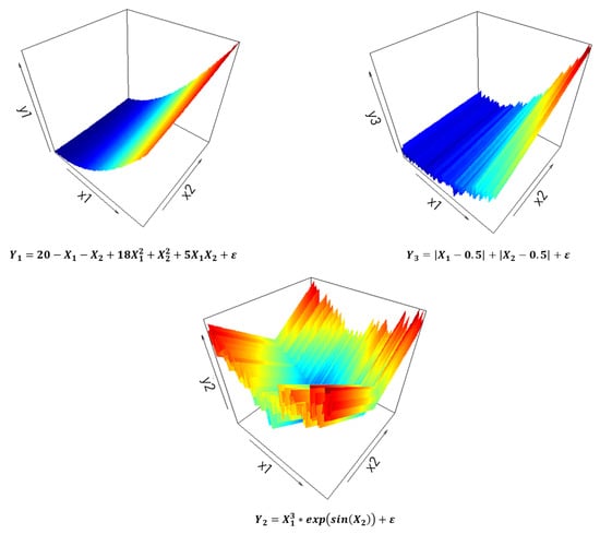
Figure 3.
Response surfaces of the simulated model.
Using this simulated model, we generated a training sample of size n and a test sample of the same size. Different values of n were tested, as follows: 15, 20, 30 and 50 observations. Small samples were used for conformity with true DoE applications. For each simulated dataset of size n, we computed the RMSE metric. Simulations were repeated times, and RMSE values were averaged over the different runs. We also varied the variance of the random noise, testing two values, and .
5.1.1. Tuning the Models
We compared the RSM approach with all of the ML approaches described in Section 3: knn, CART, rf, gbm, xgboost, svmPoly, svmRadial, NN, CARTmv and NNmv. The models were trained using the model matrix as input, thus, the true factors together with their squares and interactions.
All ML models depend on several hyperparameters. To optimize the values of the hyperparameters, we applied the grid search approach. Thus, a grid was defined for each model’s hyperparameter, and three-fold cross-validation with five repeats was used for the optimization. The optimal values of the hyperparameters were then used to learn the model over the training set and evaluate it on the test sample. Table 2 lists the hyperparameters for each method, together with a short description and the grid used for its optimization.
Table 2.
Hyperparameter values tested for each method. knn: k-nearest neighbors, rf: random forest, svmPoly: support vector machine with polynomial kernel, svmRadial: support vector machine with radial basis function kernel, CART: Classification And Regression Tree, gbm: gradient boosting machine, xgboost: eXtreme Gradient Boosting, NN: Neural Network, CARTmv: Classification and Regression Tree with multivariate responses, NNmv: Neural Network with multivariate responses.
The average of the optimal values of the hyperparameters and their standard deviation for each approach and each response are given in Appendix A.1.
5.1.2. Results
Table 3, Table 4, Table 5 and Table 6 show the average and standard deviation of the RMSE scores computed over the test samples for each response and averaged over repetitions (columns, , and ), and the average RMSE over the responses (column ). We also reported the rank of each model with respect to its RMSE for each response (, and ) and for the average over responses (). A model has rank 1 for a response if it has the smallest RMSE, and thus, is the best. Each table corresponds to a different sample size n. Boxplots of the RMSE over the runs for all the models and the outputs are shown in Appendix A.2.
Table 3.
RMSE and rank for each method and each response (n = 50). Gray cells highlight the best model.
Table 4.
RMSE and rank for each method and each response (n = 30). Gray cells highlight the best model.
Table 5.
RMSE and rank for each method and each response (n = 20). Gray cells highlight the best model.
Table 6.
RMSE and rank for each method and each response (n = 15). Gray cells highlight the best model.
For (Table 3), the best models for the three responses were multivariate NN (for ), svm with polynomial kernel (for ) and NN (for ). The linear model had positions (2, 5, 5).
For (Table 4), the best models for the three responses were, respectively: multivariate NN (for ) and NN (for and ). With respect to the average of all response errors, svm with polynomial kernel is the best model in this case. Linear regression is at position 2 for , but at position 8 for the other two responses. These first results seem to be in agreement with the state of the art: ML approaches may provide better prediction estimates for the responses.
We obtained similar results for smaller sample sizes, (Table 5), and (Table 6): multivariate NN (for ), knn (for ) and NN (for ) were the best models. Linear regression gets the worst results as the sample size decreases, particularly for and , which are nonlinear responses.
Globally, the RSM approach seems to be inefficient when compared to ML approaches, mainly with small sample sizes and for responses that are originally nonlinear in the factors. Even for large samples (, compared to what is available in DoE), RSM is outperformed in our experiments for linear response. Finally, multivariate NNs show excellent performance in various situations, mainly for the linear response () where they outperform the RSM for any sample size.
5.2. Use Case
We used the pharmaceutical application that is described in [16]. This article is based on the development of the high-performance liquid chromatography analytical method to quantify verapamil hydrochloride (which is a chemical molecule involved in headaches) and its impurities in tablets. In this use case, three continuous factors (buffer pH, ammonium hydroxide concentration in mobile phase and injection volume of test solutions) and five continuous responses (capacity factor for the first eluted peak denoted , resolution between two impurities denoted , signal-to-noise for an impurity denoted , resolution between two other impurities denoted , and retention time difference between oxidative impurity peak and the closest impurity denoted ) were available. The authors used the RSM approach to determine optimal chromatographic conditions.
For the real case study, we conducted similar experiments as for the simulated dataset, replacing random generation with random splitting. Thus, for each of the 50 repetitions, the original dataset was randomly split using proportions and for learning and testing, respectively. The results that we obtained are given in Table 7. The best models with respect to the RMSE were xgb for , gbm for , multivariate NN for , NN for and knn for . For the overall error, multivariate NN had the smallest error. For this real dataset, and for all responses, ML models gave better results than the RSM approach.
Table 7.
RMSE and rank for each method and each response (DOE case study). Gray cells highlight the best model.
6. Conclusions
In this work, using extensive simulations and a real use case, we have demonstrated that ML approaches present a very interesting alternative to response surface modeling in the DoE. We have tested a large panel of ML approaches, together with direct multi-output regression models (decision trees and NNs), which had never previously been used in this context. Clearly, various ML approaches outperformed RSM in all our experiments. RSM is very simple to use compared to ML approaches, due to the fact that several hyperparameters must be tuned correctly in ML algorithms. This requires optimization procedures over grids. The caret package is a good wrapper for this task and for most of the approaches that we have used, except for multi-output regression, where we implemented the grid search algorithm directly. Another constraint of caret is that not all the hyperparameters involved in each approach may be tuned, and thus it may be necessary to use other packages for this issue.
In our implementation, we used the factors together with their squares and interactions in the ML approaches. Very few papers are clear about this choice. We also tested the models including only the factors, and in some cases a loss in performance appeared for some ML algorithms, but the main conclusion was observed: several ML approaches outperformed classical RSM.
Many ML and deep learning approaches were not explored in this work (like [36,37,38,39]) and may have some advantages and drawbacks compared to those we have used. Due to the very large choice of such approaches, it is impossible to be exhaustive, so we have selected the ones most used and cited in the literature. In addition, further higher-polynomial-order factors could be included as input in the different models. Together with feature selection approaches, this may give better performance for various ML approaches.
Author Contributions
Conceptualization, B.G. and D.M.; methodology, B.G. and D.M.; software, D.M.; validation, B.G. and D.M.; formal analysis, B.G. and D.M.; investigation, B.G. and D.M.; resources, B.G. and D.M.; writing—original draft preparation, B.G. and D.M.; writing—review and editing, B.G. and D.M.; visualization, B.G. and D.M.; supervision, B.G.; project administration, D.M. All authors have read and agreed to the published version of the manuscript.
Funding
This research received no external funding.
Data Availability Statement
On request by email.
Acknowledgments
The authors gratefully acknowledge Claude Deniau and Sophie Declomesnil for their constructive comments on the manuscript.
Conflicts of Interest
The authors declare no conflict of interest.
Appendix A. Supplementary Material
Appendix A.1. Mean and Standard Deviation of Hyperparameter Values
In each of the runs, the optimized values of the parameters were computed. The following tables give the mean and standard deviation of the hyperparameters for each response.
Table A1.
Average and standard deviation (SD) of the hyperparameters for all responses with and .
Table A1.
Average and standard deviation (SD) of the hyperparameters for all responses with and .
| Hyperparameters | Average Y1 | SD Y1 | Average Y2 | SD Y2 | Average Y3 | SD Y3 |
|---|---|---|---|---|---|---|
| k | 4.06 | 1.268 | 9.34 | 2.21 | 8.4 | 2.304 |
| minsplit | 3 | 2.474 | 1.3 | 1.199 | 1.2 | 0.99 |
| minbucket | 1.8 | 1.852 | 5.4 | 1.641 | 5.6 | 1.37 |
| cp | 0.003 | 0.002 | 0.023 | 0.011 | 0.018 | 0.012 |
| minsize | 5.46 | 3.382 | 5.54 | 3.57 | 5.44 | 3.144 |
| mtry | 3.2 | 0.7 | 2.3 | 0.839 | 2.64 | 1.208 |
| n.trees | 93 | 58.038 | 50 | 0 | 54 | 28.284 |
| interaction.depth | 1.96 | 0.88 | 1.08 | 0.34 | 1.08 | 0.396 |
| shrinkage | 0.1 | 0 | 0.1 | 0 | 0.1 | 0 |
| n.minobsinnode | 10 | 0 | 10 | 0 | 10 | 0 |
| nrounds | 70 | 47.38 | 50 | 0 | 51 | 7.071 |
| max_depth | 1.2 | 0.495 | 1.36 | 1.064 | 1.12 | 0.521 |
| eta | 0.3 | 0 | 0.306 | 0.024 | 0.304 | 0.02 |
| gamme | 0 | 0 | 0 | 0 | 0 | 0 |
| colsample_bytree | 0.712 | 0.1 | 0.684 | 0.1 | 0.664 | 0.094 |
| min_child_weight | 1 | 0 | 1 | 0 | 1 | 0 |
| subsample | 0.743 | 0.178 | 0.828 | 0.187 | 0.833 | 0.197 |
| degree | 1.32 | 0.653 | 1.76 | 0.87 | 1.42 | 0.758 |
| scale | 2.312 | 3.661 | 0.141 | 0.292 | 0.412 | 1.977 |
| 1.66 | 1.358 | 1.535 | 1.445 | 0.48 | 0.756 | |
| sigma | 0.537 | 0.42 | 0.525 | 0.515 | 0.497 | 0.503 |
| 5.08 | 7.359 | 0.35 | 0.196 | 0.46 | 1.1 | |
| layer1 | 4.96 | 1.355 | 5.04 | 1.525 | 3.64 | 1.549 |
| layer2 | 5.12 | 1.223 | 4.64 | 1.306 | 3.64 | 1.601 |
| layer3 | 4.92 | 1.523 | 5.04 | 1.355 | 3.72 | 1.715 |
| minsplit | 2.8 | 2.424 | 2.8 | 2.424 | 2.8 | 2.424 |
| minbucket | 2.4 | 2.268 | 2.4 | 2.268 | 2.4 | 2.268 |
| cp | 0.006 | 0.006 | 0.006 | 0.006 | 0.006 | 0.006 |
| layer1 | 4 | 1.512 | 4 | 1.512 | 4 | 1.512 |
| layer2 | 4.04 | 1.484 | 4.04 | 1.484 | 4.04 | 1.484 |
| layer3 | 3.92 | 1.712 | 3.92 | 1.712 | 3.92 | 1.712 |
Table A2.
Average and standard deviation (SD) of the hyperparameters for all responses with and .
Table A2.
Average and standard deviation (SD) of the hyperparameters for all responses with and .
| Hyperparameters | Average Y1 | SD Y1 | Average Y2 | SD Y2 | Average Y3 | SD Y3 |
|---|---|---|---|---|---|---|
| k | 3.08 | 1.047 | 8.28 | 2.241 | 8.52 | 2.297 |
| minsplit | 1.9 | 1.94 | 1.1 | 0.707 | 1.3 | 1.199 |
| minbucket | 1.3 | 1.199 | 5.7 | 1.199 | 5.7 | 1.199 |
| cp | 0.006 | 0.006 | 0.013 | 0.011 | 0.013 | 0.013 |
| minsize | 5.6 | 3.169 | 5.64 | 3.269 | 5.04 | 3.597 |
| mtry | 3.78 | 1.016 | 2.22 | 0.737 | 2.34 | 0.917 |
| n.trees | 113 | 62.93 | 57 | 26.745 | 51 | 7.071 |
| interaction.depth | 1.58 | 0.499 | 1.28 | 0.454 | 1.26 | 0.443 |
| shrinkage | 0.1 | 0 | 0.1 | 0 | 0.1 | 0 |
| n.minobsinnode | 10 | 0 | 10 | 0 | 10 | 0 |
| nrounds | 106 | 73.29 | 68 | 51.27 | 51 | 7.071 |
| max_depth | 2.06 | 1.449 | 1.86 | 1.414 | 1.74 | 1.44 |
| eta | 0.31 | 0.03 | 0.318 | 0.039 | 0.322 | 0.042 |
| gamme | 0 | 0 | 0 | 0 | 0 | 0 |
| colsample_bytree | 0.704 | 0.101 | 0.656 | 0.091 | 0.684 | 0.1 |
| min_child_weight | 1 | 0 | 1 | 0 | 1 | 0 |
| subsample | 0.69 | 0.189 | 0.745 | 0.197 | 0.735 | 0.198 |
| degree | 1.4 | 0.639 | 1.56 | 0.787 | 1.66 | 0.895 |
| scale | 1.824 | 3.359 | 0.139 | 0.293 | 0.252 | 1.421 |
| 1.555 | 1.226 | 1.135 | 1.292 | 0.995 | 1.243 | |
| sigma | 0.397 | 0.27 | 0.518 | 0.635 | 0.494 | 0.339 |
| 6.16 | 6.973 | 0.68 | 2.24 | 0.345 | 0.214 | |
| layer1 | 4.96 | 1.228 | 4.64 | 1.588 | 3.68 | 1.684 |
| layer2 | 5.52 | 0.953 | 4.96 | 1.228 | 4.24 | 1.791 |
| layer3 | 5.32 | 1.186 | 4.04 | 1.784 | 4.12 | 1.637 |
| minsplit | 2.7 | 2.393 | 2.7 | 2.393 | 2.7 | 2.393 |
| minbucket | 1.5 | 1.515 | 1.5 | 1.515 | 1.5 | 1.515 |
| cp | 0.009 | 0.008 | 0.009 | 0.008 | 0.009 | 0.008 |
| layer1 | 4.12 | 1.637 | 4.12 | 1.637 | 4.12 | 1.637 |
| layer2 | 3.88 | 1.686 | 3.88 | 1.686 | 3.88 | 1.686 |
| layer3 | 4.28 | 1.512 | 4.28 | 1.512 | 4.28 | 1.512 |
Table A3.
Average and standard deviation (SD) of the hyperparameters for all responses with and .
Table A3.
Average and standard deviation (SD) of the hyperparameters for all responses with and .
| Hyperparameters | Average Y1 | SD Y1 | Average Y2 | SD Y2 | Average Y3 | SD Y3 |
|---|---|---|---|---|---|---|
| k | 2.88 | 0.849 | 8.3 | 2.485 | 8.54 | 2.786 |
| minsplit | 1.8 | 1.852 | 1.7 | 1.753 | 1.7 | 1.753 |
| minbucket | 1 | 0 | 4.7 | 2.215 | 5.2 | 1.852 |
| cp | 0.005 | 0.005 | 0.012 | 0.012 | 0.006 | 0.009 |
| minsize | 5.58 | 3.308 | 5.24 | 3.384 | 4.48 | 3.209 |
| mtry | 4.08 | 1.007 | 2.62 | 1.159 | 2.34 | 0.848 |
| n.trees | 72 | 55.476 | 51 | 7.071 | 59 | 40.013 |
| interaction.depth | 1 | 0 | 1 | 0 | 1 | 0 |
| shrinkage | 0.1 | 0 | 0.1 | 0 | 0.1 | 0 |
| n.minobsinnode | 10 | 0 | 10 | 0 | 10 | 0 |
| nrounds | 110 | 74.231 | 62 | 38.545 | 59 | 34.538 |
| max_depth | 2.72 | 1.356 | 2.26 | 1.601 | 1.68 | 1.332 |
| eta | 0.324 | 0.043 | 0.32 | 0.04 | 0.32 | 0.04 |
| gamme | 0 | 0 | 0 | 0 | 0 | 0 |
| colsample_bytree | 0.716 | 0.1 | 0.656 | 0.091 | 0.68 | 0.099 |
| min_child_weight | 1 | 0 | 1 | 0 | 1 | 0 |
| subsample | 0.67 | 0.169 | 0.75 | 0.192 | 0.725 | 0.192 |
| degree | 1.32 | 0.621 | 1.58 | 0.758 | 1.26 | 0.6 |
| scale | 2.33 | 3.652 | 0.488 | 1.975 | 0.223 | 1.411 |
| 1.415 | 1.173 | 1.675 | 1.581 | 0.675 | 0.892 | |
| sigma | 0.308 | 0.222 | 0.323 | 0.219 | 0.695 | 1.371 |
| 7 | 9.318 | 0.455 | 0.562 | 0.485 | 0.64 | |
| layer1 | 4.76 | 1.333 | 4.08 | 1.614 | 3.68 | 1.731 |
| layer2 | 5.36 | 1.174 | 4.44 | 1.68 | 4.04 | 1.641 |
| layer3 | 5.6 | 0.808 | 3.52 | 1.644 | 4.08 | 1.85 |
| minsplit | 2.1 | 2.092 | 2.1 | 2.092 | 2.1 | 2.092 |
| minbucket | 1 | 0 | 1 | 0 | 1 | 0 |
| cp | 0.01 | 0.01 | 0.01 | 0.01 | 0.01 | 0.01 |
| layer1 | 3.92 | 1.563 | 3.92 | 1.563 | 3.92 | 1.563 |
| layer2 | 4.2 | 1.471 | 4.2 | 1.471 | 4.2 | 1.471 |
| layer3 | 3.88 | 1.48 | 3.88 | 1.48 | 3.88 | 1.48 |
Table A4.
Average and standard deviation (SD) of the hyperparameters for all responses with and .
Table A4.
Average and standard deviation (SD) of the hyperparameters for all responses with and .
| Hyperparameters | Average Y1 | SD Y1 | Average Y2 | SD Y2 | Average Y3 | SD Y3 |
|---|---|---|---|---|---|---|
| k | 2.74 | 0.853 | 7.16 | 2.691 | 7.84 | 2.985 |
| minsplit | 1.2 | 0.99 | 1.4 | 1.37 | 1.7 | 1.753 |
| minbucket | 1.1 | 0.707 | 4.8 | 2.157 | 4.5 | 2.315 |
| cp | 0.008 | 0.009 | 0.005 | 0.007 | 0.005 | 0.008 |
| minsize | 5.72 | 3.084 | 6.32 | 3.365 | 6.48 | 3.346 |
| mtry | 4.52 | 0.863 | 2.66 | 1.099 | 2.5 | 1.055 |
| n.trees | 107 | 90.356 | 81 | 70.631 | 55 | 29.014 |
| interaction.depth | 1 | 0 | 1 | 0 | 1 | 0 |
| shrinkage | 0.1 | 0 | 0.1 | 0 | 0.1 | 0 |
| n.minobsinnode | 10 | 0 | 10 | 0 | 10 | 0 |
| nrounds | 115 | 76.432 | 62 | 42.33 | 68 | 52.255 |
| max_depth | 2.6 | 1.539 | 2.52 | 1.581 | 2.76 | 1.611 |
| eta | 0.314 | 0.035 | 0.332 | 0.047 | 0.336 | 0.048 |
| gamme | 0 | 0 | 0 | 0 | 0 | 0 |
| colsample_bytree | 0.728 | 0.097 | 0.652 | 0.089 | 0.664 | 0.094 |
| min_child_weight | 1 | 0 | 1 | 0 | 1 | 0 |
| subsample | 0.72 | 0.185 | 0.68 | 0.194 | 0.685 | 0.188 |
| degree | 1.16 | 0.468 | 1.7 | 0.814 | 1.32 | 0.683 |
| scale | 2.492 | 3.814 | 0.872 | 2.726 | 0.257 | 1.42 |
| 1.715 | 1.489 | 1.175 | 1.311 | 0.74 | 1.087 | |
| sigma | 0.262 | 0.184 | 0.346 | 0.23 | 0.489 | 0.55 |
| 3.5 | 3.066 | 1.435 | 3.188 | 1.51 | 3.361 | |
| layer1 | 4.52 | 1.446 | 3.92 | 1.614 | 4.04 | 1.784 |
| layer2 | 5.32 | 1.186 | 4.72 | 1.604 | 4.52 | 1.607 |
| layer3 | 5.44 | 0.993 | 3.48 | 1.798 | 3.72 | 1.807 |
| minsplit | 2.3 | 2.215 | 2.3 | 2.215 | 2.3 | 2.215 |
| minbucket | 1.2 | 0.99 | 1.2 | 0.99 | 1.2 | 0.99 |
| cp | 0.007 | 0.007 | 0.007 | 0.007 | 0.007 | 0.007 |
| layer1 | 4.04 | 1.641 | 4.04 | 1.641 | 4.04 | 1.641 |
| layer2 | 4.12 | 1.586 | 4.12 | 1.586 | 4.12 | 1.586 |
| layer3 | 4.64 | 1.367 | 4.64 | 1.367 | 4.64 | 1.367 |
Table A5.
Average and standard deviation (SD) of the hyperparameters for all responses of DoE case study.
Table A5.
Average and standard deviation (SD) of the hyperparameters for all responses of DoE case study.
| Hyperparameters | Average Y1 | SD Y1 | Average Y2 | SD Y2 | Average Y3 | SD Y3 | Average Y4 | SD Y4 | Average Y5 | SD Y5 |
|---|---|---|---|---|---|---|---|---|---|---|
| k | ||||||||||
| minsplit | ||||||||||
| minbucket | ||||||||||
| cp | ||||||||||
| minsize | ||||||||||
| mtry | ||||||||||
| n.trees | ||||||||||
| interaction.depth | ||||||||||
| shrinkage | ||||||||||
| n.minobsinnode | ||||||||||
| nrounds | ||||||||||
| max_depth | ||||||||||
| eta | ||||||||||
| gamma | ||||||||||
| colsample_bytree | ||||||||||
| min_child_weight | ||||||||||
| subsample | ||||||||||
| degree | ||||||||||
| scale | ||||||||||
| sigma | ||||||||||
| layer1 | ||||||||||
| layer2 | ||||||||||
| layer3 | ||||||||||
| minsplit | ||||||||||
| minbucket | ||||||||||
| cp.1 | ||||||||||
| layer1 | ||||||||||
| layer2 | ||||||||||
| layer3 |
Appendix A.2. Boxplots of Errors for All Approaches and Responses

Figure A1.
Response Y1: R = 50, n = 50, sd = 1.
Figure A1.
Response Y1: R = 50, n = 50, sd = 1.


Figure A2.
Response Y2: R = 50, n = 50, sd = 1.
Figure A2.
Response Y2: R = 50, n = 50, sd = 1.


Figure A3.
Response Y3: R = 50, n = 50, sd = 1.
Figure A3.
Response Y3: R = 50, n = 50, sd = 1.


Figure A4.
Response Y1: R = 50, n = 30, sd = 1.
Figure A4.
Response Y1: R = 50, n = 30, sd = 1.


Figure A5.
Response Y2: R = 50, n = 30, sd = 1.
Figure A5.
Response Y2: R = 50, n = 30, sd = 1.


Figure A6.
Response Y3: R = 50, n = 30, sd = 1.
Figure A6.
Response Y3: R = 50, n = 30, sd = 1.


Figure A7.
Response Y1: R = 50, n = 20, sd = 1.
Figure A7.
Response Y1: R = 50, n = 20, sd = 1.


Figure A8.
Response Y1: R = 50, n = 20, sd = 1.
Figure A8.
Response Y1: R = 50, n = 20, sd = 1.


Figure A9.
Response Y3: R = 50, n = 20, sd = 1.
Figure A9.
Response Y3: R = 50, n = 20, sd = 1.


Figure A10.
Response Y1: R = 50, n = 15, sd = 1.
Figure A10.
Response Y1: R = 50, n = 15, sd = 1.


Figure A11.
Response Y2: R = 50, n = 15, sd = 1.
Figure A11.
Response Y2: R = 50, n = 15, sd = 1.


Figure A12.
Response Y3: R = 50, n = 15, sd = 1.
Figure A12.
Response Y3: R = 50, n = 15, sd = 1.


Figure A13.
Response Y1: DOE case study—R = 50.
Figure A13.
Response Y1: DOE case study—R = 50.


Figure A14.
Response Y2: DOE case study—R = 50.
Figure A14.
Response Y2: DOE case study—R = 50.


Figure A15.
Response Y3: DOE case study—R = 50.
Figure A15.
Response Y3: DOE case study—R = 50.


Figure A16.
Response Y4: DOE case study—R = 50.
Figure A16.
Response Y4: DOE case study—R = 50.


Figure A17.
Response Y5: DOE case study—R = 50.
Figure A17.
Response Y5: DOE case study—R = 50.

References
- Zhang, Y.; Wu, Y. Introducing Machine Learning Models to Response Surface Methodologies. In Response Surface Methodology in Engineering Science; IntechOpen: London, UK, 2021. [Google Scholar]
- Paturi, U.M.R.; Reddy, N.S.; Cheruku, S.; Narala, S.K.R.; Cho, K.K.; Reddy, M.M. Estimation of coating thickness in electrostatic spray deposition by machine learning and response surface methodology. Surf. Coat. Technol. 2021, 422, 127559. [Google Scholar] [CrossRef]
- Lashari, N.; Ganat, T.; Otchere, D.; Kalam, S.; Ali, I. Navigating viscosity of GO-SiO2/HPAM composite using response surface methodology and supervised machine learning models. J. Pet. Sci. Eng. 2021, 205, 108800. [Google Scholar] [CrossRef]
- Shozib, I.A.; Ahmad, A.; Rahaman, M.A.; Alam, M.; Beheshti, M.; Taufiqurrahman, I. Modelling and optimization of microhardness of electroless Ni-P-TiO2 composite coating based on machine learning approaches and RSM. J. Mater. Res. Technol. 2021, 12, 1010–1025. [Google Scholar] [CrossRef]
- Keshtegar, B.; Gholampour, A.; Thai, D.K.; Taylan, O.; Trung, N.T. Hybrid regression and machine learning model for predicting ultimate condition of FRP-confined concrete. Compos. Struct. 2021, 262, 113644. [Google Scholar] [CrossRef]
- Lou, H.; Chung, J.I.; Kiang, Y.H.; Xiao, L.Y.; Hageman, M.J. The application of machine learning algorithms in understanding the effect of core/shell technique on improving powder compactability. Int. J. Pharm. 2019, 555, 368–379. [Google Scholar] [CrossRef]
- Haque, S.; Khan, S.; Wahid, M.; Dar, S.A.; Soni, N.; Mandal, R.K.; Singh, V.; Tiwari, D.; Lohani, M.; Areeshi, M.Y.; et al. Artificial Intelligence vs. Statistical Modeling and Optimization of Continuous Bead Milling Process for Bacterial Cell Lysis. Front. Microbiol. 2016, 7, 1852. [Google Scholar] [CrossRef]
- Pilkington, J.L.; Preston, C.; Gomes, R.L. Comparison of response surface methodology (RSM) and artificial neural networks (ANN) towards efficient extraction of artemisinin from Artemisia annua. Ind. Crops Prod. 2014, 58, 15–24. [Google Scholar] [CrossRef]
- Bourquin, J.; Schmidli, H.; van Hoogevest, P.; Leuenberger, H. Advantages of Artificial Neural Networks (ANNs) as alternative modelling technique for data sets showing non-linear relationships using data from a galenical study on a solid dosage form. Eur. J. Pharm. Sci. 1998, 7, 5–16. [Google Scholar] [CrossRef] [PubMed]
- Souza Lima, E.; Lima, V.; Almeida, C.; Justi, K. Application of response surface methodology and machine learning combined with data simulation to metal determination of freshwater sediment. Water Air Soil Pollut. 2017, 228, 370. [Google Scholar] [CrossRef]
- Bi, Q.; Goodman, K.E.; Kaminsky, J.; Lessler, J. What is Machine Learning? A Primer for the Epidemiologist. Am. J. Epidemiol. 2019, 188, 2222–2239. [Google Scholar] [CrossRef]
- Crisci, C.; Terra, R.; Pacheco, J.; Ghattas, B.; Bidegain, M.; Goyenola, G.; Lagomarsino, J.; Méndez, G.; Mazzeo, N. Multi-model approach to predict phytoplankton biomass and composition dynamics in a eutrophic shallow lake governed by extreme meteorological events. Ecol. Model. 2017, 360, 80–93. [Google Scholar] [CrossRef]
- Myers, R.H.; Montgomery, D.C.; Anderson-Cook, C.M. Response Surface Methodology: Process and Product in Optimization Using Designed Experiments; John Wiley and Sons: New York, NY, USA, 1995. [Google Scholar]
- Sarabia, L.; Ortiz, M. 1.12—Response Surface Methodology. In Comprehensive Chemometrics; Brown, S.D., Tauler, R., Walczak, B., Eds.; Elsevier: Oxford, UK, 2009; pp. 345–390. [Google Scholar] [CrossRef]
- Manzon, D.; Claeys-Bruno, M.; Declomesnil, S.; Carité, C.; Sergent, M. Quality by Design: Comparison of Design Space construction methods in the case of Design of Experiments. Chemom. Intell. Lab. Syst. 2020, 200, 104002. [Google Scholar] [CrossRef]
- dos Moreira, C.S.; Lourenço, F.R. Development and optimization of a stability-indicating chromatographic method for verapamil hydrochloride and its impurities in tablets using an analytical quality by design (AQbD) approach. Microchem. J. 2020, 154, 104610. [Google Scholar] [CrossRef]
- Hastie, T.; Tibshirani, R.; Friedman, J.; Franklin, J. The elements of statistical learning: Data mining, inference, and prediction. Math. Intell. 2004, 27, 83–85. [Google Scholar] [CrossRef]
- Breiman, L.; Friedman, J.; Stone, C.J.; Olshen, R.A. Classification and Regression Trees; Chapman and Hall/CRC: Boca Raton, FL, USA, 1984. [Google Scholar]
- Breiman, L. Random Forests. Mach. Learn. 2001, 45, 5–32. [Google Scholar] [CrossRef]
- Freund, Y.; Schapire, R.E. A decision-theoretic generalization of on-line learning and an application to boosting. J. Comput. Syst. Sci. 1997, 55, 119–139. [Google Scholar] [CrossRef]
- Natekin, A.; Knoll, A. Gradient boosting machines, a tutorial. Front. Neurorobot. 2013, 7, 21. [Google Scholar] [CrossRef]
- Chen, T.; He, T. xgboost: eXtreme Gradient Boosting. 2021. Available online: https://cran.r-project.org/web/packages/xgboost/vignettes/xgboost.pdf (accessed on 27 July 2023).
- Cristianini, N.; Shawe-Taylor, J. An Introduction to Support Vector Machines and Other Kernel-Based Learning Methods; Cambridge University Press: Cambridge, UK, 2000. [Google Scholar] [CrossRef]
- Nerini, D.; Durbec, J.; Mante, C.; Garcia, F.; Ghattas, B. Forecasting physicochemical variables by a classification tree method: Application to the Berre Lagoon (South France). Acta Biotheor. 2001, 48, 181–196. [Google Scholar] [CrossRef]
- Tibshirani, R. Regression shrinkage and selection via the Lasso. J. R. Stat. Soc. Ser. B (Methodol.) 1996, 58, 267–288. [Google Scholar] [CrossRef]
- Nelder, J.A.; Wedderburn, R.W.M. Generalized linear models. J. R. Stat. Soc. Ser. (Gen.) 1972, 135, 370. [Google Scholar] [CrossRef]
- Rumelhart, D.E.; Hinton, G.E.; Williams, R.J. Learning representations by back-propagating errors. Nature 1986, 323, 533–536. [Google Scholar] [CrossRef]
- Marquardt, D.W.; Snee, R.D. Ridge regression in practice. Am. Stat. 1975, 29, 3–20. [Google Scholar] [CrossRef]
- Geurts, P.; Ernst, D.; Wehenkel, L. Extremely randomized trees. Mach. Learn. 2006, 63, 3–42. [Google Scholar] [CrossRef]
- Schaffer, J.; Whitley, D.; Eshelman, L. Combinations of genetic algorithms and neural networks: A survey of the state of the art. In Proceedings of the COGANN-92: International Workshop on Combinations of Genetic Algorithms and Neural Networks, Baltimore, MD, USA, 6 June 1992; pp. 1–37. [Google Scholar] [CrossRef]
- Jie, J.; Zeng, J.; Han, C. An extended mind evolutionary computation model for optimizations. Appl. Math. Comput. 2007, 185, 1038–1049. [Google Scholar] [CrossRef]
- Huang, G.B.; Zhu, Q.Y.; Siew, C.K. Extreme learning machine: Theory and applications. Neurocomputing 2006, 70, 489–501. [Google Scholar] [CrossRef]
- Aljazzar, H.; Leue, S. K*: A heuristic search algorithm for finding the k shortest paths. Artif. Intell. 2011, 175, 2129–2154. [Google Scholar] [CrossRef]
- RStudio Team. RStudio: Integrated Development Environment for R; RStudio, PBC: Boston, MA, USA, 2020. [Google Scholar]
- Kuhn, M. Building predictive models in R using the caret package. J. Stat. Softw. 2008, 28, 1–26. [Google Scholar] [CrossRef]
- Dai, Y.; Yang, C.; Liu, Y.; Yao, Y. Latent-Enhanced Variational Adversarial Active Learning Assisted Soft Sensor. IEEE Sens. J. 2023, 23, 15762–15772. [Google Scholar] [CrossRef]
- Zhu, J.; Jia, M.; Zhang, Y.; Deng, H.; Liu, Y. Transductive transfer broad learning for cross-domain information exploration and multigrade soft sensor application. Chemom. Intell. Lab. Syst. 2023, 235, 104778. [Google Scholar] [CrossRef]
- Jia, M.; Xu, D.; Yang, T.; Liu, Y.; Yao, Y. Graph convolutional network soft sensor for process quality prediction. J. Process Control 2023, 123, 12–25. [Google Scholar] [CrossRef]
- Liu, K.; Zheng, M.; Liu, Y.; Yang, J.; Yao, Y. Deep Autoencoder Thermography for Defect Detection of Carbon Fiber Composites. IEEE Trans. Ind. Inform. 2023, 19, 6429–6438. [Google Scholar] [CrossRef]


Disclaimer/Publisher’s Note: The statements, opinions and data contained in all publications are solely those of the individual author(s) and contributor(s) and not of MDPI and/or the editor(s). MDPI and/or the editor(s) disclaim responsibility for any injury to people or property resulting from any ideas, methods, instructions or products referred to in the content. |
© 2023 by the authors. Licensee MDPI, Basel, Switzerland. This article is an open access article distributed under the terms and conditions of the Creative Commons Attribution (CC BY) license (https://creativecommons.org/licenses/by/4.0/).