Abstract
This paper proposes a new instrumental-type estimator of quantile regression models for panel data with fixed effects. The estimator is built upon the minimum distance, which is defined as the weighted average of the conventional individual instrumental variable quantile regression slope estimators. The weights assigned to each estimator are determined by the inverses of their corresponding individual variance–covariance matrices. The implementation of the estimation has many advantages in terms of computational efforts and simplifies the asymptotic distribution. Furthermore, the paper shows consistency and asymptotic normality for sequential and simultaneous asymptotics. Additionally, it presents an empirical application that investigates the income elasticity of health expenditures.
MSC:
62-04
1. Introduction
Panel data not only captures the individual heterogeneity inherent in cross-sectional data but also offers valuable insights into the dynamics of time series data. Quantile regression effectively captures the relationship between the independent variable X and the dependent variable Y, enabling a comprehensive understanding of how covariates systematically influence the location, scale, and shape of the conditional distribution of the response. Moreover, distinguishing it from the ordinary least squares method, quantile regression does not necessitate any assumptions about the overall distribution.
The quantile regression model applied to panel data has the capability to comprehensively describe the conditional distribution of the response variable and effectively manage variability. When endogeneity is disregarded, three estimation approaches can be employed for quantile regression in panel data with fixed effects: penalty estimation, two-step estimation, and minimum distance estimation.
The penalty estimation primarily involved the addition of a penalty term to the objective function. Koenker [1] introduced a comprehensive methodology for estimating quantile regression models in longitudinal data through the utilization of regularization techniques. It was highlighted that shrinkage could offer advantages in managing the variability arising from the estimation of fixed effects parameters. The selection of the penalty maintained the linear programming structure and preserved the sparsity of the resulting design matrix. Nevertheless, the mentioned article did not provide a method for selecting the penalty parameter. Lamarche [2] theoretically demonstrated that there was an optimal penalty parameter for the penalized quantile regression in panel data with fixed effects. As mentioned earlier, the utilization of shrinkage provides several statistical and computational advantages. However, when the number of panel subjects, represented by N, is large, the calculation of this kind of penalty estimation becomes rather complicated. Building upon Koenker [1], Gu and Volgushev [3] proposed a linear quantile regression method which allowed the researcher to learn the particular group structure of the latent effects together with common parameters of interest in the model. Galvao et al. [4] formalized the properties of bootstrap inference methods for quantile regression panel data models with fixed effects. They investigated a random-weighted bootstrap and demonstrated that it could be used to construct confidence intervals and perform inference for the parameters of interest.
The primary concept behind two-step estimation is to remove the fixed effects in the initial step, followed by employing simple quantile regression on the transformed data in the second step. Canay [5] introduced a two-step estimator for quantile regression model with fixed effects. In the first step, compute , where N is the number of panel subjects and T is the number of observation times, represents the response variable for subject i at time t, denotes a vector of observable variables, represents the parameter of interest, and stands for a -consistent estimator of . Additionally, denotes the individual effect. Estimate by a quantile regression of on in the second step. Asymptotic properties of the two-step estimator were presented in the paper. It is worth noting that the two-step estimation method eliminates the fixed effects in the initial step. This approach leads to a significant reduction in the number of estimated parameters in quantile regression and avoids the need to select penalty parameters. However, compared to , the new variable has changed the meaning of the dependent variables in the original regression model, making the discussion of the large sample properties of the estimators more complex. Chen and Huo [6] revisited the estimator proposed by Canay [5] and pointed out that the bias of the estimator due to the estimation of fixed effects was erroneously omitted in his asymptotic analysis. They proposed a two-step estimation method based on smoothed quantile regression that was easy to implement. At the same time, this paper rigorously derived the asymptotic bias of the estimation method and proposed a correct statistical inference method based on bias correction.
Galvao and Wang [7] developed a novel minimum distance quantile regression (MD-QR) estimator for panel data quantile regression model. The MD-QR estimator is defined as the weighted average of the individual quantile regression slope estimators, where the weights are determined by the inverses of their corresponding individual variance–covariance matrices. The proposed estimator exhibits efficiency within the class of minimum distance estimators. Moreover, it exhibits fast computational performance, particularly for large cross-sections. However, it should be noted that based on the definition of MD-QR, the model cannot adequately accommodate time-invariant independent variables. Furthermore, the MD-QR estimator does not account for endogenous issues. Galvao et al. [8] proved that unbiased asymptotic normality of both the fixed effects quantile regression (FE-QR) and MD-QR estimators under conditions on N, T that were very close. This result represented a significant advancement in the existing theory and showed that quantile regression was applicable to the same type of panel data (in terms of N, T) as other nonlinear models.
Chernozhukov and Hansen [9,10,11] extended the results of Koenker and Bassett [12] for the quantile regression (QR) model with all exogenous variables to a model with endogeneity when instruments were available. They proposed an instrumental variable quantile regression (IVQR) estimator that appropriately modified the conventional quantile regression. In this paper, considering the endogenous problems we extend the results of Galvao and Wang [7] and Chernozhukov and Hansen [9,10,11], combining the minimum distance estimator and instrumental variable quantile regression.
With considering the endogeneity, there has been growing work at the three types of estimation. Harding and Lamarche [13] gave the instrumental variable quantile regression with fixed effects (IVFEQR) estimator to overcome the endogenous problem, where they allowed the endogenous variables to be correlated with unobserved factors affecting the response variables. Galvao and Montes-Rojas [14] also developed an instrumental variables estimator for quantile regression in panel data with fixed effects aiming to mitigate the bias caused by the presence of measurement error (endogeneity) in the model. They showed IVFEQR estimator and proposed its asymptotic properties. Galvao and Montes-Rojas [15] proposed penalized quantile regression for dynamic panel data, utilizing instrumental variables to address the endogeneity issue. Galvao [16] adapted instrumental variable approach to investigate a dynamic panel model. Harding and Lamarche [17] further explored the static fixed effect panel data model using Huasman–Taylor instrumental variables. Zhang et al. [18] studied a penalized instrumental variables quantile regression for spatial panel model with fixed effects. They shrank the individual fixed effects to a common value with a tuning parameter, aiming to control additional variability and enhance the accuracy of parameter estimation. Besstremyannaya and Golovan [19] reviewed various methods for estimating longitudinal models for quantile regression, they pointed out that method of smoothed quantile regression could be considered as a way to mitigate the asymptotic bias of the estimator in short panels. Furthermore, there has been a growing body of research focusing on quantile regression for panel data, see, e.g., [20,21,22,23,24].
In this paper, we propose a minimum distance instrumental variable quantile regression (MD-IVQR) estimator for panel data with fixed effects to resolve biased parameter estimation caused by endogenous variables and to simplify cumbersome computation caused by large N and T. The proposed estimator expands upon the minimum distance quantile regression estimator and is defined as a weighted average of the individual instrumental variable quantile regression slope estimators. The weights are determined by taking the inverses of the corresponding individual variance–covariance matrices. As a result, MD-IVQR can be constructed from a series of classical instrumental variable quantile regressions. MD-IVQR estimation splits the data into smaller parts and estimates each of them individually instead of solving a single larger optimization problem, making the approach computationally simple to implement. We also study the asymptotic properties of the MD-IVQR estimator. The consistency results for the MD-IVQR estimator are presented in Theorems 1 and 2, while the limiting distributions of MD-IVQR estimator under different assumptions are given in Theorems 3 and 4. The validity of the proposed approach is demonstrated through Monte Carlo simulations conducted under various parameter sets. We compare the bias and root mean squared error (RMSE) of the proposed estimator with those of the IVFEQR estimator developed by Harding and Lamarche [13] as well as the MD-QR estimator proposed by Galvao and Wang [7]. We also compare the computing time for the IVFEQR estimator and MD-IVQR estimator.
The remainder of the paper is structured as follows. Section 2 introduces the MD-IVQR estimator for panel data models with fixed effects. Section 3 delves into the asymptotic behavior of the MD-IVQR estimator. Section 4 provides a detailed description of the Monte Carlo experiment. In Section 5, we apply the proposed method to investigate the income elasticity of health expenditures using panel data from 166 countries between 1995 and 2016. The results of this application are presented to illustrate the effectiveness of the proposed approach. Finally, Section 6 summarizes the findings and conclusions of this study.
2. Model and Methods
2.1. Basic Model
This paper considers the following model,
where N is the number of panel subjects and T is the number of observation times, is the response variable for subject i at time t, is a vector of endogenous variables that is correlated with unobserved factors affecting the response variable, is a vector of exogenous variables, and represent the parameters of interest, and denotes the individual effect and is the error term.
It is convenient to write model (1) in matrix form as,
where is a matrix, is a matrix, is a matrix, , is a vector of ones, is the identity matrix of order N, is the vector of individual specific effects or intercepts, and is a matrix. Note that represents an incidence matrix that identifies the N distinct individuals in the sample.
We assume that the -th quantile of the error is equal to zero. We consider the following model for the -th conditional quantile functions of ,
where is the i-th column element of matrix , used to identify the individual effect .
2.2. IVFEQR Estimator
Note that the endogenous variable is correlated with the random error item , this situation will cause biased estimation. Therefore, researchers consider using instrumental variables to reduce bias, see Harding and Lamarche [13] and Galvao and Montes-Rojas [14].
The IVFEQR estimator proposed by Harding and Lamarche [13] (also referred to in Galvao and Montes-Rojas [14]) is defined as follows:
for a given positive definite matrix and solves
where denotes compact parameter set, is a vector of the available instrumental variables, is the coefficient of the instrumental variables, and is the check function and is the indicator function (see, e.g., [12]). The instrument needs to satisfy the following two conditions: (i) instruments can impact , and ; (ii) is independent of the random error.
2.3. MD-IVQR Estimator
Because of the endogeneity, we cannot eliminate the fixed effects by transforming , and to deviations from individual means to reduce the estimated parameters. That is, for instrumental variable quantile regression, we are required to deal directly with the full problem, which means when N, T and p (the dimension of dim()+dim()) are large, there are a large number of parameters that need to be estimated. Moreover, given a suitable set of values , the estimators obtained through Formula (4) essentially correspond to the FE-QR estimators ([1]). In other words, in order to obtain IVFEQR estimators, we need to calculate a series of FE-QR estimators. However, FE-QR estimator involves optimization with large number of parameters to be estimated, making the problem computationally cumbersome, and often intractable. Motivated by the practical challenges of implementing FE-QR, Galvao and Wang [7] presented an efficient minimum distance quantile regression estimator for panels with fixed effects which was simple to implement.
Inspired by Galvao and Wang [7], we propose a minimum distance instrumental variable quantile regression estimator for model (1) to reduce the bias caused by the presence of endogeneity and to simplify cumbersome computation. The proposed estimator is a weighted combination of the IVQR estimators that can be constructed from a series of conventional instrumental variable quantile regressions. Thus, the estimation approach is computationally convenient and simple to implement in many typical applications.
Let , we consider a minimum distance instrumental variable quantile regression (MD-IVQR) estimator, denoted as , which is defined as follows:
where is the IVQR estimator of slope coefficient for each individual using the time-series data, and denotes the associated variance–covariance matrix of for each individual. As we can see, the MD-IVQR estimator is defined as the weighted average of the conventional IVQR slope estimators, with weights given by the inverses of the corresponding individual variance-covariance matrices.
Specifically, the IVQR estimator is defined as follows. Define
where is any uniformly positive definite matrix, and represent the estimated coefficients of the covariates and , as well as the estimated values of individual fixed effect for each individual given , with
is a vector of the available instrument instrumental variables, which is related to but dependent on .
The IVQR estimator is given by
Moreover, obtaining the IVQR estimator involves the following three steps.
Step 1: For a given quantile , it is necessary to define a suitable set of values . This involves performing the -quantile regression of on to obtain the ordinary QR estimators of :
Step 2: Choose from the set of values| that minimizes a weighted distance function defined on , aiming to bring the value closest to zero:
where is defined in Chernozhukov and Hansen [11].
Step 3: Subsequently, the estimation of , denoted as , can be obtained.
However, in applications, the estimator , defined in (5), is infeasible unless is known for every individual. Thus, it is suggested to use the corresponding consistent estimator to replace the unknown . Then, the MD-IVQR estimator is given by
Actually, the proposed MD-IVQR estimator is a product of a simple optimization problem. Under the restrictions,
where , is a vector containing the slope coefficients for each individual i, denotes an N-vector of ones, and is vector of parameters of interest form (3). The restriction states that all the slope coefficients from different individuals are the same. The estimated value of is denoted as , where and the definition of can be found in (6). The restriction cannot be exactly satisfied, so we need to obtain its least-square solution. Thus, we consider minimizing the following quadratic optimization problem
where U is a positive definite matrix. Under independence across individuals, we can simplify U by diagonalizing it, i.e., . Thus, the above optimization can be written as
The Equation (9) can be solved using the following expression:
This solution is analogous to the MD-IVQR estimator (8), where the MD-IVQR estimator replaces with the inverse of the estimated variance-covariance matrix of the individual regression parameter, denoted as .
In addition, when takes different values, one can obtain the class of minimum distance estimators, denoted by . As mentioned in Galvao and Wang [7], the optimal weights among all the estimators in are the inverse of the asymptotic variance–covariance matrices of the slope regression quantiles. This means that the estimator defined in (8) is the most efficient estimator in . In other words, has the smallest asymptotic variance-covariance matrix among all the estimators in . For the proof of the inverse of the covariance matrices being optimal weights, see Rao [25], Serfling [26], and Hsiao [27].
3. Asymptotic Theory
Now we briefly discuss the asymptotic properties of the MD-IVQR estimator. The existence of the parameter will raise some new issues for the asymptotic analysis of estimator as N tends to infinity. We investigate the asymptotic properties of the MD-IVQR estimator when both T and N tend towards infinity, either sequentially or simultaneously. The sequential asymptotics, denoted by , is defined by taking T to infinity first, followed by . The simultaneous asymptotics, denoted by , means that T and N tend to infinity at the same time. In order to establish the asymptotic properties of the MD-IVQR estimator, we impose the following regularity conditions.
(A1) is independent across i, and i.i.d. within each i.
(A2) For all , int, and is compact and convex. Let , and .
(A3) There is a constant M such that ,,.
(A4) For each i, let be a T-vector, be a matrix, be a matrix, be a matrix and be a vector of ones. Denote , , . For each i, has full rank at each in .
(A5) has full rank at
(A6) For each i, the function is one-to-one over .
(A7) Let be the conditional distribution function of given and have conditional density . The conditional density is continuously differentiable. There exist such that and for ; there exists such that .
(A8) Given , . For each ,
(A9) Define , , there exists such that mineig , where
Conditions (A1) is commonly seen in the quantile regression literature. Condition (A2) restricts the compactness on the parameter space of . Such a condition is needed since the objective function is not convex in . Condition (A3) requires the restriction boundary conditions of the variables. Condition (A3) also guarantees that exists and has a uniform bound. Condition (A4) is sufficient for the estimates to be asymptotically normal. Condition (A5) requires that each matrix has full rank. Condition (A6) imposes that global identifiability must hold. Condition (A5) and Condition (A6) are required to carry out the direct inference but are not required in the dual approach, as discussed in Chernozhukov and Hansen [10]. Condition (A7) imposes the smoothness and boundedness of the conditional density and its derivatives. Condition (A8) is important for the parameters’ identification. Condition (A9) assures that is bounded uniformly for each i.
In applications, it is necessary to estimate the variance–covariance matrices since they are typically unknown. Since the estimation of depends on the conditional densities and the conditional densities, which are also unknown, we study the kernel estimation of the . Let and denote sequences of positive numbers (bandwidths). When T and N tend to infinity sequentially, we propose the following condition.
(A10) for some uniformly across i and as , is a bandwidth. Assume that , where exists and is nonsingular.
(A10’) for some uniformly across i and as , is a bandwidth. Assume that , where exists and is nonsingular.
Later in the paper, we will discuss examples that satisfy both conditions (A10) and (A10’).
First, we show the consistency results for the MD-IVQR estimators in Theorems 1 and 2.
Theorem 1.
Under conditions (A1)–(A8) and (A10),
as .
Theorem 2.
Under conditions (A1)–(A8) and (A10’),
as and .
The proofs of Theorems 1 and 2 can be found in Appendix A.1 and Appendix A.2, respectively.
Next, we give the limiting distributions of MD-IVQR estimator under sequential and simultaneous limits in Theorems 3 and 4. For the sequential limits, denoted by , we let T diverge to infinity first, and then . For the simultaneous limits, we denote when and .
Theorem 3.
Under conditions (A1)–(A10), as ,
where , , , , , , , , , , , and is a partition of such that is a matrix and is a matrix.
Theorem 4.
Under conditions (A1)–(A9) and (A10’), as ,
where V is defined in Theorem 3.
The proofs of Theorems 3 and 4 can be found in Appendix A.3 and Appendix A.4, respectively.
Here are some remarks of Theorems 3 and 4. First, when dim = dim, the choice of does not affect asymptotic variance, and has the simple vision
where is defined above and . This is particularly convenient since the variance formula becomes simple once the instrument is collapsed to the same dimension as .
Second, if satisfies for each i, then we can obtain as and . Following Koenker’s [28] analysis for ordinary QR, Chernozhukov and Hansen [11] gave the estimating variance that satisfied . The components of that need to be estimated include , and . They can be estimated as follows:
where , , , is a bandwidth chosen such that and as , is a kernel function.
When dim=dim, following Galvao and Wang’s [7] analysis for ordinary MD-QR, the estimating variance satisfying condition (A10’) is defined as follows:
where , is a bandwidth chosen such that and as , is defined in Kato [29].
In Theorems 3 and 4, we provide the limiting distributions for both sequential and simultaneous asymptotics. It is noteworthy that Theorems 3 and 4 demonstrate that the MD-IVQR estimator possesses the same limiting distribution in both sequential and simultaneous asymptotic scenarios. The reasons underlying this observation are explained in Galvao and Wang [7]. However, the two asymptotic properties primarily differ in terms of the divergence rates of T and N that are required. For the sequential limits asymptotics, we begin with letting T tend to infinity, followed by N. The proofs of the sequential limits entail great mathematical simplifications by drawing on the conclusions of predecessors, such as Chernozhukov and Hansen [11]. In contrast, the simultaneous asymptotics entail stringent requirements on the growth rate of T, which should tend to infinity faster than . Consequently, the proof for the simultaneous asymptotics is relatively complex.
4. Monte Carlo Simulation
The samples are generated from the following model,
where , and . In the simulations, we fix We generate and from the same distributions, which are Gaussian distribution , t distribution with 3 degrees of freedom and Chi-squared distribution with 3 degrees of freedom . In the generation process, we set and , and discard their respective first 50 observations, using the observations through T for the estimation. The design of the experiment carried here is based on Galvao [30] and Galvao [16]. As mentioned in [31], both random effects and fixed effects models exhibit endogeneity issues in dynamic panel data models because the lagged dependent variable is correlated with the disturbance, even if it is assumed that is not itself autocorrelated. Thus, we use as an instrument variable. The choice of the values of lagged one periods as an instrument variable has been used in previous studies, such as Galvao [30] and Galvao [16]. We set the number of replications to 1000.
For the sake of comparing the performance and efficiency between different methods, we compare the bias, RMSE of the following estimators: the instrumental variables estimator for quantile regression with fixed effects (IVFEQR) as in Harding and Lamarche [13]; the minimum distance quantile regression estimator (MD-QR) as in Galvao and Wang [7] and the proposed MD-IVQR estimator. In the simulations, we report results considering , , and quantiles . As the true value of is 0.5, we generate a series of values from 0.3 to 0.7 in steps of 0.01 in the estimation process. In practice, we suggest first calculating the QR or MD-QR estimator and then setting a series of values near this estimate in the initial step.
Moreover, in quantile regression, the error term follows a general distribution F, and the derivative of the quantile function is referred to as the sparsity function (see [32]). Therefore, to examine whether the finite sample performance of the estimator is affected by sparsity function estimation in the weights, we calculate both the true and estimated sparsity functions within the corresponding variance–covariance matrix for the MD-IVQR and MD-QR estimators. We denote the MD-IVQR using the true sparsity as MDIVT and the MD-IVQR using the estimated sparsity as MDIVE. For MDIVE, we estimate the variance-covariance matrix using kernel estimation with the Gaussian kernel function. Following Galvao and Wang [7], we set the bandwidth as , where represents the Hall–Sheather bandwidth. Similarly, the MD-QR using the true sparsity is denoted as MDT, while the MD-QR using the estimated sparsity is abbreviated as MDE. Given the table layout and size, we abbreviate IVFEQR as IVFE.
4.1. Bias and RMSE
Table 1 presents the bias and RMSE of the estimators for and when . In terms of the bias of , it is evident that the IVFE, MDIVE, and MDIVT estimators outperform the MDE and MDT estimators. This implies that the methods using IV yield superior estimation results. The RMSE results are consistent with the bias findings. The RMSE of the MDE and MDT estimators is generally larger than that of the other three estimators.

Table 1.
Bias and RMSE of estimators for and when .
Regarding the coefficient of the exogenous variable , the overall results obtained by the five estimators do not significantly differ from each other. However, when N and T are small, the MDE and MDT estimators perform noticeably worse than the other three estimators. Furthermore, the RMSE of the MDIVT estimator is smaller than that of MDIVE, and the RMSE of the MDT estimator is also smaller than that of MDE. Nevertheless, the impact of sparsity estimation diminishes as the sample size increases. In other words, the estimation results of MDIVE and MDIVT estimators do not vary significantly with the increase in sample size. Whether the sparsity function is estimated or known, it does not significantly affect the estimation performance as the sample size grows.
Furthermore, as noted by Galvao and Wang [7], it is observed that the bias decreases as T increases for all estimators. However, this reduction in bias does not occur as N increases due to the incidental parameter problem. For a fixed N, the bias and RMSE of the five estimators decrease as T increases. Similarly, for a fixed T, the bias and RMSE of the MDIVE and MDIVT estimators tend to decrease with an increase in N. Meanwhile, there is little disparity in the estimation effects on the parameters at different quantiles.
Table 2 displays the bias and RMSE of estimators for and when . The results are comparable to those obtained from the distribution. The MDIVE and MDIVT estimators outperform the MDE and MDT estimators, and exhibit similar performance to the IVFE estimators.
Table 2.
Bias and RMSE of estimators for and when .
Table 3 provides the the bias and RMSE of estimators for and when . The results demonstrate similarities to those obtained from the and distributions at the 0.25 and 0.5 quantiles. However, the estimation results are relatively poorer at higher quantile points.
Table 3.
Bias and RMSE of estimators for and when .
It is worth mentioning that, contrary to the findings of Galvao and Wang [7], we observe that MDIVT’s estimation results are no longer always better than MDIVE’s. The reason is that when solving the model, we first give a suitable set of values , and then we analyze the new y instead of the original model. From the above analysis, on the one hand, we can find that MDIVT is better than MDIVE in most cases, while on the other hand, the effects of sparsity estimation diminish as the sample size increases.
Finally, we conducted an analysis to assess the bias in the MDIVE estimators for as varies. Considering , and assuming , we obtained estimates of the bias in the MDIVE estimators for different values ranging from 0.2 to 0.8 with a step size of 0.05. The results of the bias estimation for the MDIVE estimators of are presented in Figure 1. Notably, the figure demonstrates that the bias falls within the range of -0.0025 to 0.0035. Additionally, it is worth mentioning that incorporating as an instrumental variable exhibited minimal impact on the bias of the MDIVE estimators across different values. These findings align with the results reported by Galvao [16].
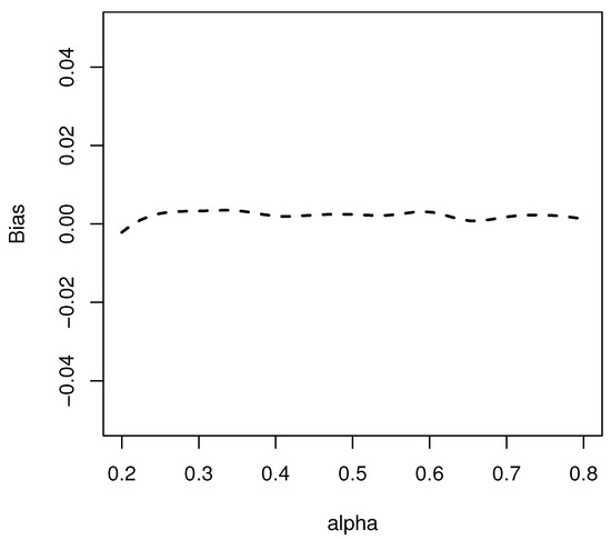
Figure 1.
Bias of the MDIVE estimators for when varies.
4.2. Estimation Speed
As discussed by Galvao and Wang [7], the estimation procedure for FE-QR models can be quite cumbersome, as is the case with IVFEQR models, which we have previously discussed. Consequently, we propose using MD-IVQR as an alternative estimator because it is both straightforward to implement and computationally feasible.
In order to compare the computing time for IVFEQR and MD-IVQR estimators, the durations of IVFEQR and MD-IVQR estimations in a simulation for various levels of N and T where we estimate the above model for one particular quantile () are presented. The code of IVFEQR is provided by Harding and Lamarche on their respective websites. We compare the time in terms of three quantities: user, system, and elapsed. User time gives the CPU time spent by the current process and system time gives the CPU time spent by the kernel (the operating system) on behalf of the current process. Elapsed time is in our best interests and gives the time charged to the CPU(s) for one replication of the simulation. In addition, the processor of computer we use is an Intel Core i5-5257U cpu@2.70 GHz RAM 8.00 GB and the program is implemented using R 3.1.1.
Table 4 illustrates the durations (in seconds) of the IVFEQR and MD-IVQR estimations in a simulation for sample sizes . From Table 4, we can see that when N, T are more than 150, the duration of MD-IVQR estimation is less than IVFEQR estimation. With the increase of N and T, the durations of MD-IVQR estimation and IVFEQR estimation both increase, and the duration of IVFEQR estimation is significantly more than that of MD-IVQR estimation. That is, the duration of MD-IVQR estimation increases slowly, while the duration of IVFEQR increases more obviously. The significant disparity in the computational time required for estimating the parameters, as discussed in Galvao and Wang [7], arises from the distinct approach employed by IVFEQR estimation and MD-IVQR estimation. IVFEQR estimation tackles a single, larger optimization problem, whereas MD-IVQR estimation subdivides the data into smaller segments and estimates them individually.
Table 4.
The durations of IVFEQR and MD-IVQR estimations in a simulation for various levels of N and T.
Furthermore, by holding N and T fixed separately, we observe whether the duration of the estimation is more sensitive to T or N. Table 5 shows the durations (in seconds) of the IVFEQR and MD-IVQR estimations in a simulation for sample sizes with fixed N. With the increase in time, T, the duration of both estimation procedures increase, but both are relatively flat. While from Table 6 with fixed T, we can see that as N increases, the duration of computing each estimator increases, although the increment is mild for MD-IVQR, it is drastic for IVFEQR. When N is greater than 250, IVFEQR consumes significantly more computing time than MD-IVQR. By comparison of Table 5 and Table 6, it can be concluded that both estimators demonstrate greater sensitivity to variations in the size of N|. In addition, MD-IVQR is much less sensitive to sample size than IVFEQR.
Table 5.
The durations of IVFEQR and MD-IVQR estimations in a simulation for various levels of T when .
Table 6.
The durations of IVFEQR and MD-IVQR estimations in a simulation for various levels of N when .
In summary, when the sample size N and time series length T are sufficiently large, IVFEQR requires substantially more computation time compared to MD-IVQR. Both estimators are more sensitive to the magnitude of N rather than T. Therefore, when dealing with a large sample, particularly for large N, it is advisable to use the MD-IVQR estimator.
5. Application
In this section, we demonstrate the effectiveness of our new approach by applying it to investigate the income elasticity of health expenditure. The substantial increase in healthcare spending has presented a challenge for many countries, and the growing proportion of healthcare expenditures as a share of GDP is an important economic trend. We apply our approach to a panel of data from 166 countries spanning from 1995 to 2016: the healthcare expenditure dataset.
The literature has extensively examined the strong and positive relationship between GDP and health expenditures. Notable studies include Newhouse [33], Gerdtham and Jönsson [34], Moran and Simon [35], Murphy and Robert [36], Farag et al. [37], Acemoglu et al. [38], and Tian et al. [39]. Farag et al. [37] employed fixed effects and instrumental variables models to investigate the income elasticity of health care spending in developed and developing countries. They noted that endogeneity may arise due to unobservable variables driving both health expenditures and income. Acemoglu et al. [38] analyzed the income elasticity of health expenditure by using global oil prices as an instrument for local area income. Their study used time-series variation in oil prices between 1970 and 1990, interacted with cross-sectional variation in oil reserves across different areas of the Southern United States.
Like Acemoglu et al. [38], the panel data model can be established as
where indicates different countries and regions, and indicates different years, denotes regional heterogeneity. Variable descriptions are summarized in Table 7. One advantage of the above modeling is that it can control the unobserved country factors. The result of Hausman test shows that the fixed effects model is preferred.
Table 7.
Variable descriptions.
To address concerns of endogeneity, we propose using instrumental variables in estimating our model, while Farag et al. [37] used the share of agriculture in the economy and primary school net enrollment ratio as instruments for income, these may not be appropriate. The primary school net enrollment ratio reflects higher national human capital and income, but also higher education levels that may lead to increased medical expenditure. Instead, following Acemoglu et al. [38], we consider using global oil prices interacted with cross-sectional oil reserves as instruments. The use of oil shocks as an instrument for GDP began with Bruckner et al. [40]. In this study, the instrument we used is the least squares projection of on the instruments and , where the total amount of oil reserves, is calculated as estimated remaining reserves plus total cumulative oil production as of 1995.
The estimation results are illustrated in Figure 2. The findings indicate that the estimated income elasticity of medical expenditure at each quantile is greater than 1, which is consistent with the results of previous studies by Newhouse [33], Gerdtham and Jönsson [34], and Murphy and Robert [36]. Furthermore, the income elasticity of medical expenditures at medium quantiles is larger than those at low and high quantiles.
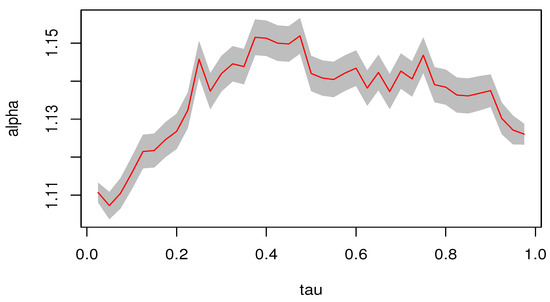
Figure 2.
The MD-IVQR estimators at different quantiles. (The shaded area in the figure represents the 95% confidence interval).
To investigate the impact of oil-rich countries on our estimation results, we exclude them from our analysis as oil price fluctuations may be influenced by their oil production. According to the BP Statistical Review of World Energy 2017, OPEC’s proven oil reserves in 2016 accounted for approximately 71.5% of the world’s total. Additionally, we divide the 166 countries in our dataset into two groups: OPEC and non-OPEC. As shown in Figure 3, the estimated income elasticity of medical expenditure for non-OPEC countries is around 1.11–1.15, consistent with the findings presented in Figure 2. Furthermore, similar to our previous results, the income elasticity of health expenditures for low and high quantiles is lower than that for medium quantiles. For OPEC countries, the estimated income elasticity of medical expenditures is mostly below 1. However, the estimates increase with the quantile.
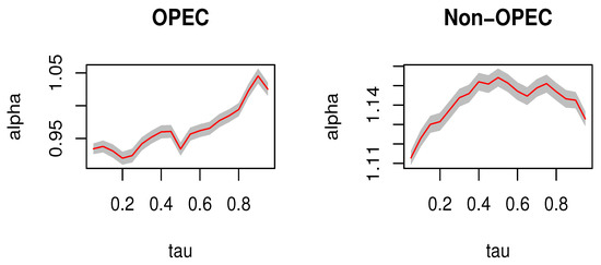
Figure 3.
The MD-IVQR estimators for OPEC and non OPEC at different quantiles. (The shaded area in the figure represents the 95% confidence interval).
To account for different stages of economic development across countries, we divide the 166 countries in our dataset into two groups: OECD and non-OECD, representing developed and developing economies, respectively. As shown in Figure 4, the estimated income elasticity of health expenditure for OECD countries is approximately 1.14–1.18, whereas for non-OECD economies, it is around 1.04–1.08. Our findings suggest that OECD countries have a relatively higher elasticity of health expenditure compared to non-OECD countries, indicating that the income elasticity of medical expenditure may increase as a country’s economic development improves. This result is consistent with the findings of Farag et al. [37], who found that healthcare spending is less responsive to changes in income in low-income countries and more responsive to changes in middle and high-income countries.
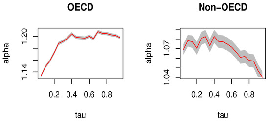
Figure 4.
The MD-IVQR estimators for OECD and non OECD at different quantiles. (The shaded area in the figure represents the 95% confidence interval).
6. Conclusions
In this paper, we propose a minimum distance instrumental variable quantile regression (MD-IVQR) estimator for panel data with fixed effects, to address the biased parameter estimation problem caused by endogenous variables and to simplify cumbersome computations due to large N and T. The MD-IVQR estimator is defined as a weighted average of conventional individual instrumental variable quantile regression slope estimators, where the weights are given by the inverses of the corresponding individual variance-covariance matrices. This estimator is a modification of the MD-QR that can be constructed from a series of conventional instrumental variable quantile regressions. The MD-IVQR estimator combines the advantages of the MD-QR estimator and the IVQR estimator, making it computationally convenient and simple to implement in many typical applications.
We give the asymptotic properties of the MD-IVQR estimator in large samples, considering both sequential and simultaneous limits. For the sequential limits asymptotics, we first let T tend to infinity, and then N. However, for the simultaneous asymptotics, we strengthen conditions and require T to tend to infinity faster than . Monte Carlo experiments show that the estimation results with the use of IV perform much better for . Furthermore, the computing time of the MD-IVQR is similar to that of IVFEQR when N and T are not large (less than 150). However, when N and T are large enough, IVFEQR consumes significantly more computing time than MD-IVQR.
Finally, we apply the proposed method to analyze the income elasticity of health expenditure. Our results indicate that the estimated income elasticity of medical expenditure at each quantile is greater than 1.
Author Contributions
Conceptualization, L.T. (Li Tao) and L.T. (Lingnan Tai); methodology, L.T. (Li Tao); software, L.T. (Li Tao); writing—original draft preparation, L.T. (Li Tao), L.T. (Lingnan Tai) and M.Q.; writing—review and editing, L.T. (Li Tao), L.T (Lingnan Tai), M.Q. and M.T.; visualization, L.T. (Li Tao); supervision, M.Q. and M.T.; funding acquisition, L.T. (Li Tao) and M.T. All authors have read and agreed to the published version of the manuscript.
Funding
Tao’s work was supported by the R&D Program of Beijing Municipal Education Commission (No. SM202210037009) and the Youth Science Fund for Beijing Wuzi University (2023XJQN04); Tian’s work was partially supported by the Fundamental Research Funds for the Central Universities and the Research Funds of Renmin University of China (22XNL016).
Data Availability Statement
The healthcare expenditure dataset in this study is available from the corresponding author upon reasonable request.
Conflicts of Interest
The authors declare no conflict of interest.
Appendix A. Proofs
Appendix A.1. Consistency of under Sequential Asymptotics
For convenience we collect important definitions below. Let , . Define
, ,
,
,
,
, ,
,
.
The following Lemma shows the consistency of the IVQR estimator and its large sample property.
Lemma A1.
Let , and is the instrumental quantile regression estimator for each individual time-series data. Under conditions (A1)–(A7), for each i, ; and
where, for and , , , , , , , and is a partition of such that is a matrix and is a matrix.
Proof of Lemma A1.
Lemma A1 implies the Proposition 2 of Chernozhukov and Hansen [11]. We verify the conditions for each individual i. Conditions R1 and R2 of Chernozhukov and Hansen [11] are implied by condition (A1) and condition (A2); condition R3 of Chernozhukov and Hansen [11] is implied by condition (A7); conditions R4-R6 of Chernozhukov and Hansen [11] are implied by conditions (A4)–(A6). Therefore, the lemma follows. □
Proof of Theorem 1.
As Lemma A1 turns out, is consistent, . We can obtain that as for each i. Moreover, by condition (A10), for each i, it follows that for fixed N, as
Thus, we can obtain that as . □
Remark A1.
As mentioned in Galvao and Wang [7], it is worth noting that condition (A10) is not really necessary. The convergence of to any specific value is not crucial, as long as remains consistent as T approaches infinity. This is because the equality on the right-hand side would hold under such circumstances.
Appendix A.2. Consistency of under Joint Asymptotics
In order to establish Theorem 2, we first prove the following lemma.
Lemma A2.
Under conditions (A1)–(A7), as and .
Proof of Lemma A2.
Step 1 (Identification) Chernozhukov and Hansen [10,11] showed that uniquely solves the limit problem for each i and . That is to say, for each i and , and
Step 2 (Consistency) For each , recall and fix any . Let , the ball with center and radius , For each , define , where . So , the boundary of . Due to the convex nature of the objective function, we can deduce that
the last inequality is derived from the identity established by Knight [41], in conjunction with Condition (A8). Thus, we obtain the inclusion relation
The validity of Relation (a) is established by the definition of . Relation (b) holds according to the inequality on the rightmost side of line (A1). Hence, we can conclude that
Hence, if we are able to demonstrate that
the proof of the lemma is completed. Without loss of generality, we may assume that for each and i. Then, is independent of i and write for simplicity. In addition, the function has the following property, for some fixed by the identity of Knight (1998). Let .
Since the closed ball is compact, there exist K balls with centers , and radius such that the collection of them covers . Therefore, for any , there is some such that
It then follows that for any , , and
Since the data are independently and identically distributed (i.i.d.) within each individual, it follows that the inequality on the rightmost side is less than or equal to
by Hoeffding’s inequality. Because , it follows that Thus, we have
That is
i.e., , which implies where is continuous in over . It therefore follows by the consistency argument for extremum estimators that , which by implies that , and . Therefore, as and the lemma follows. □
Having Lemma A2 at our disposal, we proceed to prove Theorem 2.
Proof of Theorem 2.
It follows that
The last equality holds because by Lemma A2. □
Appendix A.3. Asymptotic Normality of under Sequential Asymptotics
Proof of Theorem 3.
As the Proposition 2 of Chernozhukov and Hansen [11], for each individual i,
Define , where . We begin by fixing N and allowing T to approach infinity. Consequently, it follows that
The second line in the display above holds because and for each i as by Condition (A10) and Slutsky’s theorem. The third line holds because .
Now let N tend to infinity, and we obtain . Moreover, by Lyapunov Central Limit Theorem, it follows that
Hence, by Slutsky Theorem, we obtain the desired result
□
Appendix A.4. Asymptotic Normality of under Joint Asymptotics
Let , denote , , where . According to Lemma B.2 of Chernozhukov and Hansen [10], we know that for each i and for any , it is the case that . Then the following Lemma gives the order of .
Lemma A3.
If , where , then under then under Conditions (A1)–(A9) and (A10’), we have , where .
Proof of Lemma A3.
Without loss of generality, we assume that for all i. Let , where . Then, we have
So, the claim to be proved becomes . Let . Thus, we need to show that , where .
In order to use Proposition B.1. of Kato et al. [42], we verify the conditions for of Proposition B.1. of Kato et al. [42]. First, it is pointwise measurable, and is bounded by . Since the class is a VC subgraph class and . By Lemma 2.6.15 of van der Vaart and Wellner [43], there exist constant and independent of i and N, for every and every probability measure Q, holds. Moreover, is bounded by . That is to say, satisfies all the conditions of Proposition B.1. of Kato et al. [42] with and . So, we have . □
Lemma A4.
Under condition of Lemma A3, we have
Proof of Lemma A4.
around and by Lemma 2.12 of van der Vaart [44], we have
Notice that , it then follows that
Because of the computational property of instrument variable quantile regression estimators, for each i, therefore by Lemma 3 of Galvao and Wang [7], is bounded by
with probability approaching one.
We first show that is bounded. First, For any fixed ,
by Hoeffding’s inequality. Hence we obtain .
Then, we show that
Like Lemma A3, without loss of generality, we set for . Thus, it is sufficient to present that
The above claim is equivalent to that for any ,
So, it is worthwhile to prove that
Using Proposition B.2. of Kato et al. [42], by setting , we obtain
where . Therefore,
It is worth noting that Lemma A3 demonstrates that , thus for fixed , we can find sufficiently small and such that when , holds. That is, for any , there is a sufficiently small such that
Given that the IVQR estimators exhibit uniform consistency, we can obtain . Therefore we have □
Remark A2.
By Lemmas A3 and A4 we have proved, we have that
Proof of Theorem 4.
Let , where and , and consider the following
By Lemma A4, we have for each i,
Therefore, it follows that
The second term is according to the assumption regarding the relative rates of N and T in the theorem. As for the first term, applying the Lyapunov central limit theorem implies that it converges in distribution to . Consequently, by utilizing Slutsky’s theorem and condition (A10’),
as and . □
References
- Koenker, R. Quantile regression for longitudinal data. J. Multivar. Anal. 2004, 1, 74–89. [Google Scholar] [CrossRef]
- Lamarche, C. Robust penalized quantile regression estimation for panel data. J. Econom. 2010, 157, 396–408. [Google Scholar] [CrossRef]
- Gu, A.J.; Volgushev, S. Panel data quantile regression with grouped fixed effects. J. Econom. 2019, 213, 68–91. [Google Scholar] [CrossRef]
- Galvao, A.F.; Parker, T.; Xiao, Z. Bootstrap Inference for Panel Data Quantile Regression. arXiv 2021, arXiv:2111.03626. [Google Scholar] [CrossRef]
- Canay, I.A. A simple approach to quantile regression for panel data. Economet. J. 2011, 14, 368–386. [Google Scholar] [CrossRef]
- Chen, L.; Huo, Y. A simple estimator for quantile panel data models using smoothed quantile regressions. Economet. J. 2021, 24, 247–263. [Google Scholar] [CrossRef]
- Galvao, A.F.; Wang, L. Efficient minimum distance estimator for quantile regression fixed effects panel data. J. Multivar. Anal. 2015, 133, 1–26. [Google Scholar] [CrossRef]
- Galvao, A.F.; Gu, J.; Volgushev, S. On the unbiased asymptotic normality of quantile regression with fixed effects. J. Econom. 2020, 218, 178–215. [Google Scholar] [CrossRef]
- Chernozhukov, V.; Hansen, C. An IV Model of quantile treatment effects. Econometrica 2005, 73, 245–261. [Google Scholar] [CrossRef]
- Chernozhukov, V.; Hansen, C. Instrumental quantile regression inference for structural and treatment effect models. J. Econom. 2006, 132, 491–525. [Google Scholar] [CrossRef]
- Chernozhukov, V.; Hansen, C. Instrumental variable quantile regression: A robust inference approach. J. Econom. 2008, 142, 379–398. [Google Scholar] [CrossRef]
- Koenker, R.; Bassett, G. Regression quantile. Econometrica 1978, 46, 33–50. [Google Scholar] [CrossRef]
- Harding, M.; Lamarche, C. Quantile regression approach for estimating panel data models using instrumental variables. Econ. Lett. 2009, 104, 133–135. [Google Scholar] [CrossRef]
- Galvao, A.F.; Montes-Rojas, G. Instrumental Variables Quantile Regression for Panel Data with Measurement Errors; Working Papers; Department of Economics, City University London: London, UK, 2009. [Google Scholar]
- Galvao, A.F.; Montes-Rojas, G. Penalized quantile regression for dynamic panel Data. J. Stat. Plan. Infer. 2010, 140, 3476–3497. [Google Scholar] [CrossRef]
- Galvao, A.F. Quantile regression for dynamic panel data with fixed effects. J. Econom. 2011, 164, 142–157. [Google Scholar] [CrossRef]
- Harding, M.; Lamarche, C. Hausman-Taylor instrumental variable approach to the penalized estimation of quantile panel models. Econ. Lett. 2014, 124, 176–179. [Google Scholar] [CrossRef]
- Zhang, Y.; Jiang, J.; Feng, Y. Penalized quantile regression for spatial panel data with fixed effects. Commun. Stat.-Theory Methods 2021, 52, 1287–1299. [Google Scholar] [CrossRef]
- Besstremyannaya, G.; Golovan, S. Measuring heterogeneity with fixed effect quantile regression: Long panels and short panels. Appl. Econom. 2021, 64, 70–82. [Google Scholar]
- Ponomareva, M. Quantile Regression for Panel Data Models with Fixed Effects and Small T: Identification and Estimation; Working Paper; Northwestern University: Evanston, IL, USA, 2010. [Google Scholar]
- Luo, Y.; Lian, H.; Tian, M. Bayesian quantile regression for longitudinal data models. J. Stat. Comput. Simul. 2012, 82, 1635–1649. [Google Scholar] [CrossRef]
- Galvao, A.F.; Lamarche, C.; Lima, L.R. Estimation of censored quantile regression for panel data with fixed effects. J. Am. Stat. Assoc. 2013, 108, 1075–1089. [Google Scholar] [CrossRef]
- Chetverikov, D.; Larsen, B.; Palmer, C. IV quantile regression for group-level treatments, with an application to the distributional effects of trade. Econometrics 2016, 84, 809–833. [Google Scholar] [CrossRef]
- Contoyannis, P.; Li, J. The dynamics of adolescent depression: An instrumental variable quantile regression with fixed effects approach. J. R. Stat. Soc. B 2017, 180, 907–922. [Google Scholar] [CrossRef]
- Rao, C.R. Linear Statistical Inference and Its Applications, 2nd ed.; Wiley: New York, NY, USA, 1965. [Google Scholar]
- Serfling, R.J. Approximation Theorems of Mathematical Statistics; Wiley: New York, NY, USA, 1980. [Google Scholar]
- Hsiao, C. Analysis of Panel Data; Cambridge University Press: New York, NY, USA, 2003. [Google Scholar]
- Koenker, R. Confidence intervals for regression quantiles. In Asymptotic Statistics; Physica-Verlag HD: Heidelberg, Germany, 1994; pp. 349–359. [Google Scholar]
- Kato, K. Asymptotic normality of Powell’s kernel estimator. Ann. Inst. Stat. Math. 2012, 64, 255–273. [Google Scholar] [CrossRef]
- Galvao, A.F. Essays on Quantile Regression for Dynamic Panel Data Models. Ph.D. Dissertation, University of Illinois at Urbana-Champaign, Urbana, IL, USA, 2009. [Google Scholar]
- William, H. Greene. Econometric Analysis, 8th ed.; Pearson Education Limited: New York, NY, USA, 2018. [Google Scholar]
- Koenker, R. Quantile Regression; Cambridge University Press: New York, NY, USA, 2005. [Google Scholar]
- Newhouse, J.P. Medical care expenditures: A cross-national survey. J. Hum. Resuor. 1977, 12, 115–125. [Google Scholar] [CrossRef]
- Gerdtham, U.; Jönsson, B. International comparisons of health expenditure: Theory, data and econometric analysis. In Handbook of Health Economics; Elsevier: Amsterdam, The Netherlands, 2000; Volume 1, pp. 11–53. [Google Scholar]
- Moran, J.R.; Simon, K.I. Income and the use of prescription drugs by the elderly. J. Hum. Resuor. 2005, 411–432. [Google Scholar] [CrossRef]
- Murphy, K.M.; Robert, H.T. The value of health and longevity. J. Political Econ. 2006, 5, 871–904. [Google Scholar] [CrossRef]
- Farag, M.; Nandakumar, A.K.; Wallack, S.; Hodgkin, D.; Gaumer, G.; Erbil, C. The income elasticity of health care spending in developing and developed countries. Int. J. Health Care Financ. Econ. 2012, 12, 145–162. [Google Scholar] [CrossRef]
- Acemoglu, D.; Finkelstein, A.; Notowidigdo, M.J. Income and health spending: Evidence from oil price shocks. Rev. Econ. Stat. 2013, 95, 1079–1095. [Google Scholar] [CrossRef]
- Tian, F.; Gao, J.; Yang, K. A quantile regression approach to panel data analysis of health care expenditure in OECD countries. Health Econ. 2013, 27, 1921–1944. [Google Scholar] [CrossRef]
- Bruckner, M.; Ciccone, A.; Tesei, A. Oil price shocks, income, and democracy. Rev. Econ. Stat. 2013, 94, 389–399. [Google Scholar] [CrossRef]
- Knight, K. Limiting distributions for L1 regression estimators under general conditions. Ann. Stat. 2013, 26, 755–770. [Google Scholar]
- Kato, K.; Galvao, A.F.; Montes-Rojas, G.V. Asymptotics for panel quantile regression models with individual effects. J. Econom. 2013, 170, 76–91. [Google Scholar] [CrossRef]
- van der Vaart, A.W.; Wellner, J.A. Weak Convergence and Empirical Processes; Springer: New York, NY, USA, 1996. [Google Scholar]
- van der Vaart, A.W. Asymptotic Statistics; Cambridge University Press: New York, NY, USA, 1998. [Google Scholar]


Disclaimer/Publisher’s Note: The statements, opinions and data contained in all publications are solely those of the individual author(s) and contributor(s) and not of MDPI and/or the editor(s). MDPI and/or the editor(s) disclaim responsibility for any injury to people or property resulting from any ideas, methods, instructions or products referred to in the content. |
© 2023 by the authors. Licensee MDPI, Basel, Switzerland. This article is an open access article distributed under the terms and conditions of the Creative Commons Attribution (CC BY) license (https://creativecommons.org/licenses/by/4.0/).