Controlled Invariant Sets of Discrete-Time Linear Systems with Bounded Disturbances

Abstract

This paper proposes two novel methods for computing the robustly controlled invariant set of linear discrete-time systems with additive bounded disturbances. In the proposed methods, the robustly controlled invariant set of discrete-time systems is obtained by solving the linear matrix inequality given by logarithmic norm and difference inequality. Illustrative examples are presented to demonstrate the obtained methods.

1. Introduction

The theory of set invariance plays an important role in the control and stability theory of constrained dynamical systems. Based on the importance of set invariance in control theory, set invariance theory, and its application in robust control synthesis and analysis, has been a research topic in the past decades [1]. The robustly controlled invariant set refers to a bounded state space region. Although there are disturbances or uncertainties, the state of the system can be limited by applying the control law [2]. Due to its wide application in robust control synthesis and analysis, the robustly controlled invariant set of linear system [3,4] and nonlinear systems [5] has been well studied in the past decades.

The robustly controlled invariant set is a region. When the initial state is in this region, there always exists a control input that causes the trajectory generated by the dynamic system to be still limited in this region [6]. As a suitable tool, the robustly controlled invariant set is also important to the study of Boolean control networks. Algebraic state space representation is used to study the robust control invariance of the Boolean control network. Two necessary and sufficient conditions are given to determine whether it is a robustly controlled invariant set, and all possible state feedback gain matrices of the robustly controlled invariant set are characterized [7]. Ref. [8] examines the robustly controlled invariance of a differential equation model of a genetic regulatory network. Matthias Rungger and Paulo Tabuada propose a method of calculating the external approximation of the maximal robustly controlled invariant set and providing the internal approximation to study the robustly controlled invariant set of linear discrete systems with bounded disturbances [9]. The existence of the state feedback law for continuous-time linear systems is studied when the parameters of the state and control matrix are uncertain and the state (or output) vector is subject to linear symmetry constraints in [10]. The approximation results of the minimal robustly positively invariant set for discrete linear-time-invariant systems are given in [11]. The proposed results can be applied to constrained linear discrete-time systems subject to additive but bounded disturbances and are of great help in designing robust reference regulators, predictive controllers, and time-optimal controllers [12]. The sufficient and necessary conditions for polyhedra and polyhedral cones to be positive invariant sets of discrete-time dynamic systems are given using the dual optimization method in [13]. In [14], the method of positive invariant sets is used to study the constrained regulation problem (CRP) of linear continuous fractional-order systems. The algebraic conditions for ensuring the existence of CRP linear feedback control laws are obtained, and the necessary and sufficient conditions for polyhedral sets to be positive invariant sets of linear fractional-order systems are given. There are also many studies on robustly controlled invariant sets. The computing method of the robustly controlled invariant set with additive but bounded disturbances is also studied by many researchers. Generally, the robustly controlled invariant set and the corresponding state feedback control law are transformed into a solution for the optimization problem of linear matrix inequality [15]. Ref. [16] presents a relationship between probabilistic and robustly controlled invariant sets for linear systems, which enables the use of well-studied robust design methods. An optimization algorithm for the minimal robustly positively invariant (mRPI) set approximations via sums-of-squares (SOS) optimization is presented in [17]. The algorithm optimizes the shape matrix of the ellipsoidal set approximation by minimizing the volume of the ellipsoidal set. The algorithm also optimizes the state-feedback control law to further minimize the mRPI set. A data-driven framework can also be used to calculate the approximate value of the minimum robust control invariant set (mRCI) of uncertain dynamic systems. Using an iterative algorithm based on robust optimization, the minimal robustly controlled invariant set can be calculated while selecting the optimal model from the admissible set [18].

The main contribution of this paper is to provide two methods for computing the robustly controlled invariant set. First, based on the properties of the logarithmic norm and its relationship with the matrix norm, a sufficient condition for computing the robustly controlled invariant set of linear discrete-time systems is proposed. It is also transformed into an optimization problem with linear matrix inequality constraints, and maximal robustly controlled invariant set approximation based on this method is proposed. Second, the computing method of the robustly controlled invariant set for linear discrete systems is given by using difference inequalities. The minimal robustly controlled invariant set based on this method is also proposed. The results presented in this paper provide a new alternative method for computing the robustly controlled invariant set for linear discrete systems with bounded disturbances.

The rest of this article is organized as follows. Section 2 provides some preliminaries of linear discrete systems and the definition of a robustly controlled invariant set. In the Section 3, we study the robustly controlled invariant set for linear discrete systems with bounded disturbances through difference inequalities. In the Section 4, the logarithmic norm is used to compute the robustly controlled invariant set for linear discrete-time systems. Section 5 presents simulation examples. Section 6 concludes the paper.

We make the following notations in this paper. R denotes the set of real numbers, $R^n$ denotes the n-dimensional Euclidean space, $R^{m\times n}$ denotes the set of $m\times n$ real matrices, N denotes the set of integers, and $N_0$ is interpreted as $\left\{0\right\}\cup N$. The superscript T indicates matrix transpose. For a vector $v\in R^n$, $∥\upsilon ∥$ denotes the 2-norm. The symbol ∗ is interpreted as the symmetric part of a symmetric matrix, (i.e., $\left[\begin{array}{cc}a& b^T\\ b& c\end{array}\right]=\left[\begin{array}{cc}a& \ast \\ b& c\end{array}\right]$). For a symmetric matrix $X\in R^{n\times n}$, $X\succ 0\left(X⪰0\right)$ denotes that X is a positive (semi-) definite matrix, and $X\prec 0\left(X⪯0\right)$ denotes that X is a negative (semi-) definite matrix.

2. Preliminaries

In this section, some key definitions and assumption related to robustly controlled invariant sets of linear systems are introduced. Consider a discrete-time linear dynamical system described by a difference equations of the following form:

$$x\left(k+1\right)=Ax\left(k\right)+Bu\left(k\right)+B_{w}w\left(k\right),k\in N_0,$$

(1)

where $x\left(k\right)\in R^n$ is the state of the system, $u\left(k\right)\in R^n$ is the control input, and $w\left(k\right)\in R^n$ is the exogenous disturbance or uncertainty. $w\left(k\right)$ is unknown but bounded and located in a compact set $W=\left\{w\in R^n\mid ∥w∥\le w_{max}\right\}$ (i.e., $w\left(k\right)\in W$ for all $k\in N_0$, $N_0=\left\{0\right\}\cup N$). The system matrices $A\in R^{n\times n}$, $B,B_w\in R^{n\times m}$ are constant matrices.

Definition 1 

(Robustly controlled invariant set [5]). A set $\Omega \subset R^n$ is a robustly controlled invariant set for the system (1) if there exists a feedback control law $K\left(·\right)$ such that for all $x\left(0\right)\in \Omega$, $x\left(k\right)\in \Omega$ for all $w\left(k\right)\in W$ and for all $k\in N_0$.

In particular, if the control law $K\left(·\right)$ is determined a priori, $\Omega$ is a robust invariant set of the system.

Hypothesis 1. 

The system $\left(A,B\right)$ is stabilizable.

Remark 1. 

Under Hypothesis 1, for the linear discrete-time systems $x\left(k+1\right)=Ax\left(k\right)+Bu\left(k\right)+B_{w}w\left(k\right)$, there exists a linear control law $Kx$ such that $A+BK$ is Hurwitz.

3. Robustly Controlled Invariant Sets Based on Difference Inequality

Lemma 1  

([19]). Let $F_0,\cdots ,F_p$ be quadratic functions of the variable $\zeta \in R^n$:

$$\begin{array}{c}\hfill F_i\left(\zeta \right)\triangleq {\zeta }^T{T}_i\zeta +2u_i^T\zeta +{\upsilon }_i,i=0,\cdots ,p,\end{array}$$

where $T_i=T_i^T$. We consider the following condition on $F_0,\cdots ,F_p:$

$$\begin{array}{c}\hfill F_0\left(\zeta \right)\ge 0\end{array}$$

for all ζ such that

$$\begin{array}{c}\hfill F_i\left(\zeta \right)\ge 0,i=1,\cdots ,p.\end{array}$$

(2)

Obviously, if there exist ${\tau }_1\ge 0,\cdots ,{\tau }_p\ge 0$ such that for all ζ,

$$\begin{array}{c}\hfill F_0\left(\zeta \right)-\sum _{i=1}^p{\tau }_i{F}_i\left(\zeta \right)\ge 0,\end{array}$$

then (2) holds. It is a nontrivial fact that when $p=1$, the converse holds, provided that there is some ${\zeta }_0$ such that $F_1\left({\zeta }_0\right)>0$.

Lemma 2 

([20]). Let $V\left(x\left(k\right)\right)$ be a positive-definite function, and $V\left(0\right)=0$. Define $\Delta V\left(x\left(k\right)\right)=V\left(x\left(k+1\right)\right)-V\left(x\left(k\right)\right)$. $w\left(k\right)$ satisfies $w{\left(k\right)}^{T}w\left(k\right)\le w_{max}^2$. If there exists a scalar $r>1$ such that

$$\begin{array}{c}\hfill \Delta V\left(x\left(k\right)\right)+\left(1-r^{-1}\right)V\left(x\left(k\right)\right)-{\displaystyle \frac{1-r^{-1}}{w_{max}^2}}w{\left(k\right)}^{T}w\left(k\right)\le 0.\end{array}$$

(3)

then $V\left(x\left(k\right)\right)\le 1$, $\forall k\in N_0$. The system trajectory starting from $x\left(0\right)$ will remain in the set ${\Omega }_0$, where ${\Omega }_0=\left\{x\in R^n\mid V\left(x\left(k\right)\right)\le 1\right\}$.

If we set $\alpha =r^{-1}$, then the above equation can be rewritten in the following form:

$$\begin{array}{c}\hfill V\left(x\left(k+1\right)\right)-\alpha V\left(x\left(k\right)\right)-{\displaystyle \frac{1-\alpha }{w_{max}^2}}w{\left(k\right)}^{T}w\left(k\right)\le 0.\end{array}$$

(4)

Proof. 

$x\notin {\Omega }_0$ is equivalent to $V\left(x\left(k\right)\right)>1$, and $w\in W$ is equivalent to $w{\left(k\right)}^{T}w\left(k\right)\le w_{max}^2$ for all $k\in N_0$. In accordance with S-procedure [19], it is sufficient for $\Delta V\left(x\left(k\right)\right)<0$ for all $x\notin {\Omega }_0$ and for all $w\in W$, if it holds that

$$\begin{array}{c}\hfill -\Delta V\left(x\left(k\right)\right)-\left(1-r^{-1}\right)\left(V\left(x\left(k\right)\right)-1\right)-{\displaystyle \frac{1-r^{-1}}{w_{max}^2}}\left(w_{max}^2-w{\left(k\right)}^{T}w\left(k\right)\right)\ge 0,\end{array}$$

with $r>1$, $1-r^{-1}>0$, and ${\displaystyle \frac{1-r^{-1}}{w_{max}^2}}>0$. That is to say, $\Delta V\left(x\left(k\right)\right)+\left(1-r^{-1}\right)V\left(x\left(k\right)\right)-{\displaystyle \frac{1-r^{-1}}{w_{max}^2}}w{\left(k\right)}^{T}w\left(k\right)\le 0$ for all $w\left(k\right)\in W$. □

Lemma 3 

([21]). Suppose $\left(A,B\right)$ is a pair of a discrete-time system, and $A\in R^{n\times n}$, $B\in R^{n\times m}$. For a positive definite matrix $P\in R^{n\times n}$, the ellipsoid $\left\{x\in R^n:x^{T}Px\le 1\right\}$ is a robustly invariant set of this system if and only if there exists an $\alpha \in \left[0,1-\rho {\left(A\right)}^2\right]$ that satisfies

$$\begin{array}{c}\hfill \left[\begin{array}{cc}{A}^{T}PA-\left(1-\alpha \right)P& A^{T}PB\\ B^{T}PA& B^{T}PB-\alpha I\end{array}\right]⪯0.\end{array}$$

Theorem 1. 

Suppose that there exist a positive definite matrix $X\in R^{n\times n}$, a possible non-square matrix $Y\in R^{m\times n}$, and scalars $0<\beta <1$ and $\mu ={\displaystyle \frac{1-\alpha }{w_{max}^2}}$, $0<\alpha <1$, such that

$$\begin{array}{c}\hfill \left[\begin{array}{cc}{\left(AX+BY\right)}^{T}P\left(AX+BY\right)-\left(1-\beta \right)X& {\left(AX+BY\right)}^{T}P{B}_{\omega }\\ \ast & B_{\omega }^{T}P{B}_{\omega }-\mu I\end{array}\right]⪯0.\end{array}$$

(5)

Then, $u\left(k\right)=Kx\left(k\right)$ and $V\left(x\left(k\right)\right)=x{\left(k\right)}^{T}Px\left(k\right)$, and inequality (4) is satisfied, where $P=X^{-1}$ and $K=Y{X}^{-1}$. Therefore, the system (1) is robustly invariant in the set

$$\begin{array}{c}\hfill {\Omega }_0=\left\{x\in R^n\mid x^{T}Px\le 1\right\}.\end{array}$$

Proof. 

Pre-and post-multiply (5) by diag $\left(P,I\right)$ yields

$$\begin{array}{cc}\hfill & \left[\begin{array}{cc}P& 0\\ 0& I\end{array}\right]\left[\begin{array}{cc}{\left(AX+BY\right)}^{T}P\left(AX+BY\right)-\left(1-\beta \right)X& {\left(AX+BY\right)}^{T}P{B}_{\omega }\\ \ast & B_{\omega }^{T}P{B}_{\omega }-\mu I\end{array}\right]\left[\begin{array}{cc}P& 0\\ 0& I\end{array}\right]\hfill \\ \hfill =& \left[\begin{array}{cc}P{\left(AX+BY\right)}^{T}P\left(AX+BY\right)-\left(1-\beta \right)PX& P{\left(AX+BY\right)}^{T}P{B}_{\omega }\\ B_{\omega }^{T}P\left(AX+BY\right)& B_{\omega }^{T}P{B}_{\omega }-\mu I\end{array}\right]\left[\begin{array}{cc}P& 0\\ 0& I\end{array}\right]\hfill \\ \hfill =& \left[\begin{array}{cc}P{\left(AX+BY\right)}^{T}P\left(AX+BY\right)P-\left(1-\beta \right)PXP& P{\left(AX+BY\right)}^{T}P{B}_{\omega }\\ B_{\omega }^{T}P\left(AX+BY\right)P& B_{\omega }^{T}P{B}_{\omega }-\mu I\end{array}\right].\hfill \end{array}$$

Due to $P=X^{-1}$ and $K=Y{X}^{-1}$, simplify the above equation to obtain

$$\begin{array}{c}\hfill \left[\begin{array}{cc}{\left(A+BK\right)}^{T}P\left(A+BK\right)-\left(1-\beta \right)P& {\left(A+BK\right)}^{T}P{B}_{\omega }\\ B_{\omega }^{T}P\left(A+BK\right)& B_{\omega }^{T}P{B}_{\omega }-\mu I\end{array}\right]⪯0.\end{array}$$

(6)

Multiplying (6) from both sides with $\left[x{\left(k\right)}^{T}w{\left(k\right)}^T\right]$ and ${\left[x{\left(k\right)}^{T}w{\left(k\right)}^T\right]}^T$, respectively, it follows that the inequality

$$\begin{array}{c}\hfill V\left(x\left(k+1\right)\right)-\left(1-\beta \right)x{\left(k\right)}^{T}Px\left(k\right)-\mu w{\left(k\right)}^{T}w\left(k\right)\le 0.\end{array}$$

Now setting $\alpha =1-\beta$, $0<\alpha <1$. $\mu ={\displaystyle \frac{1-\alpha }{w_{max}^2}}$. That is,

$$\begin{array}{c}\hfill V\left(x\left(k+1\right)\right)-\alpha x{\left(k\right)}^{T}Px\left(k\right)-{\displaystyle \frac{1-\alpha }{w_{max}^2}}w{\left(k\right)}^{T}w\left(k\right)\le 0\end{array}$$

is satisfied for all $w\left(k\right)\in W$. Therefore, inequality (5) holds for the system (1). □

Remark 2. 

${\left(AX+BY\right)}^{T}P\left(AX+BY\right)-\left(1-\beta \right)X$ is quadratic in (5), and it is difficult to solve with MATLAB. Therefore, we need to transform the above problems to simplify the calculation.

Lemma 4 

([22]). For a given symmetric matrix $S=\left[\begin{array}{cc}{S}_{11}& S_{12}\\ S_{21}& S_{22}\end{array}\right]$, where $S_{11}\in R^{n\times n}$, the following three conditions are equivalent:

(i) 

$S<0$;

(ii) 

$S_{11}<0,S_{22}-S_{21}{S}_{11}^{-1}{S}_{12}<0$;

(iii) 

$S_{22}<0,S_{11}-S_{12}{S}_{22}^{-1}{S}_{21}<0$.

The following theorem is obtained by transforming (5) into linear matrix inequality using Lemma 4.

Theorem 2. 

Suppose that there exists a positive definite matrix $Q\in R^{n\times n}$, a possible non-square matrix $M\in R^{m\times n}$, and scalars $0<\beta <1$ and $\mu ={\displaystyle \frac{1-\alpha }{w_{max}^2}}$, $0<\alpha <1$, such that

$$\begin{array}{c}\hfill \left[\begin{array}{ccc}-Q& AQ+BM& B_{\omega }\\ \ast & -\left(1-\beta \right)Q& 0\\ \ast & \ast & -\mu I\end{array}\right]⪯0\end{array}$$

(7)

hold for the system (1). Then, $u\left(k\right)=Kx\left(k\right)$, where $A_k=A+BK$, $Q=P^{-1}$ and $M=K{P}^{-1}$. Therefore, the system (1) is robust control invariant in the set

$$\begin{array}{c}\hfill {\Omega }_0=\left\{x\in R^n\mid x^{T}Px\le 1\right\}.\end{array}$$

Proof. 

Pre-and post-multiply (5) by diag $\left(P,I\right)$ yields

$$\begin{array}{c}\hfill \left[\begin{array}{cc}{A}_k^{T}P{A}_k-\left(1-\beta \right)P& A_k^{T}P{B}_{\omega }\\ B_{\omega }^{T}P{A}_k& B_{\omega }^{T}P{B}_{\omega }-\mu I\end{array}\right]⪯0.\end{array}$$

(8)

Using Schur complement, it is noticed that (8) implies

$$\begin{array}{cc}\hfill & \left[\begin{array}{ccc}-P^{-1}& A_k& B_w\\ \ast & -\left(1-\beta \right)P& 0\\ \ast & \ast & -\mu I\end{array}\right]⪯0\hfill \\ \hfill \iff & \left[\begin{array}{ccc}-P^{-1}& A_k{P}^{-1}& B_w\\ \ast & -\left(1-\beta \right)P^{-1}& 0\\ \ast & \ast & -\mu I\end{array}\right]⪯0.\hfill \end{array}$$

Using some changes of variables, $A_k=A+BK$, $Q=P^{-1}$ and $M=K{P}^{-1}$, we have

$$\begin{array}{c}\hfill \left[\begin{array}{ccc}-Q& AQ+BM& B_{\omega }\\ \ast & -\left(1-\beta \right)Q& 0\\ \ast & \ast & -\mu I\end{array}\right]⪯0.\end{array}$$

The proof is completed. □

In finding the robustly controlled invariant set ${\Omega }_0$ of a given linear discrete-time system (1), we need to solve the feasible problem of linear matrix inequality. In addition, computing the robustly controlled invariant set mentioned above can also be transformed into an optimization problem.

Theorem 3. 

Solving the maximal robustly controlled invariant set ${\Omega }_0$ of a given linear discrete-time system (1) can be transformed into solving the following optimization problem of linear matrix inequality:

$$\begin{array}{cc}\hfill & \underset{Q,M,\beta ,\mu }{max}{\left(detQ\right)}^{{\displaystyle \frac{1}{n}}}\hfill \\ \hfill & s.t.\left[\begin{array}{ccc}-Q& AQ+BM& B_{\omega }\\ \ast & -\left(1-\beta \right)Q& 0\\ \ast & \ast & -\mu I\end{array}\right]⪯0.\hfill \end{array}$$

Remark 3. 

In order to approximate the invariant set that contains all the invariant sets for the linear discrete-time system with disturbances, we compute the maximal robustly controlled invariant set under this situation. The volume of the ellipsoid centered at the origin determined by P is proportional to $detP$, which is not convex, but monotonic transformation can render this problem convex. One alternative is the logarithmic transform, leading to minimization of $log\left(detP\right)$. Another alternative is to convert the objective function to ${\left(detQ\right)}^{{\displaystyle \frac{1}{n}}}$, where n represents the dimension of Q [19].

4. Robustly Controlled Invariant Sets Based on Logarithmic Norm

In this section, the definition and characteristics of logarithmic norm are introduced, and the method to obtain the set of robustly controlled invariant based on logarithmic norm is given.

The logarithmic norm of a matrix M (or the measure of a matrix) is defined by

$$\mu \left(M\right)=\underset{h\to 0^{+}}{lim}\frac{∥I+hM∥-1}{h}$$

(9)

where I denotes the dimensional compatible identity on $R^{n\times n}$, and the symbol $∥·∥$ indicates that any matrix norm defined is in the inner product space with inner product $〈x,y〉$. While the matrix norm $∥A∥$ is always positive if $A\ne 0$, the logarithmic norm $\mu \left(A\right)$ may also take negative values (e.g. for the Euclidean vector norm ${∥·∥}_2$ and when A is negative definite because ${\displaystyle \frac{1}{2}}\left(A+A^T\right)$ is also negative definite [23]).

For the usual 2-matrix norms, the following formulas are well-known:

$${\mu }_2\left(M\right)={\lambda }_{max}\left({\displaystyle \frac{M+M^T}{2}}\right).$$

(10)

For any inner product on $R^n$, and the corresponding inner product norm $∥·∥$, we have

$${\mu }_2\left(M\right)=\underset{x\ne 0}{max}{\displaystyle \frac{〈Ax,x〉}{{∥x∥}^2}}.$$

(11)

Let H be a symmetric positive definite matrix; the function ${〈·,·〉}_H$ defined on $R^n$ by ${〈x,y〉}_H=x^{T}Hy$ is said to be the weight H inner product in order to distinguish from the standard (or Euclidean) inner product ${〈x,y〉}_I=x^{T}y$, where I is the identity matrix.

Definition 2 

(Weighted H norm [24]). For any vector x and any matrix M, the weighted H vector norm, weighted H matrix norm, and weighted H logarithmic matrix norm is defined, respectively, by

$$\begin{array}{cc}\hfill & {∥x∥}_H=\sqrt{x^{T}Hx},\hfill \\ \hfill & {∥M∥}_H=\underset{x\in R^n,x\ne 0}{max}{\displaystyle \frac{{∥Mx∥}_H}{{∥x∥}_H}},\hfill \\ \hfill & {\mu }_H\left(M\right)=\underset{x\ne 0}{max}{\displaystyle \frac{{\left(Mx,x\right)}_H}{{∥x∥}_H^2}}.\hfill \end{array}$$

Lemma 5 

([24]). For any real matrix M,

$$\begin{array}{c}\hfill {\mu }_H\left(M\right)={\lambda }_{max}\left({\displaystyle \frac{\overline{M}+{\overline{M}}^T}{2}}\right)\end{array}$$

and

$$\begin{array}{c}\hfill {∥M∥}_H=\sqrt{{\lambda }_{max}\left({\overline{M}}^T\overline{M}\right)},\end{array}$$

where $\overline{M}=H_{0}M{H}_0^{-1}$, $H_0=\sqrt{H}$, and ${\lambda }_{max}\left(M\right)$ stands for the maximal eigenvalue of a symmetric matrix M.

Lemma 6 

([25]). For any real matrix M,

$${\mu }_H\left(M\right)=max\left\{\lambda \mid det\left(HM+M^{T}H-2\lambda H\right)=0\right\},$$

(12)

where $det\left(·\right)$ is interpreted as the determinant of a given matrix. For the convenience of calculation, the above equation can be expressed in the form of the following matrix inequality:

$${\mu }_H\left(M\right)=min\left\{\beta \mid HM+M^{T}H-2\beta H⪯0\right\}.$$

(13)

The following lemma is a set of known results that can be found in [26,27].

Lemma 7 

([26,27]). M and N are square matrices. Then,

$$\begin{array}{c}\hfill {\mu }_H\left(M+N\right)\le {\mu }_H\left(M\right)+{\mu }_H\left(N\right),\end{array}$$

$$\begin{array}{c}\hfill \left|{\mu }_H\left(M\right)\right|\le ∥M∥.\end{array}$$

Remark 4. 

It is concluded immediately from Lemma 7 that $∥M∥\ge 0$. Since $\left(A,B\right)$ is stabilizable, there exist a state feedback matrix $K\in R^{m\times n}$ and positive matrix $P\in R^{n\times n}$ such that ${\left(A+BK\right)}^{T}P+P\left(A+BK\right)⪯0$ [28]. Compared with Equation (6), ${\mu }_P\left(A+BK\right)\le 0$ while ${\left(A+BK\right)}^{T}P+P\left(A+BK\right)⪯0$. According to the definition of ${∥M∥}_H=\underset{x\in R^n,x\ne 0}{max}{\displaystyle \frac{{∥Mx∥}_H}{{∥x∥}_H}}$ in Definition 2, we can obtain the formula ${∥A+BK∥}_P=\underset{x\in R^n,x\ne 0}{max}{\displaystyle \frac{{∥\left(A+BK\right)x∥}_P}{{∥x∥}_P}}$, where the numerator and denominator are vector norms. Considering the practical significance of the vector norm, it can be seen that the vector norm is greater than or equal to zero. Therefore, it is easy to obtain that ${∥A+BK∥}_P\ge 0$, which in turn leads to ${∥A+BK∥}_P^k\ge 0$.

For simplicity, let $A_l=A+BK$. Under the control law $u=Kx$, the system (1) can be written as

$$x\left(k\right)=A_l^{k}x\left(0\right)+\sum _{j=0}^{k-1}{A}_l^{k-1-j}{B}_{w}w\left(j\right),$$

(14)

where $x\left(0\right)$ is the initial state of the system (1). The exogenous disturbance $w\left(k\right)$ is bounded in the inner space ${〈x,x〉}_P=x^{T}Px$, that is ${∥w∥}_P\le w_{P,max}$, where $w_{P,max}$ is a given scalar. The following theorem provides a construction method of the robust control invariant set of system (1).

Theorem 4. 

Suppose that there exist $K\in R^{m\times n}$ and a positive definite matrix $P\in R^{n\times n}$ such that ${\mu }_P\left(A_l\right)<0$. Then, the set

$$\begin{array}{c}\hfill \Omega =\left\{x\in R^n\mid {∥x∥}_P\le {\displaystyle \frac{{∥B_w∥}_P{w}_{P,max}}{1-\mid {\mu }_P\left(A_l\right)\mid }}\right\}\end{array}$$

is a robustly controlled invariant set of the system (1).

Proof. 

The inequality $\left|{\mu }_P\left(A_l\right)\right|\le {∥A_l∥}_P$ is used to estimate the solution (14):

$$\begin{array}{cc}\hfill {∥x\left(k\right)∥}_P& \le {∥A_l^{k}x\left(0\right)∥}_p+{∥\sum _{j=0}^{k-1}{A}_l^{k-1-j}{B}_{w}w\left(j\right)∥}_P\hfill \\ \hfill & \le {∥A_l∥}_P^k{∥x\left(0\right)∥}_P+\sum _{j=0}^{k-1}{∥A_l∥}_P^{k-1-j}{∥B_w∥}_P{w}_{P,max}\hfill \\ \hfill & ={∥A_l∥}_P^k{∥x\left(0\right)∥}_P+{\displaystyle \frac{{∥A_l∥}_P^{k-1}-{∥A_l∥}_P^{-1}}{1-{∥A_l∥}_P^{-1}}}{∥B_w∥}_P{w}_{P,max}\hfill \\ \hfill & ={∥A_l∥}_P^k{∥x\left(0\right)∥}_P+{\displaystyle \frac{{∥A_l∥}_P^k-1}{{∥A_l∥}_P-1}}{∥B_w∥}_P{w}_{P,max}\hfill \\ \hfill & ={∥A_l∥}_P^k{∥x\left(0\right)∥}_P+\left({∥A_l∥}_P^k-1\right){\displaystyle \frac{{∥B_w∥}_P{w}_{P,max}}{{∥A_l∥}_P-1}}\hfill \\ \hfill & \le {∥A_l∥}_P^k{∥x\left(0\right)∥}_P+\left({∥A_l∥}_P^k-1\right){\displaystyle \frac{{∥B_w∥}_P{w}_{P,max}}{\left|{\mu }_P\left(A_l\right)\right|-1}}\hfill \\ \hfill & ={∥A_l∥}_P^k{∥x\left(0\right)∥}_P+\left(1-{∥A_l∥}_P^k\right){\displaystyle \frac{{∥B_w∥}_P{w}_{P,max}}{1-\left|{\mu }_P\left(A_l\right)\right|}}\hfill \\ \hfill & ={∥A_l∥}_P^k\left({∥x\left(0\right)∥}_P-{\displaystyle \frac{{∥B_w∥}_P{w}_{P,max}}{1-\left|{\mu }_P\left(A_l\right)\right|}}\right)+{\displaystyle \frac{{∥B_w∥}_P{w}_{P,max}}{1-\left|{\mu }_P\left(A_l\right)\right|}}.\hfill \end{array}$$

Therefore, if $x\left(0\right)\in \Omega$, then $x\left(k\right)\in \Omega$ for all $k\in N_0$. Therefore, $\Omega$ is a robustly controlled invariant set of the system (1). □

Theorem 5. 

Finding the minimal robustly controlled invariant set Ω of a given linear discrete-time system (1) can be transformed into solving the following optimization problem of linear matrix inequality:

$$\begin{array}{cc}\hfill & \underset{K,\beta }{min}\beta \hfill \\ \hfill & s.tP{A}_l+A_l^{T}P-2\beta P⪯0,\hfill \end{array}$$

where $A_l=A+BK$.

Proof. 

Given a linear discrete-time system, A, B, $B_w$, and W are known. Furthermore, we can easily obtain ${∥B_w∥}_P$ and $w_{p,max}$ as P has already provided. Therefore, ${∥B_w∥}_P$ and $w_{p,max}$ are known in the robustly controlled invariant set $\Omega =\left\{x\in R^n\mid {∥x∥}_P\le {\displaystyle \frac{{∥B_w∥}_P{w}_{P,max}}{1-\mid {\mu }_P\left(A_l\right)\mid }}\right\}$. To obtain a robustly controlled invariant set $\Omega$, simply find ${\mu }_P\left(A_l\right)$ again. According to Lemma 6, finding the value of ${\mu }_P\left(A_l\right)$ can be transformed into solving the following optimization problem of linear matrix inequality:

$$\begin{array}{cc}\hfill & \underset{K,\beta }{min}\beta \hfill \\ \hfill & s.tP{A}_l+A_l^{T}P-2\beta P⪯0,\hfill \end{array}$$

where $A_l=A+BK$. □

Our above conclusions can also be generalized to additional systems, such as Markovian jump system [29] and nonlinear time-delay system [30,31].

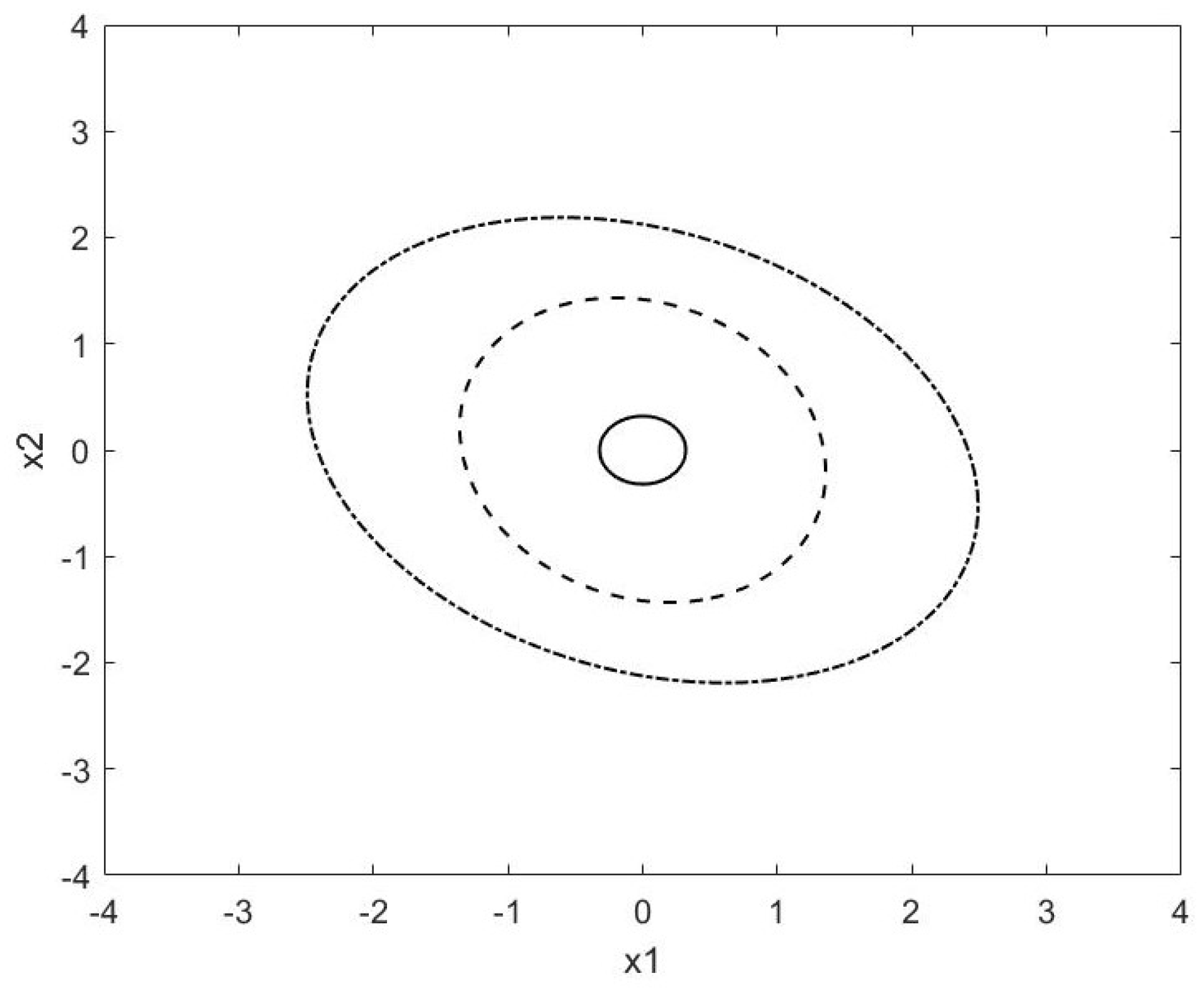
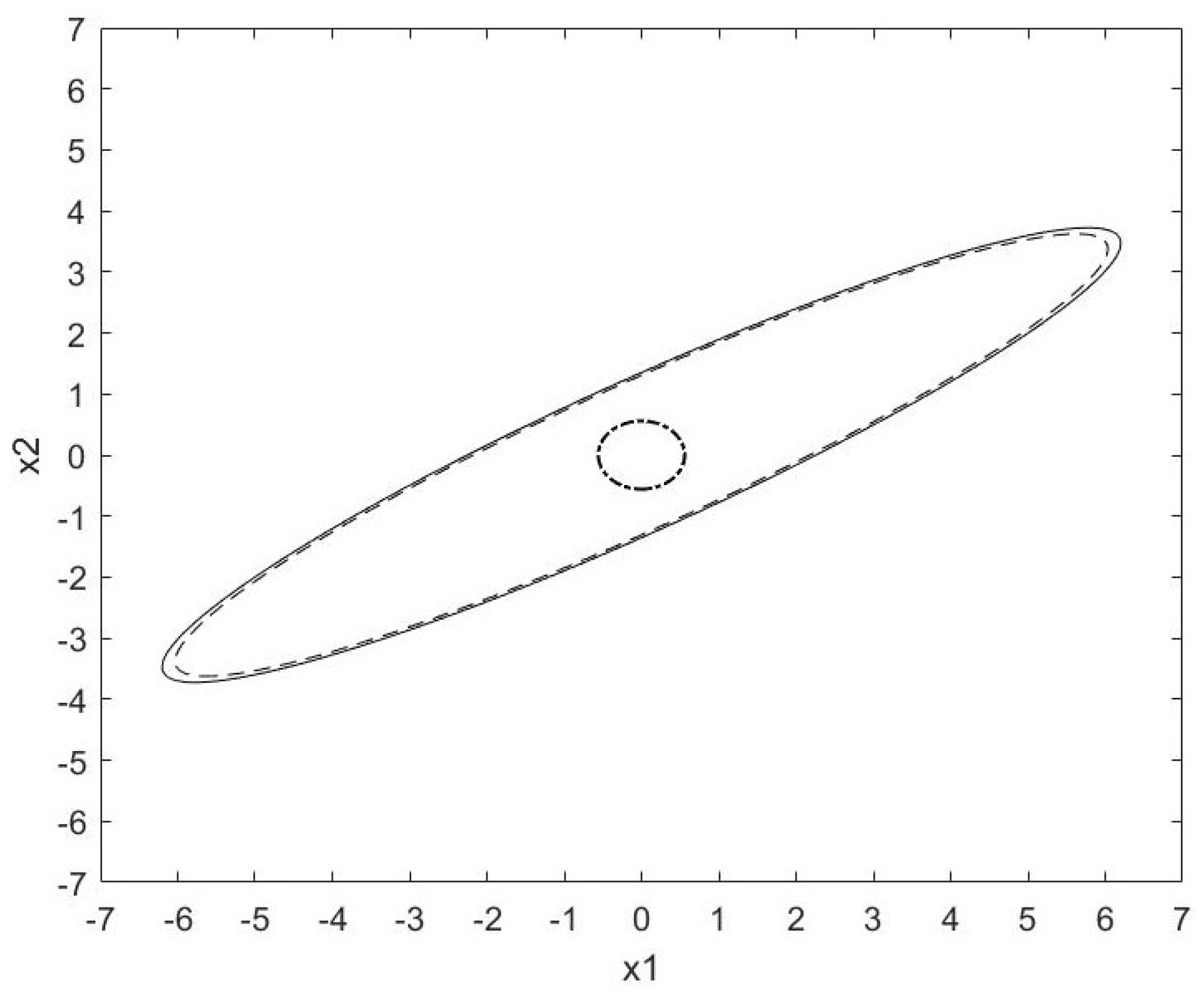
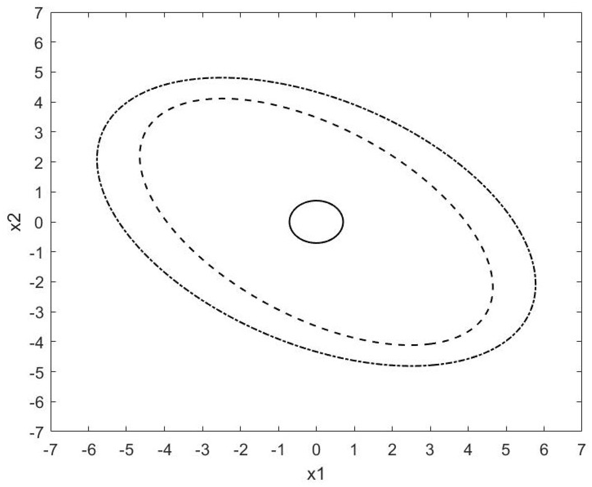
5. Numerical Examples

Example 1. 

(i) The robust control invariant set by Theorem 2

Consider a 2-dimensional linear system

$$\begin{array}{c}\hfill x\left(k+1\right)=Ax\left(k\right)+Bu\left(k\right)+B_{w}w\left(k\right)\end{array}$$

(15)

with the following parameters:

$$A=\left[\begin{array}{cc}2& 0.7\\ 2.7& 0.6\end{array}\right],B=\left[\begin{array}{c}2\\ 3\end{array}\right],B_w=\left[\begin{array}{c}0\\ 1\end{array}\right].$$

The disturbance $w\in W\subset R^1$, where

$$\begin{array}{c}\hfill W=\left\{w\in R^1\mid -0.1\le w\le 0.1\right\}.\end{array}$$

From the solutions P satisfying (7), the following are obtained:

$$\begin{array}{cc}\hfill & Q=\left[\begin{array}{cc}6.2030& -1.3219\\ -1.3219& 4.7953\end{array}\right],\hfill \\ \hfill & M=\left[\begin{array}{cc}-5.4379& 0.0654\end{array}\right].\hfill \end{array}$$

According to the substitutions of variables,

$$\begin{array}{cc}\hfill & P=Q^{-1}=\left[\begin{array}{cc}0.1713& 0.0472\\ 0.0472& 0.2216\end{array}\right],\hfill \\ \hfill & K=MP=\left[\begin{array}{cc}-0.9283& -0.2423\end{array}\right].\hfill \end{array}$$

Here, we take $\beta =0.9$, $\alpha =0.9$, and $\mu =10$. Therefore, the robustly controlled invariant set of the system (15) is

$$\begin{array}{c}\hfill {\Omega }_0=\left\{x\in R^n\mid x^T\left[\begin{array}{cc}0.1713& 0.0472\\ 0.0472& 0.2216\end{array}\right]x\le 1\right\}.\end{array}$$

The corresponding linear control law is $u=\left[\begin{array}{cc}-0.9283& -0.2423\end{array}\right]x$. The robustly controlled invariant set yielded from Theorem 2 is shown by the dashed-dotted ellipsoid in Figure 1.

(ii) The maximal robustly controlled invariant set by Theorem 3

Consider the 2-dimensional linear system in (15) with the same $A,B,B_{\omega }$, and disturbance, the maximal robustly controlled invariant set of the system (15) with a linear control law of $u=Kx$ can be obtained by solving the following optimization problem

$$\begin{array}{cc}\hfill & \underset{Q,M,\beta ,\mu }{max}{\left(detQ\right)}^{{\displaystyle \frac{1}{n}}}\hfill \\ \hfill & s.t\left[\begin{array}{ccc}-Q& AQ+BM& B_{\omega }\\ \ast & -\left(1-\beta \right)Q& 0\\ \ast & \ast & -\mu I\end{array}\right]⪯0.\hfill \end{array}$$

The solutions are obtained as follows:

$$\begin{array}{cc}\hfill & Q=\left[\begin{array}{cc}1.8464& -0.2841\\ -0.2841& 2.0533\end{array}\right],\hfill \\ \hfill & M=\left[\begin{array}{cc}-1.6438& -0.2337\end{array}\right].\hfill \end{array}$$

According to the changes of variables,

$$\begin{array}{cc}\hfill & P=Q^{-1}=\left[\begin{array}{cc}0.5534& 0.0766\\ 0.0766& 0.4976\end{array}\right],\hfill \\ \hfill & K=MP=\left[\begin{array}{cc}-0.9276& -0.2422\end{array}\right].\hfill \end{array}$$

If we set $\beta =0.9$ and $\alpha =0.99$, then $\mu =1$. Therefore, the robust control invariant set of the system (16) is

$$\begin{array}{c}\hfill {\Omega }_0=\left\{x\in R^n\mid x^T\left[\begin{array}{cc}0.5534& 0.0766\\ 0.0766& 0.4976\end{array}\right]x\le 1\right\}.\end{array}$$

The corresponding linear control law is $u=\left[\begin{array}{cc}-0.9276& -0.2422\end{array}\right]x$. The maximal robustly controlled invariant set yielded from Theorem 3 is shown by the dashed ellipsoid in Figure 1.

(iii) The robustly controlled invariant set by Theorem 4

Consider the 2-dimensional linear system in (15) and set $P=I$, the logarithmic norm of the system (15) with a linear control law of $u=Kx$ can be obtained by solving the following optimization problem:

$$\begin{array}{cc}\hfill & \underset{K,\lambda }{min}\lambda \hfill \\ \hfill & s.t2\lambda I-\left(A+BK\right)-{\left(A+BK\right)}^T⪰0.\hfill \end{array}$$

The obtained logarithmic norm and control gain are $\lambda =0.0308$ and $K=\left[\begin{array}{cc}-1.1354& -0.4493\end{array}\right]$, respectively. With the control gain $K=\left[\begin{array}{cc}-1.1354& -0.4493\end{array}\right]$, the robustly controlled invariant set is

$$\begin{array}{c}\hfill \Omega =\left\{x\in R^2\mid x^{T}x\le 0.1032\right\}.\end{array}$$

Remark 5. 

To reduce and limit the influence of disturbances on the system, the minimum robustly controlled invariant set needs to be considered. The robustly controlled invariant set yielded from Theorem 5 is represented by the solid ellipsoid in Figure 1. Examples 1–3 are the robustly controlled invariant sets corresponding to Theorems 2–4 under the same system. To reduce and limit the impact of disturbances on the system, we select the minimum robustly controlled invariant set. It can be seen from Figure 1 that Theorem 4 is the least conservative.

Example 2. 

(i) The robust control invariant set by Theorem 2

Consider a 2-dimensional linear system

$$\begin{array}{c}\hfill x\left(k+1\right)=Ax\left(k\right)+Bu\left(k\right)+B_{w}w\left(k\right)\end{array}$$

(16)

with the following parameters:

$$A=\left[\begin{array}{cc}-1.2& 3\\ -4& 5\end{array}\right],B=\left[\begin{array}{c}2\\ -4\end{array}\right],B_w=\left[\begin{array}{c}0\\ 2\end{array}\right].$$

The disturbance $w\in W\subset R^1$, where

$$\begin{array}{c}\hfill W=\left\{w\in R^1\mid -0.1\le w\le 0.1\right\}.\end{array}$$

From the solutions P satisfying (7), the following are obtained:

$$\begin{array}{cc}\hfill & Q=\left[\begin{array}{cc}38.3891& 21.4828\\ 21.4828& 13.8513\end{array}\right],\hfill \\ \hfill & M=\left[\begin{array}{cc}-11.0095& -5.0026\end{array}\right].\hfill \end{array}$$

According to the changes of variables,

$$\begin{array}{cc}\hfill & P=Q^{-1}=\left[\begin{array}{cc}0.1972& -0.3059\\ -0.3059& 0.5466\end{array}\right],\hfill \\ \hfill & K=MP=\left[\begin{array}{cc}-0.6408& 0.6334\end{array}\right].\hfill \end{array}$$

Here, we take $\beta =0.05$, $\alpha =0.5$, and $\mu =50$. Therefore, the robustly controlled invariant set of the system (16) is

$$\begin{array}{c}\hfill {\Omega }_0=\left\{x\in R^n\mid x^T\left[\begin{array}{cc}0.1972& -0.3059\\ -0.3059& 0.5466\end{array}\right]x\le 1\right\}.\end{array}$$

The corresponding linear control law is $u=\left[\begin{array}{cc}-0.6408& 0.6334\end{array}\right]x$. The robustly controlled invariant set yielded from Theorem 2 is shown by the solid ellipsoid in Figure 2.

(ii) The robustly controlled invariant set by Theorem 3

Considering the 2-dimensional linear system (16) with a linear control law of $u=Kx$, a solution can be obtained by solving the following optimization problem

$$\begin{array}{cc}\hfill & \underset{Q,M,\beta ,\mu }{max}{\left(detQ\right)}^{{\displaystyle \frac{1}{n}}}\hfill \\ \hfill & s.t.\left[\begin{array}{ccc}-Q& AQ+BM& B_{\omega }\\ \ast & -\left(1-\beta \right)Q& 0\\ \ast & \ast & -\mu I\end{array}\right]⪯0.\hfill \end{array}$$

The solutions are obtained as follows:

$$\begin{array}{cc}\hfill & Q=\left[\begin{array}{cc}36.4057& 20.3923\\ 20.3923& 13.1329\end{array}\right],\hfill \\ \hfill & M=\left[\begin{array}{cc}-10.4282& -4.7588\end{array}\right].\hfill \end{array}$$

According to the substitutions of variables,

$$\begin{array}{cc}\hfill & P=Q^{-1}=\left[\begin{array}{cc}0.2109& -0.3275\\ -0.3275& 0.5847\end{array}\right],\hfill \\ \hfill & K=MP=\left[\begin{array}{cc}-0.6408& 0.6328\end{array}\right].\hfill \end{array}$$

If we set $\beta =0.1$ and $\alpha =0.5$, then $\mu =50$. Therefore, the robustly controlled invariant set of the system (16) is

$$\begin{array}{c}\hfill {\Omega }_0=\left\{x\in R^n\mid x^T\left[\begin{array}{cc}0.2109& -0.3275\\ -0.3275& 0.5847\end{array}\right]x\le 1\right\}.\end{array}$$

The corresponding linear control law is $u=\left[\begin{array}{cc}-0.6408& 0.6328\end{array}\right]x$. The maximal robustly controlled invariant set yielded from Theorem 3 is shown by the dashed ellipsoid in Figure 2.

(iii) The robustly controlled invariant set by Theorem 4

Consider the 2-dimensional linear system (16) and set $P=I$. The logarithmic norm of the system (16) with a linear control law of $u=Kx$ can be obtained by solving the following optimization problem

$$\begin{array}{cc}\hfill & \underset{K,\lambda }{min}\lambda \hfill \\ \hfill & s.t.2\lambda I-\left(A+BK\right)-{\left(A+BK\right)}^T⪰0.\hfill \end{array}$$

The obtained logarithmic norm and control gain are $\lambda =-0.3600$ and $K=\left[\begin{array}{cc}0.3764& 1.4271\end{array}\right]$, respectively. With the control gain $K=\left[\begin{array}{cc}0.3764& 1.4271\end{array}\right]$, the robustly controlled invariant set is

$$\begin{array}{c}\hfill \Omega =\left\{x\in R^2\mid x^{T}x\le 0.3125\right\}.\end{array}$$

Remark 6. 

The robustly controlled invariant set yielded from Theorem 5 is represented by the dashed-dotted ellipsoid in Figure 2. It can be clearly seen from Figure 2 that the robust control invariant set obtained by the logarithmic norm method is the smallest and less conservative.

Example 3. 

(i) The robustly controlled invariant set by Theorem 3

Consider a 2-dimensional linear system

$$\begin{array}{c}\hfill x\left(k+1\right)=Ax\left(k\right)+Bu\left(k\right)+B_{w}w\left(k\right)\end{array}$$

(17)

with following parameters:

$$A=\left[\begin{array}{cc}4& 1.5\\ 5& 1\end{array}\right],B=\left[\begin{array}{c}1\\ 2\end{array}\right],B_w=\left[\begin{array}{c}0\\ 1\end{array}\right].$$

The disturbance $w\in W\subset R^1$, where

$$\begin{array}{c}\hfill W=\left\{w\in R^1\mid -0.1\le w\le 0.1\right\}.\end{array}$$

From the solutions P satisfying (7), the following are obtained:

$$\begin{array}{cc}\hfill & Q=\left[\begin{array}{cc}43.4286& -31.4263\\ -31.4263& 60.3967\end{array}\right],\hfill \\ \hfill & M=\left[\begin{array}{cc}-104.6118& 43.5510\end{array}\right].\hfill \end{array}$$

According to the substitutions of variables,

$$\begin{array}{cc}\hfill & P=Q^{-1}=\left[\begin{array}{cc}0.0369& 0.0192\\ 0.0192& 0.0266\end{array}\right],\hfill \\ \hfill & K=MP=\left[\begin{array}{cc}-3.0240& -0.8501\end{array}\right].\hfill \end{array}$$

Here, we take $\beta =0.1$, $\alpha =0.1$, and $\mu =90$. Therefore, the robustly controlled invariant set of the system (17) is

$$\begin{array}{c}\hfill {\Omega }_0=\left\{x\in R^n\mid x^T\left[\begin{array}{cc}0.0369& 0.0192\\ 0.0192& 0.0266\end{array}\right]x\le 1\right\}.\end{array}$$

The corresponding linear control law is $u=\left[\begin{array}{cc}-3.0240& -0.8501\end{array}\right]x$. The robustly controlled invariant set yielded of the Theorem 2 is shown by the dashed-dotted ellipsoid in Figure 3.

(ii) The robustly controlled invariant set by Theorem 3

Consider the 2-dimensional linear system in (17). The robustly controlled invariant set of the system (17) with a linear control law of $u=Kx$ can be obtained by solving the following optimization problem:

$$\begin{array}{cc}\hfill & \underset{Q,M,\beta ,\mu }{max}{\left(detQ\right)}^{{\displaystyle \frac{1}{n}}}\hfill \\ \hfill & s.t.\left[\begin{array}{ccc}-Q& AQ+BM& B_{\omega }\\ \ast & -\left(1-\beta \right)Q& 0\\ \ast & \ast & -\mu I\end{array}\right]⪯0.\hfill \end{array}$$

The solutions are obtained as follows:

$$\begin{array}{cc}\hfill & Q=\left[\begin{array}{cc}35.7873& -33.7164\\ -33.7164& 56.0413\end{array}\right],\hfill \\ \hfill & M=\left[\begin{array}{cc}-80.2426& 54.3734\end{array}\right].\hfill \end{array}$$

According to the substitutions of variables,

$$\begin{array}{cc}\hfill & P=Q^{-1}=\left[\begin{array}{cc}0.0645& 0.0388\\ 0.0388& 0.0412\end{array}\right],\hfill \\ \hfill & K=MP=\left[\begin{array}{cc}-3.0660& -0.8732\end{array}\right].\hfill \end{array}$$

If we set $\beta =0.5$ and $\alpha =0.5$, then $\mu =50$. Therefore, the robustly controlled invariant set of the system (17) is

$$\begin{array}{c}\hfill {\Omega }_0=\left\{x\in R^n\mid x^T\left[\begin{array}{cc}0.0645& 0.0388\\ 0.0388& 0.0412\end{array}\right]x\le 1\right\}.\end{array}$$

The corresponding linear control law is $u=\left[\begin{array}{cc}-3.0660& -0.8732\end{array}\right]x$. The robustly controlled invariant set yielded of the Theorem 3 is shown by the dashed ellipsoid in Figure 3.

(iii) The robustly controlled invariant set by Theorem 4

Consider the 2-dimensional linear system (17) and set $P=I$. The logarithmic norm of the system (17) with a linear control law of $u=Kx$ can be obtained by solving the following optimization problem:

$$\begin{array}{cc}\hfill & \underset{K,\lambda }{min}\lambda \hfill \\ \hfill & s.t.2\lambda I-\left(A+BK\right)-{\left(A+BK\right)}^T⪰0.\hfill \end{array}$$

The obtained logarithmic norm and control gain are $\lambda =0.8000$ and $K=\left[\begin{array}{cc}-3.2871& -0.2742\end{array}\right]$, respectively. With the control gain $K=\left[\begin{array}{cc}-3.2871& -0.2742\end{array}\right]$, the robustly controlled invariant set is

$$\begin{array}{c}\hfill \Omega =\left\{x\in R^2\mid x^{T}x\le 0.5\right\}.\end{array}$$

Remark 7. 

The robustly controlled invariant set yielded from Theorem 4 is represented by the solid ellipsoid in Figure 3. It can be seen from Figure 3 that the volume of the robustly controlled invariant set obtained in Example 3 is the smallest, so Theorem 4 is the least conservative.

6. Conclusions

In this paper, the sufficient condition for computing the robust control invariant set of linear discrete-time systems with additive bounded disturbances is discussed. The robust control invariant set is proposed by using two methods, difference inequality and LMI based on logarithmic norm, and solved by LMI optimization problem. In addition, we presented the computing method of a maximum and minimum robust control invariant set based on the above two methods. Results presented in this paper provide a new alternative method for computing the robust control invariant set and generalize the results of the robust control invariant set for discrete-time linear systems.

References

1. Rakovic, S.V.; Baric, M. Parameterized robust control invariant sets for linear systems: Theoretical advances and computational remarks. IEEE Trans. Autom. Control 2010, 55, 1599–1614. [Google Scholar] [CrossRef]
2. Tahir, F.; Jaimoukha, I.M. Robust Positively Invariant Sets for Linear Systems Subject to Model-Uncertainty and Disturbances. Ifac Proc. Vol. 2012, 45, 213–217. [Google Scholar] [CrossRef]
3. Raković, S.V.; Kerrigan, E.C.; Mayne, D.Q.; Kouramas, K.I. Optimized robust control invariance for linear discrete-time systems: Theoretical foundations. Automatica 2007, 43, 831–841. [Google Scholar] [CrossRef]
4. Tarraf, D.C.; Bauso, D. Finite alphabet control of logistic networks with discrete uncertainty. Syst. Control. Lett. 2014, 64, 20–26. [Google Scholar] [CrossRef]
5. Blanchini, F. Set invariance in control. Automatica 1999, 35, 1747–1767. [Google Scholar] [CrossRef]
6. Fiacchini, M.; Alamo, T.; Camacho, E.F. On the computation of convex robust control invariant sets for nonlinear systems. Automatica 2010, 46, 1334–1338. [Google Scholar] [CrossRef]
7. Blanchini, F.; Miani, S. Set-Theoretic Methods in Control; Birkhäuser: Boston, MA, USA, 2008; Volume 78. [Google Scholar]
8. Li, H.; Xie, L.; Wang, Y. On robust control invariance of Boolean control networks. Automatica 2016, 68, 392–396. [Google Scholar] [CrossRef]
9. Parise, F.; Valcher, M.E.; Lygeros, J. On the reachable set of the controlled gene expression system. In Proceedings of the 53rd IEEE Conference on Decision and Control, Los Angeles, CA, USA, 15–17 December 2014; pp. 4597–4604. [Google Scholar]
10. Rungger, M.; Tabuada, P. Computing Robust Controlled Invariant Sets of Linear Systems. IEEE Trans. Autom. Control 2017, 62, 3665–3670. [Google Scholar] [CrossRef]
11. Dorea, C.E.T.; Hennet, J.C. On Robust Positive Invariance of Unbounded Polyhedra. Ifac Proc. Vol. 1995, 28, 231–236. [Google Scholar] [CrossRef]
12. Rakovic, S.V.; Kerrigan, E.C.; Kouramas, K.I.; Mayne, D.Q. Invariant approximations of the minimal robust positively invariant set. IEEE Trans. Autom. Control 2005, 50, 406–410. [Google Scholar] [CrossRef] [Green Version]
13. Tahir, F.; Jaimoukha, I.M. Low-Complexity Polytopic Invariant Sets for Linear Systems Subject to Norm-Bounded Uncertainty. IEEE Trans. Autom. Control 2014, 60, 1416–1421. [Google Scholar] [CrossRef] [Green Version]
14. Lei, Y.; Yang, H. Dual optimization approach to set invariance conditions for discrete-time dynamic systems. Optim. Eng. 2023, 1–18. [Google Scholar] [CrossRef]
15. Si, X.; Yang, H. Constrained regulation problem for continuous-time stochastic systems under state and control constraints. J. Vib. Control 2022, 28, 3218–3230. [Google Scholar] [CrossRef]
16. Yu, S.; Zhou, Y.; Qu, T.; Xu, F.; Ma, Y. Control invariant sets of linear systems with bounded disturbances. Int. J. Control. Autom. Syst. 2018, 16, 622–629. [Google Scholar] [CrossRef]
17. Hewing, L.; Carron, A.; Wabersich, K.P.; Zeilinger, M.N. On a correspondence between probabilistic and robust invariant sets for linear systems. In Proceedings of the 2018 European Control Conference (ECC), Limassol, Cyprus, 12–15 June 2018. [Google Scholar]
18. Gao, D.; Li, Q.; Wang, M.; Luo, J.; Li, J. Ellipsoidal approximations of the minimal robust positively invariant set. ISA Trans. 2023; in press. [Google Scholar] [CrossRef]
19. Chen, Y.; Peng, H.; Grizzle, J.; Ozay, N. Data-driven computation of minimal robust control invariant set. In Proceedings of the 2018 IEEE Conference on Decision and Control (CDC), Miami, FL, USA, 17–19 December 2018. [Google Scholar]
20. Boyd, S.; El Ghaoui, L.; Feron, E.; Balakishnan, V. Linear Matrix Inequalities in System and Control Theory; Society for Industrial and Applied Mathematics: Philadelphia, PA, USA, 1994. [Google Scholar]
21. That, N.D.; Nam, P.T.; Ha, Q.P. Reachable Set Bounding for Linear Discrete-Time Systems with Delays and Bounded Disturbances. J. Optim. Theory Appl. 2013, 157, 96–107. [Google Scholar] [CrossRef]
22. Shingin, H.; Ohta, Y. Optimal Invariant Sets for Discrete-Time Systems Approximation of the Reachable Sets for Bounded Inputs. Trans. Soc. Instrum. Control. Eng. 2004, 40, 842–848. [Google Scholar] [CrossRef] [Green Version]
23. Yu, L. Robust Control: Linear Matrix Inequality Approach; Tsinghua University: Beijing, China, 2002. [Google Scholar]
24. Harville, D.A. Matrix Algebra from a Statistician’S Perspective; Taylor & Francis: Abingdon, UK, 1998. [Google Scholar]
25. Hu, G.D.; Liu, M. The weighted logarithmic matrix norm and bounds of the matrix exponentia. Linear Algebra Its Appl. 2004, 390, 145–154. [Google Scholar] [CrossRef] [Green Version]
26. Ström, T. On logarithmic norms. Siam J. Numer. Ann. 1975, 12, 741–753. [Google Scholar] [CrossRef]
27. Martin, R.H., Jr. Logarithmic norms and projections applied to linear differential systems. J. Math. Anal. Appl. 1974, 45, 432–454. [Google Scholar] [CrossRef] [Green Version]
28. Ding, W.; Hou, Z.; Wei, Y. Tensor logarithmic norm and its applications. Numer. Linear Algebra Appl. 2016, 23, 989–1006. [Google Scholar] [CrossRef]
29. Yang, R.; Zhang, G.; Sun, L. Finite-time robust simultaneous stabilization of a set of nonlinear time-delay systems. Int. J. Robust Nonlinear Control 2020, 30, 1733–1753. [Google Scholar] [CrossRef]
30. Liu, X.; Liu, W.; Li, Y.; Zhuang, J. Finite-time H control of stochastic time-delay Markovian jump systems. J. Shandong Univ. Sci. Technol. 2022, 41, 75–84. [Google Scholar]
31. Drazin, P.G. Nonlinear Systems; Cambridge University Press: Cambridge, UK, 1992; Volume 10. [Google Scholar]
Figure 1. Robustly controlled invariant sets of the system.
Mathematics 11 03421 g001
Figure 2. Robustly controlled invariant sets of the system.
Mathematics 11 03421 g002
Figure 3. Robustly controlledinvariant sets of the system.
Mathematics 11 03421 g003
Disclaimer/Publisher’s Note: The statements, opinions and data contained in all publications are solely those of the individual author(s) and contributor(s) and not of MDPI and/or the editor(s). MDPI and/or the editor(s) disclaim responsibility for any injury to people or property resulting from any ideas, methods, instructions or products referred to in the content.