Variational Approach to Modeling of Curvilinear Thin Inclusions with Rough Boundaries in Elastic Bodies: Case of a Rod-Type Inclusion

Abstract

In the framework of 2D-elasticity, an equilibrium problem for an inhomogeneous body with a curvilinear inclusion located strictly inside the body is considered. The elastic properties of the inclusion are assumed to depend on a small positive parameter $\delta$ characterizing its width and are assumed to be proportional to ${\delta }^{-1}$. Moreover, it is supposed that the inclusion has a curvilinear rough boundary. Relying on the variational formulation of the equilibrium problem, we perform the asymptotic analysis, as $\delta$ tends to zero. As a result, a variational model of an elastic body containing a thin curvilinear rod is constructed. Numerical calculations give a relative error between the initial and limit problems depending on $\delta$.

1. Introduction

The present paper deals with an equilibrium problem for an inhomogeneous body with a curvilinear inclusion located strictly inside the elastic body. The elastic properties of the inclusion are assumed to depend on a small positive parameter $\delta$ characterizing its width. More precisely, the Lamé coefficients are proportional to ${\delta }^{-1}$. Furthermore, it is supposed that the inclusion has a perturbed curvilinear boundary. This means that the boundary of the inclusion is rough. The main purpose of this paper is to pass to the limit as $\delta$ tends to zero. As a result, a model of an elastic body containing a thin elastic curvilinear inclusion inside is constructed (in the considered case, this is a rod-type inclusion). To derive the limit problem, we use an approach based on a variational formulation of the equilibrium problem (see, e.g., [1,2,3]). It is worth noting that in our consideration, we take into account the three key features, which, in our opinion, were taken into account simultaneously earlier only in [1], in the case of a soft inclusion. Namely, these three features are that the inclusion is located strictly inside the body, the inclusion has a curvilinear boundary, and the boundary of the inclusion is rough.

Imperfect interface problems and problems of the coupling of different models of elasticity are of the greatest interest in the description of composite materials. In the present time, various types of thin inclusion problems were considered. Papers [4,5] investigated thin elastic inclusions such as the Euler–Bernoulli beam and the Timoshenko beam. Thin rigid inclusions were considered in [6,7,8,9,10]. Problems of thin elastic junctions between elastic bodies were studied in [11,12,13]. In all the mentioned works, as a rule, the main attention was paid to the study of the well-posedness of variational (weak) formulations of corresponding boundary value problems for equilibrium models but not the derivation of such models.

Currently, there is a huge number of papers devoted to the asymptotic analysis of linear and non-linear models of elasticity with the aim to derive different types of imperfect interfaces between elastic bodies. For example, in [14], a higher-order imperfect interface was studied by using complex variables and asymptotic analysis. In [15,16,17], interface models were derived for coupled thermoelasticity (see also [18,19,20,21] for modeling soft and hard interfaces in 2D- and 3D-elasticity).

One can notice that there are not so many papers devoted to studies of curvilinear interfaces with rough boundaries. In this line, we can only mention that the curvilinear interface problems were considered in [1,18,22], while in [1,23,24,25,26], the roughness of the inclusions was taken into account.

Moreover, we mention refs. [25,27,28,29], in which multi-scale asymptotic analysis and computation of static and dynamics problems in curvilinear coordinates was proposed.

The rest of the article is organized as follows. In Section 2, the equilibrium problem for an elastic body with a narrow inclusion depending on a small parameter $\delta >0$ is formulated. Then, in Section 3, we introduce the special coordinate transformations, which allow us further in Section 4 to reformulate the initial problem and decompose it in such a way that the new variational problem is defined in a fixed domain that is independent of $\delta$. Section 5 is devoted to the justification of the asymptotic procedure, as a result of which the limit problem is derived. The numerical examples of Section 6 confirm the accuracy of the passage to the limit, justified in Section 5.

2. Statement of the Initial Problem

Let $\mathsf{\Omega }\subset {\mathbb{R}}^2$ be a convex bounded domain with a Lipschitz boundary $\partial \mathsf{\Omega }$; ${\mathsf{\Gamma }}_N$ and ${\mathsf{\Gamma }}_D$ be the parts of $\partial \mathsf{\Omega }$ such that ${\overline{\mathsf{\Gamma }}}_N\cup {\overline{\mathsf{\Gamma }}}_D=\partial \mathsf{\Omega }$ and $\mathrm{meas}{\mathsf{\Gamma }}_D>0$; and I, $I_1$, and $I_2$ be the three intervals lying on the abscissa axis $O{y}_1$ such that ${\overline{I}}_1\subset I_2$, ${\overline{I}}_2\subset I$. Moreover, assume I is the intersection of the domain $\mathsf{\Omega }$ with $O{y}_1$-axis.

We introduce the functions $\phi \in C^{1,1}\left(\overline{I}\right)$, ${\psi }_{-},{\psi }_{+}\in C^{0,1}\left(\overline{I}\right)$ such that

• ${\psi }_{+}-{\psi }_{-}>0$ on $I_1$;
• ${\psi }_{+}-{\psi }_{-}=0$ on $I\setminus {\overline{I}}_1$;
• $\phi =0$ on $I\setminus {\overline{I}}_2$;
• The graph of the function $\phi$ is located strictly inside the domain $\mathsf{\Omega }$.

Let us fix a small parameter $\delta >0$ and put

$${\mathsf{\Omega }}_{\pm }=\{(x_1,x_2)\in \mathsf{\Omega }|\pm x_2>\pm \phi \left(x_1\right),x_1\in I\},$$

$${\mathsf{\Omega }}_m^{\delta }=\{(y_1,y_2)\in \mathsf{\Omega }|\phi \left(y_1\right)+\delta {\psi }_{-}\left(y_1\right)<y_2<\phi \left(y_1\right)+\delta {\psi }_{+}\left(y_1\right),y_1\in I_1\},$$

$$S_{\pm }^{\delta }=\{(y_1,y_2)\in \mathsf{\Omega }|y_2=\phi \left(y_1\right)+\delta {\psi }_{\pm }\left(y_1\right),y_1\in I_1\},$$

$${\mathsf{\Omega }}_e^{\delta }=\mathsf{\Omega }\setminus \overline{{\mathsf{\Omega }}_m^{\delta }},{\mathsf{\Omega }}_{\pm }^{\delta }={\mathsf{\Omega }}_e^{\delta }\cap {\mathsf{\Omega }}_{\pm }.$$

Note that, for all small-enough $\delta >0$, the domain ${\mathsf{\Omega }}_m^{\delta }$ lies strictly inside $\mathsf{\Omega }$.

In our consideration, the domain $\mathsf{\Omega }$ is an elastic inhomogeneous body, containing a narrow curvilinear strip ${\mathsf{\Omega }}_m^{\delta }$ with width of order $\delta$ and with a rough boundary ${\overline{S}}_{+}^{\delta }\cup {\overline{S}}_{-}^{\delta }$, where roughness is characterized by functions ${\psi }_{\pm }$ (see Figure 1).

By $C^{\delta }$, $C^0$, we denote the tensors characterizing the material constants of the inclusion ${\mathsf{\Omega }}_m^{\delta }$ and the elastic matrix ${\mathsf{\Omega }}_e^{\delta }$, respectively, with usual symmetrical and elliptical properties (see, e.g., [30]). We prescribe homogeneous Dirichlet’s conditions on ${\mathsf{\Gamma }}_D$ and Neumann’s conditions on the remaining part ${\mathsf{\Gamma }}_N$ of the external boundary $\partial \mathsf{\Omega }$. This means that the body $\mathsf{\Omega }$ is clamped on ${\mathsf{\Gamma }}_D$, whereas the force $\mathit{g}\in L_2\left({\mathsf{\Gamma }}_N\right)$ is applied to ${\mathsf{\Gamma }}_N$.

We formulate the equilibrium problem for the body $\mathsf{\Omega }$ with the inclusion ${\mathsf{\Omega }}_m^{\delta }$ in the framework of the two-dimensional elasticity. Let $\mathit{u}=(u_1,u_2)$ be a vector of displacements of the composite body and $\sigma \left(\mathit{u}\right)={\left({\sigma }_{ij}\left(\mathit{u}\right)\right)}_{i,j=1,2}$ and $\epsilon \left(\mathit{u}\right)={\left({\epsilon }_{ij}\left(\mathit{u}\right)\right)}_{i,j=1,2}$ be the stress and the strain tensors, respectively, where

$${\epsilon }_{ij}\left(\mathit{u}\right)=\frac{1}{2}(u_{i,j}+u_{j,i}),i,j=1,2,$$

$$\sigma \left(\mathit{u}\right)=\left\{\begin{array}{cc}{C}^0\epsilon \left(\mathit{u}\right)\hfill & \mathrm{in}{\mathsf{\Omega }}_e^{\delta },\hfill \\ C^{\delta }\epsilon \left(\mathit{u}\right)\stackrel{\mathrm{def}}{=}{\delta }^{-1}{C}^1\epsilon \left(\mathit{u}\right)={\delta }^{-1}\left({\lambda }_{m}Itr\epsilon \left(\mathit{u}\right)+2{\mu }_m\epsilon \left(\mathit{u}\right)\right)\hfill & \mathrm{in}{\mathsf{\Omega }}_m^{\delta }.\hfill \end{array}\right.$$

Here and further, lower indices after the comma denote the operation of differentiation with respect to the corresponding coordinate, the summation over repeated indices is performed, ${\lambda }_m$ and ${\lambda }_m$ are the Lamé coefficients such that ${\lambda }_m+2{\mu }_m>0$ and ${\mu }_m>0$; hence, the tensor $C^1$ is positive definite. In general, the elastic matrix characterized by the tensor $C^0$ is anisotropic and homogeneous with the elastic coefficients belonging to $L_{loc}^{\infty }\left({\mathbb{R}}^2\right)$.

The equilibrium problem under study is the following boundary value problem:

$$-{\sigma }_{ij,j}\left({\mathit{u}}_{\delta }\right)=0\mathrm{in}\mathsf{\Omega },i=1,2,$$

(1)

$${\mathit{u}}_{\delta }=0\mathrm{on}{\mathsf{\Gamma }}_D,$$

(2)

$${\sigma }_{ij}\left({\mathit{u}}_{\delta }\right)n_j=g_i\mathrm{on}{\mathsf{\Gamma }}_N,i=1,2,$$

(3)

where $\mathit{n}=(n_1,n_2)$ is a normal unit vector to $\partial \mathsf{\Omega }$, $\mathit{g}=(g_1,g_2)\in L_2{\left({\mathsf{\Gamma }}_N\right)}^2$ is a given traction.

In the sequel, the following variational (weak) formulation of Problems (1)–(3) is used: find a function ${\mathit{u}}_{\delta }\in H_{{\mathsf{\Gamma }}_D}\left(\mathsf{\Omega }\right)$ satisfying the variational equality

$$\underset{\mathsf{\Omega }}{\int }\sigma \left({\mathit{u}}_{\delta }\right):\epsilon \left(\mathit{v}\right)d\mathit{y}=\underset{{\mathsf{\Gamma }}_N}{\int }\mathit{g}\mathit{v}ds$$

(4)

for all kinematically admissible displacement test functions $\mathit{v}\in H_{{\mathsf{\Gamma }}_D}^1\left(\mathsf{\Omega }\right)$, where

$$H_{{\mathsf{\Gamma }}_D}\left(\mathsf{\Omega }\right)=\{\mathit{v}\in H^1{\left(\mathsf{\Omega }\right)}^2|\mathit{v}=0\mathrm{a}.\mathrm{e}.\mathrm{on}{\mathsf{\Gamma }}_D\}.$$

3. Transformations of Coordinates

Introduce into consideration the following sets:

$${\mathsf{\Omega }}_m=\{(z_1,z_2)\in {\mathbb{R}}^2|{\psi }_{-}\left(z_1\right)<z_2<{\psi }_{+}\left(z_1\right),z_1\in I_1\},$$

$$S_{\pm }=\{(z_1,z_2)\in {\mathbb{R}}^2|z_2={\psi }_{\pm }\left(z_1\right),z_1\in I_1\},$$

$$S=\{(x_1,x_2)\in {\mathbb{R}}^2|x_2=\phi \left(x_1\right),x_1\in I_1\},$$

which are independent of $\delta$, and define coordinate transformations mapping domains ${\mathsf{\Omega }}_{\pm }^{\delta }$ and ${\mathsf{\Omega }}_m^{\delta }$ onto domains ${\mathsf{\Omega }}_{\pm }$ and ${\mathsf{\Omega }}_m$, respectively. For this purpose, take two convex open domains $D_1$ and $D_2$ such that $I_2=D_2\cap O{y}_1$, ${\overline{I}}_1\subset D_1$, ${\overline{D}}_1\subset D_2$, ${\overline{D}}_2\subset \mathsf{\Omega }$, and consider the following domains:

$$D_i^{\phi }=\left\{(z_1,z_2)\right|z_1=y_1,z_2=\phi \left(y_1\right)+y_2,(y_1,y_2)\in D_i\},i=1,2.$$

The inclusions $\overline{S}\subset D_1^{\phi }$ and ${\overline{D}}_1^{\phi }\subset D_2^{\phi }$ hold. Additionally, assume that domain $D_2^{\phi }$ lies strictly inside $\mathsf{\Omega }$.

Further, consider a smooth cut-off function $\theta \in C^1\left(\overline{\mathsf{\Omega }}\right)$ such that

$$\theta =1\mathrm{in}{D}_1^{\phi };0<\theta <1\mathrm{in}{D}_2^{\phi };\theta =0\mathrm{in}\mathsf{\Omega }\setminus {\overline{D}}_2^{\phi }.$$

Finally, define the coordinate transformations $x={\mathsf{\Lambda }}_{\pm }\left(y\right)$ and $z={\mathsf{\Lambda }}_m\left(y\right)$ by the formulas

$$x_1=y_1,x_2=y_2-\delta {\psi }_{\pm }\left(y_1\right)\theta (y_1,y_2),(y_1,y_2)\in {\mathsf{\Omega }}_{\pm }^{\delta },(x_1,x_2)\in {\mathsf{\Omega }}_{\pm },$$

(5)

$$z_1=y_1,z_2=\frac{y_2-\phi \left(y_1\right)}{\delta },(y_1,y_2)\in {\mathsf{\Omega }}_m^{\delta },(z_1,z_2)\in {\mathsf{\Omega }}_m,$$

(6)

respectively. It is easy to see that Transformations (5) and (6) are one-to-one. Moreover, these coordinate transformations generate an isomorphism between $H^1\left({\mathsf{\Omega }}_{\pm }\right)$, $H^1\left({\mathsf{\Omega }}_m\right)$ and $H^1\left({\mathsf{\Omega }}_{\pm }^{\delta }\right)$, $H^1\left({\mathsf{\Omega }}_m^{\delta }\right)$, respectively (see, e.g., Chapter 2, Lemma 3.4 in [31]). By $\mathit{y}={\mathsf{\Lambda }}_{\pm }^{-1}\left(\mathit{x}\right)$ and $\mathit{y}={\mathsf{\Lambda }}_m^{-1}\left(\mathit{z}\right)$, we further denote the inverse transformations to (5) and (6), respectively.

4. Decomposition and Transformation of the Problem

Following the arguments from [1,2,32] with natural modifications, we now rewrite Problem (4) in the equivalent form. We introduce the set

$$\begin{array}{ll}{K}^{\delta }=& \{({\mathit{v}}^{+},{\mathit{v}}^{-},{\mathit{v}}^m)\in H^1\left({\mathsf{\Omega }}_{+}^{\delta }\right)\times H^1\left({\mathsf{\Omega }}_{-}^{\delta }\right)\times H^1\left({\mathsf{\Omega }}_m^{\delta }\right)|\\ & {\mathit{v}}^{\pm }=0\mathrm{a}.\mathrm{e}.\mathrm{on}{\mathsf{\Gamma }}_D\cap \partial {\mathsf{\Omega }}_{\pm }^{\delta },{\mathit{v}}^{\pm }={\mathit{v}}^m\mathrm{a}.\mathrm{e}.\mathrm{on}{S}_{\pm }^{\delta },{\mathit{v}}^{+}={\mathit{v}}^{-}\mathrm{a}.\mathrm{e}.\mathrm{on}\partial {\mathsf{\Omega }}_{-}^{\delta }\cap \partial {\mathsf{\Omega }}_{+}^{\delta }\},\hfill \end{array}$$

and define a variational problem: find a triplet $({\mathit{u}}_{\delta }^{+},{\mathit{u}}_{\delta }^{-},{\mathit{u}}_{\delta }^m)\in K^{\delta }$ satisfying the equality

$$\begin{array}{cc}\hfill \underset{{\mathsf{\Omega }}_{+}^{\delta }}{\int }{C}^0\epsilon \left({\mathit{u}}_{\delta }^{+}\right):\epsilon \left({\mathit{v}}^{+}\right)& d\mathit{y}+\underset{{\mathsf{\Omega }}_{-}^{\delta }}{\int }{C}^0\epsilon \left({\mathit{u}}_{\delta }^{-}\right):\epsilon \left({\mathit{v}}^{-}\right)d\mathit{y}\hfill \\ & +\frac{1}{\delta }\underset{{\mathsf{\Omega }}_m^{\delta }}{\int }{C}^1\epsilon \left({\mathit{u}}_{\delta }^m\right):\epsilon \left({\mathit{v}}^m\right)d\mathit{y}=\underset{{\mathsf{\Gamma }}_N\cap \partial {\mathsf{\Omega }}_{+}^{\delta }}{\int }\mathit{g}{\mathit{v}}^{+}ds+\underset{{\mathsf{\Gamma }}_N\cap \partial {\mathsf{\Omega }}_{-}^{\delta }}{\int }\mathit{g}{\mathit{v}}^{-}ds\hfill \end{array}$$

(7)

for all $({\mathit{v}}^{+},{\mathit{v}}^{-},{\mathit{v}}^m)\in K^{\delta }.$

Clearly, Problem (7) has a unique solution $({\mathit{u}}_{\delta }^{+},{\mathit{u}}_{\delta }^{-},{\mathit{u}}_{\delta }^m)$ for all $\delta >0$. Moreover, the relation

$${\mathit{u}}_{\delta }=\left\{\begin{array}{c}{\mathit{u}}_{\delta }^{\pm }\mathrm{a}.\mathrm{e}.\mathrm{in}{\mathsf{\Omega }}_{\pm }^{\delta },\hfill \\ {\mathit{u}}_{\delta }^m\mathrm{a}.\mathrm{e}.\mathrm{in}{\mathsf{\Omega }}_m^{\delta }\hfill \end{array}\right.$$

holds, where ${\mathit{u}}_{\delta }$ is the solution to Problem (4).

Let $K\subset H^1\left({\mathsf{\Omega }}_{-}\right)\times H^1\left({\mathsf{\Omega }}_{+}\right)\times H^1\left({\mathsf{\Omega }}_m\right)$ be the image of the set $K^{\delta }$ under the coordinate transformations (5) and (6),

$$\begin{array}{cc}\hfill K=& \left\{\right({\mathit{v}}^{+},{\mathit{v}}^{-},{\mathit{v}}^m)\in H^1\left({\mathsf{\Omega }}_{+}\right)\times H^1\left({\mathsf{\Omega }}_{-}\right)\times H^1\left({\mathsf{\Omega }}_m\right)|\hfill \\ & \hspace{1em}{\mathit{v}}^{\pm }{{|}_S={\mathit{v}}^m|}_{S_{\pm }},{\mathit{v}}^{\pm }=0\mathrm{a}.\mathrm{e}.\mathrm{on}{\mathsf{\Gamma }}_D\cap \partial {\mathsf{\Omega }}_{\pm },{\mathit{v}}^{+}={\mathit{v}}^{-}\mathrm{a}.\mathrm{e}.\mathrm{on}(\partial {\mathsf{\Omega }}_{-}\cap \partial {\mathsf{\Omega }}_{+})\setminus \overline{S}\}.\hfill \end{array}$$

The equality ${\mathit{v}}^{\pm }{{|}_S={\mathit{v}}^m|}_{S_{\pm }}$ in the definition of K means that

$${\mathit{v}}^{\pm }(x_1,\phi \left(x_1\right))={\mathit{v}}^m(x_1,{\psi }_{\pm }\left(x_1\right))\mathrm{for} \mathrm{all}{x}_1\in I_1.$$

(8)

After applying coordinate transformations $\mathit{y}={\mathsf{\Lambda }}_{\pm }^{-1}\left(\mathit{x}\right)$ and $\mathit{y}={\mathsf{\Lambda }}_m^{-1}\left(\mathit{z}\right)$ to the variational equality (7), we conclude that the transformed displacements

$${\tilde{\mathit{u}}}_{\delta }^{\pm }\left(\mathit{x}\right)={\mathit{u}}_{\delta }^{\pm }\left({\mathsf{\Lambda }}_{\pm }^{-1}\left(\mathit{x}\right)\right),{\tilde{\mathit{u}}}_{\delta }^m\left(\mathit{z}\right)={\mathit{u}}_{\delta }^m\left({\mathsf{\Lambda }}_m^{-1}\left(\mathit{z}\right)\right)$$

satisfy the variational equality

$$\begin{array}{c}{A}_{+}^{\delta }({\tilde{\mathit{u}}}_{\delta }^{+},{\mathit{v}}^{+})+A_{-}^{\delta }({\tilde{\mathit{u}}}_{\delta }^{-},{\mathit{v}}^{-})\hfill \\ \hspace{1em}\hspace{1em}\hspace{1em}\hspace{1em}\hspace{1em}\hspace{1em}\hspace{1em}\hspace{1em}+\underset{{\mathsf{\Omega }}_m}{\int }{C}^1{e}^{\delta }\left({\tilde{\mathit{u}}}_{\delta }^m\right):e^{\delta }\left({\mathit{v}}^m\right)d\mathit{z}=\underset{\partial {\mathsf{\Omega }}^{+}\cap {\mathsf{\Gamma }}_N}{\int }\mathit{g}{\mathit{v}}^{+}ds+\underset{\partial {\mathsf{\Omega }}^{-}\cap {\mathsf{\Gamma }}_N}{\int }\mathit{g}{\mathit{v}}^{-}ds\hfill \end{array}$$

(9)

for any triplet $({\mathit{v}}^{+},{\mathit{v}}^{-},{\mathit{v}}^m)\in K$, where

$$A_{\pm }^{\delta }({\mathit{u}}^{\pm },{\mathit{v}}^{\pm })=\underset{{\mathsf{\Omega }}_{\pm }}{\int }{J}_{\delta }^{\pm }{C}^{0}E({\mathsf{\Psi }}_{\delta }^{\pm };{\mathit{u}}^{\pm }):E({\mathsf{\Psi }}_{\delta }^{\pm };{\mathit{v}}^{\pm })d\mathit{x},$$

$$E_{ij}({\mathsf{\Psi }}_{\delta }^{\pm };\mathit{v})=(1/2)\left(v_{i,k}{\left({\mathsf{\Psi }}_{\delta }^{\pm }\right)}_{kj}+v_{j,k}{\left({\mathsf{\Psi }}_{\delta }^{\pm }\right)}_{ki}\right),i,j=1,2;$$

$$e^{\delta }\left({\mathit{v}}^m\right)=\left(\begin{array}{cc}{v}_{1,1}^m-\frac{{\phi }^{\prime }}{\delta }{v}_{1,2}^m& \frac{1}{2}\left(\frac{1}{\delta }{v}_{1,2}^m+v_{2,1}^m-\frac{{\phi }^{\prime }}{\delta }{v}_{2,2}^m\right)\\ \frac{1}{2}\left(\frac{1}{\delta }{v}_{1,2}^m+v_{2,1}^m-\frac{{\phi }^{\prime }}{\delta }{v}_{2,2}^m\right)& \frac{1}{\delta }{v}_{2,2}^m\end{array}\right),$$

with the Jacobi matrices ${\mathsf{\Psi }}_{\delta }^{\pm }$ and the Jacobian $J_{\delta }^{\pm }$ of the transformations $\mathit{y}={\mathsf{\Lambda }}_{\pm }^{-1}\left(\mathit{x}\right)$.

In the sequel, we use the first-order asymptotic expansions (see, e.g., [33,34])

$$A_{\pm }^{\delta }(\mathit{u},\mathit{v})=A_{\pm }(\mathit{u},\mathit{v})+\delta r_{\pm }(\delta ,\mathit{u},\mathit{v}),A_{\pm }(\mathit{u},\mathit{v})=\underset{{\mathsf{\Omega }}_{\pm }}{\int }{C}^0\epsilon \left(\mathit{u}\right):\epsilon \left(\mathit{v}\right)d\mathit{x},$$

(10)

where

$$|r_{\pm }{(\delta ,\mathit{u},\mathit{v})|\le c(\parallel \mathit{u}\parallel }_{H^1\left({\mathsf{\Omega }}_{\pm }\right)}^2+{\parallel \mathit{v}\parallel }_{H^1\left({\mathsf{\Omega }}_{\pm }\right)}^2),$$

(11)

with a constant c independent of $\delta$, $\mathit{u}$, and $\mathit{v}$.

5. Justification of the Asymptotic Analysis

It is well-known that uniform estimates play an essential role in asymptotic analysis (see, e.g., [20,35,36,37]. Here, we formulate and prove some Korn-type estimates. Primarily, we recall the following Lemmas 1 and 2.

Lemma 1

([2]). For any function $v\in H^1\left({\mathsf{\Omega }}_m\right)$ the following inequality holds:

$${\parallel v\parallel }_{L_2\left({\mathsf{\Omega }}_m\right)}^2\le c\left({\parallel v_{,2}\parallel }_{L_2\left({\mathsf{\Omega }}_m\right)}^2+{\parallel v\parallel }_{L_2\left(S_{\alpha }\right)}^2\right),\alpha \in \{-,+\},$$

with a constant c independent of v.

Lemma 2

([1]). For all small-enough $\delta >0$ and any triplet $({\mathit{v}}^{+},{\mathit{v}}^{-},{\mathit{v}}^m)\in K$ the following inequality holds:

$$\begin{array}{l}c\left({\parallel {\mathit{v}}^{+}\parallel }_{H^1\left({\mathsf{\Omega }}_{+}\right)}^2+{\parallel {\mathit{v}}^{-}\parallel }_{H^1\left({\mathsf{\Omega }}_{-}\right)}^2\right.\\ \left.+\delta \parallel v_{1,1}^m-\frac{{\phi }^{\prime }}{\delta }{v}_{1,2}^m{\parallel }_{L_2\left({\mathsf{\Omega }}_m\right)}^2+\frac{1}{\delta }\parallel v_{1,2}^m{\parallel }_{L_2\left({\mathsf{\Omega }}_m\right)}^2+\delta \parallel v_{2,1}^m-\frac{{\phi }^{\prime }}{\delta }{v}_{2,2}^m{\parallel }_{L_2\left({\mathsf{\Omega }}_m\right)}^2+\frac{1}{\delta }{\parallel v_{2,2}^m\parallel }_{L_2({\mathsf{\Omega }}_m)}^2\right)\\ \hspace{1em}\hspace{1em}\hspace{1em}\hspace{1em}\hspace{1em}\hspace{1em}\hspace{1em}\le \underset{{\mathsf{\Omega }}_{+}}{\int }{C}^0\epsilon \left({\mathit{v}}^{+}\right):\epsilon \left({\mathit{v}}^{+}\right)d\mathit{x}+\underset{{\mathsf{\Omega }}_{-}}{\int }{C}^0\epsilon \left({\mathit{v}}^{-}\right):\epsilon \left({\mathit{v}}^{-}\right)d\mathit{x}\\ \hspace{1em}\hspace{1em}\hspace{1em}\hspace{1em}\hspace{1em}\hspace{1em}\hspace{1em}\hspace{1em}\hspace{1em}\hspace{1em}\hspace{1em}\hspace{1em}\hspace{1em}\hspace{1em}\hspace{1em}\hspace{1em}\hspace{1em}\hspace{1em}\hspace{1em}\hspace{1em}\hspace{1em}\hspace{1em} +\delta \underset{{\mathsf{\Omega }}_m}{\int }{C}^1{e}^{\delta }\left({\mathit{v}}^m\right):e^{\delta }\left({\mathit{v}}^m\right)d\mathit{z}\end{array}$$

with a constant c independent of δ and $({\mathit{v}}^{+},{\mathit{v}}^{-},{\mathit{v}}^m)$.

Lemmas 1 and 2 allow us to prove Theorems 1–3 that follow.

Theorems 1 and 2 are preparatory in nature.

Theorem 1.

The solution $({\tilde{\mathit{u}}}_{\delta }^{+},{\tilde{\mathit{u}}}_{\delta }^{-},{\tilde{\mathit{u}}}_{\delta }^m)$ of Problem (9) satisfies the following uniform in δ estimates:

$${\parallel {\tilde{\mathit{u}}}_{\delta }^{+}\parallel }_{H^1{\left({\mathsf{\Omega }}_{+}\right)}^2}\le c,{\parallel {\tilde{\mathit{u}}}_{\delta }^{-}\parallel }_{H^1{\left({\mathsf{\Omega }}_{-}\right)}^2}\le c,$$

(12)

$${\delta }^{-1}{\parallel {\tilde{u}}_{\delta 2,2}^m\parallel }_{L_2\left({\mathsf{\Omega }}_m\right)}\le c,$$

(13)

$$\parallel {\tilde{u}}_{\delta 1,1}^m-\frac{{\phi }^{\prime }}{\delta }{\tilde{u}}_{\delta 1,2}^m{\parallel }_{L_2\left({\mathsf{\Omega }}_m\right)}\le c,{\parallel {\tilde{u}}_{\delta 2,1}^m+\frac{{\tilde{u}}_{\delta 1,2}^m}{\delta }\parallel }_{L_2\left({\mathsf{\Omega }}_m\right)}\le c,$$

(14)

$${\delta }^{-\frac{1}{2}}{\parallel {\tilde{u}}_{\delta 1,2}^m\parallel }_{L_2\left({\mathsf{\Omega }}_m\right)}\le c.$$

(15)

Proof. 

Let us take $({\tilde{\mathit{u}}}_{\delta }^{+},{\tilde{\mathit{u}}}_{\delta }^{-},{\tilde{\mathit{u}}}_{\delta }^m)$ in (7) as the test functions and apply the coordinate transformations (5) and (6). Taking into account (10), (11), and Korn’s inequality in the domains ${\mathsf{\Omega }}_{\pm }$, we obtain (12)–(14). Estimate (15) follows directly from Lemma 2 and (12)–(14). □

Theorem 2.

There exists a sequence, still denoted by δ, and limit functions ${\mathit{u}}^{\pm }\in H^1\left({\mathsf{\Omega }}_{\pm }\right)$ and $p_i\in L_2\left({\mathsf{\Omega }}_m\right)$, $i=1,2,3$, such that the following limiting relations

$${\tilde{\mathit{u}}}_{\delta }^{\pm }\to {\mathit{u}}^{\pm }weakly in{H}^1{\left({\mathsf{\Omega }}_{\pm }\right)}^2,$$

$${\tilde{\mathit{u}}}_{\delta }^m\to {\mathit{u}}^{m}weakly in{L}_2{\left({\mathsf{\Omega }}_m\right)}^2,$$

$${\tilde{u}}_{\delta 1,1}^m-\frac{{\phi }^{\prime }}{\delta }{\tilde{u}}_{\delta 1,2}^m\to p_{1}weakly in{L}_2\left({\mathsf{\Omega }}_m\right),$$

$$\frac{{\tilde{u}}_{\delta 1,2}^m}{\delta }+{\tilde{u}}_{\delta 2,1}^m\to p_{2}weakly in{L}_2\left({\mathsf{\Omega }}_m\right),$$

$$\frac{{\tilde{u}}_{\delta 2,2}^m}{\delta }\to p_{3}weakly in{L}_2\left({\mathsf{\Omega }}_m\right),$$

$${\tilde{\mathit{u}}}_{\delta ,2}^m\to {\mathit{u}}_{,2}^m=0strongly in{L}_2{\left({\mathsf{\Omega }}_m\right)}^2.$$

(16)

$${\tilde{u}}_{\delta 1,1}^m+{\phi }^{\prime }{\tilde{u}}_{\delta 2,1}^m\to p_1+{\phi }^{\prime }{p}_{2}weakly in{L}_2\left({\mathsf{\Omega }}_m\right)$$

(17)

hold true as $\delta \to 0+$.

Proof. 

The first six limiting relations follow from Theorem 1 and the weak compactness property of bounded sets in the spaces $L_2\left({\mathsf{\Omega }}_m\right)$ and $H^1\left({\mathsf{\Omega }}_{\pm }\right)$.

Now, let us prove (17). For any function $\eta \in C_0^{\infty }\left({\mathsf{\Omega }}_m\right)$, we have

$$\underset{{\mathsf{\Omega }}_m}{\int }(p_1+{\phi }^{\prime }{p}_2)\eta d\mathit{z}=\underset{\delta \to 0}{lim}\underset{{\mathsf{\Omega }}_m}{\int }\left({\tilde{u}}_{\delta 1,1}^m-\frac{{\phi }^{\prime }}{\delta }{\tilde{u}}_{\delta 1,2}^m+{\phi }^{\prime }(\frac{{\tilde{u}}_{\delta 1,2}^m}{\delta }+{\tilde{u}}_{\delta 2,1}^m)\right)\eta d\mathit{z}$$

$$=\underset{\delta \to 0}{lim}\underset{{\mathsf{\Omega }}_m}{\int }\left({\tilde{u}}_{\delta 1,1}^m+{\phi }^{\prime }{\tilde{u}}_{\delta 2,1}^m\right)\eta d\mathit{z}=-\underset{\delta \to 0}{lim}\underset{{\mathsf{\Omega }}_m}{\int }\left({\tilde{u}}_{\delta 1}^m{\eta }_{,1}+{\tilde{u}}_{\delta 2}^m{\left({\phi }^{\prime }\eta \right)}_{,1}\right)d\mathit{z}$$

$$=-\underset{{\mathsf{\Omega }}_m}{\int }((u_1^m+{\phi }^{\prime }{u}_2^m){\eta }_{,1}+{\phi }^{″}\eta u_2)d\mathit{z},$$

which gives (17). Moreover, additionally the following equality holds true:

$$p_1+{\phi }^{\prime }{p}_2=u_{1,1}^m+{\phi }^{\prime }{u}_{2,1}^m\in L_2\left({\mathsf{\Omega }}_m\right).$$

(18)

□

Remark 1.

Note that, in general, functions $u_{1,1}^m$ and $u_{2,1}^m$ do not belong to the space $L_2\left({\mathsf{\Omega }}_m\right)$.

Remark 2.

Due to (16), the function ${\mathit{u}}^m$ does not depend on $z_2$. From this fact, it follows that the traces of functions ${\mathit{u}}^{+}$ and ${\mathit{u}}^{-}$ on S coincide with each other.

Theorem 3 is the main result of this paper.

Theorem 3.

Let $({\tilde{\mathit{u}}}_{\delta }^{+},{\tilde{\mathit{u}}}_{\delta }^{-},{\tilde{\mathit{u}}}_{\delta }^m)\in K$ be a solution of Problem (9) and $({\mathit{u}}^{+},{\mathit{u}}^{-})$ be a solution of the following variational problem: find $\mathit{u}=({\mathit{u}}^{+},{\mathit{u}}^{-})$ satisfying the variational equality

$$\underset{\mathsf{\Omega }}{\int }{C}^0\epsilon \left(\mathit{u}\right):\epsilon \left(\mathit{v}\right)d\mathit{x}+\underset{S}{\int }\frac{4{\mu }_m({\lambda }_m+{\mu }_m)({\psi }_{+}-{\psi }_{-})}{({\lambda }_m+2{\mu }_m){(1+{{\phi }^{\prime }}^2)}^{\frac{1}{2}}}({\mathit{\tau }}^t\nabla \mathit{u}\mathit{\tau })({\mathit{\tau }}^t\nabla \mathit{v}\mathit{\tau })ds=\underset{{\mathsf{\Gamma }}_N}{\int }\mathit{g}\mathit{v}ds$$

(19)

for all $\mathit{v}\in K_l$, where ${\mathit{u}}^{\pm }{=\mathit{u}|}_{{\mathsf{\Omega }}_{\pm }}$ are the restrictions of $\mathit{u}$ on ${\mathsf{\Omega }}_{\pm }$,

$$K_l=\left\{\mathit{v}\in H_{{\mathsf{\Gamma }}_D}\left(\mathsf{\Omega }\right)|{({\psi }_{+}-{\psi }_{-})}^{\frac{1}{2}}({\mathit{\tau }}^t\nabla \mathit{v}\mathit{\tau })\in L_2\left(S\right)\right\},$$

$$\nabla \mathit{v}=\left(\begin{array}{cc}{v}_{1,1}\hfill & v_{1,2}\hfill \\ v_{2,1}\hfill & v_{2,2}\hfill \end{array}\right),$$

τ is a tangent vector to the curve S defined by

$$\mathit{\tau }=\frac{(1,{\phi }^{\prime })}{{(1+{{\phi }^{\prime }}^2)}^{\frac{1}{2}}},$$

and the superscript ${}^t$ denotes the transposition operator defined for matrices.

Then, the limiting relations

$$({\tilde{\mathit{u}}}_{\delta }^{+},{\tilde{\mathit{u}}}_{\delta }^{-})\to ({\mathit{u}}_{+},{\mathit{u}}_{-})strongly in{H}^1\left({\mathsf{\Omega }}_{+}\right)\times H^1\left({\mathsf{\Omega }}_{-}\right),$$

(20)

$${\tilde{\mathit{u}}}_{\delta }^m\to {\mathit{u}}^{m}strongly in{L}_2\left({\mathsf{\Omega }}_m\right)$$

(21)

hold true as $\delta \to 0+$, where ${\mathit{u}}^{\pm }$ are defined above and ${\mathit{u}}^m(z_1,z_2)=\mathit{u}(z_1,\psi \left(z_1\right))$ is a trace of $\mathit{u}$ on S extended into the domain ${\mathsf{\Omega }}_m$.

Proof. 

Multiply (9) by $\delta$ and let $\delta$ tend to zero. As the result, using Theorem 2, we obtain

$$-{\phi }^{\prime }(({\lambda }_m+2{\mu }_m)p_1+{\lambda }_m{p}_3)+\mu (p_2-{\phi }^{\prime }{p}_3)=0\mathrm{a}.\mathrm{e}.\mathrm{in}{\mathsf{\Omega }}_m,$$

$$-{\phi }^{\prime }{\mu }_m(p_2-{\phi }^{\prime }{p}_3)+({\lambda }_m+3{\mu }_m)p_3+{\lambda }_m{p}_1=0\mathrm{a}.\mathrm{e}.\mathrm{in}{\mathsf{\Omega }}_m.$$

Thus, together with (18), we obtain the system of the linear algebraic equations for $p_1$, $p_2$, $p_3$ with the non-vanishing discriminant $D={\mu }_m({\lambda }_m+2{\mu }_m){(1+{\left({\phi }^{\prime }\right)}^2)}^2$, which is a Lipschitz continuous function on ${\overline{I}}_1$.

Solving the system, we find the functions $p_i\in L_2\left({\mathsf{\Omega }}_m\right)$, $i=1,2,3$:

$$p_1=\frac{{\lambda }_m+2{\mu }_m-{\lambda }_m{{\phi }^{\prime }}^2}{({\lambda }_m+2{\mu }_m){(1+{{\phi }^{\prime }}^2)}^2}(u_{m1,1}+{\phi }^{\prime }{u}_{m2,1}),$$

(22)

$$p_2=\frac{{\phi }^{\prime }(3{\lambda }_m+4{\mu }_m+({\lambda }_m+2{\mu }_m){{\phi }^{\prime }}^2)}{({\lambda }_m+2{\mu }_m){(1+{{\phi }^{\prime }}^2)}^2}(u_{m1,1}+{\phi }^{\prime }{u}_{m2,1}),$$

(23)

$$p_3=\frac{{\phi }^{\prime }({\lambda }_m+2{\mu }_m)-{\lambda }_m}{({\lambda }_m+2{\mu }_m){(1+{{\phi }^{\prime }}^2)}^2}(u_{m1,1}+{\phi }^{\prime }{u}_{m2,1}).$$

(24)

Now, take an arbitrary pair $({\mathit{v}}^{+},{\mathit{v}}^{-})\in (C^1\left({\mathsf{\Omega }}_{+}\right)\times C^1\left({\mathsf{\Omega }}_{-}\right))\cap K_l$ and put ${\mathit{v}}^m(z_1,z_2)={\mathit{v}}^{+}(z_1,\phi \left(z_1\right))$ for $(z_1,z_2)\in {\mathsf{\Omega }}_m$. Then, the triple $({\mathit{v}}^{+},{\mathit{v}}^{-},{\mathit{v}}^m)$ belongs to the set K and, therefore, can be substituted into (9) as test functions. After passing to the limit as $\delta$ goes to zero, owing to (22)–(24), we obtain

$$\begin{array}{c}{A}_{+}({\mathit{u}}^{+},{\mathit{v}}^{+})+A_{-}({\mathit{u}}^{-},{\mathit{v}}^{-})\hfill \\ \hspace{1em}\hspace{1em}\hspace{1em}\hspace{1em}+\underset{{\mathsf{\Omega }}_m}{\int }\frac{4{\mu }_m({\lambda }_m+{\mu }_m)}{({\lambda }_m+2{\mu }_m){(1+{{\phi }^{\prime }}^2)}^2}(u_{m1,1}+{\phi }^{\prime }{u}_{m2,1})(v_{m1,1}+{\phi }^{\prime }{v}_{m2,1})d\mathit{z}\hfill \\ \hspace{1em}\hspace{1em}\hspace{1em}\hspace{1em}\hspace{1em}\hspace{1em}\hspace{1em}\hspace{1em}\hspace{1em}\hspace{1em}\hspace{1em}\hspace{1em}\hspace{1em}\hspace{1em}\hspace{1em}\hspace{1em}\hspace{1em}\hspace{1em}=\underset{\partial {\mathsf{\Omega }}_{+}\cap {\mathsf{\Gamma }}_N}{\int }\mathit{g}{\mathit{v}}^{+}ds+\underset{\partial {\mathsf{\Omega }}_{-}\cap {\mathsf{\Gamma }}_N}{\int }\mathit{g}{\mathit{v}}^{-}ds.\hfill \end{array}$$

(25)

Due to the definition of the domain ${\mathsf{\Omega }}_m$ and the fact that the functions in the third term of (25) do not depend on $z_2$, Equation (25) can be rewritten as follows:

$$\begin{array}{c}{A}_{+}({\mathit{u}}^{+},{\mathit{v}}^{+})+A_{-}({\mathit{u}}^{-},{\mathit{v}}^{-})\hfill \\ +\underset{I_1}{\int }\frac{4{\mu }_m({\lambda }_m+{\mu }_m)({\psi }_{+}-{\psi }_{-})}{({\lambda }_m+2{\mu }_m){(1+{{\phi }^{\prime }}^2)}^2}(u_{m1,1}+{\phi }^{\prime }{u}_{m2,1})(v_{m1,1}+{\phi }^{\prime }{v}_{m2,1})d{z}_1\\ \hfill =\underset{\partial {\mathsf{\Omega }}_{+}\cap {\mathsf{\Gamma }}_N}{\int }\mathit{g}{\mathit{v}}^{+}ds+\underset{\partial {\mathsf{\Omega }}_{-}\cap {\mathsf{\Gamma }}_N}{\int }\mathit{g}{\mathit{v}}^{-}ds.\end{array}$$

(26)

In turn, taking into account (8), Equality (26) can be rewritten as follows:

$$\begin{array}{c}{A}_{+}({\mathit{u}}^{+},{\mathit{v}}^{+})+A_{-}({\mathit{u}}^{-},{\mathit{v}}^{-})+\underset{I_1}{\int }\frac{4{\mu }_m({\lambda }_m+{\mu }_m)({\psi }_{+}-{\psi }_{-})}{({\lambda }_m+2{\mu }_m){(1+{{\phi }^{\prime }}^2)}^2}\hfill \\ \times (u_{1,1}^{+}+{\phi }^{\prime }{u}_{1,2}^{+}+{\phi }^{\prime }(u_{2,1}^{+}+{\phi }^{\prime }{u}_{2,2}^{+}))(v_{1,1}^{+}+{\phi }^{\prime }{v}_{1,2}^{+}+{\phi }^{\prime }(v_{2,1}^{+}+{\phi }^{\prime }{v}_{2,2}^{+}))d{z}_1\\ \hfill =\underset{\partial {\mathsf{\Omega }}_{+}\cap {\mathsf{\Gamma }}_N}{\int }\mathit{g}{\mathit{v}}^{+}ds+\underset{\partial {\mathsf{\Omega }}_{-}\cap {\mathsf{\Gamma }}_N}{\int }\mathit{g}{\mathit{v}}^{-}ds.\end{array}$$

Finally, due to Remark 2 and the density of $C^1\left(\mathsf{\Omega }\right)\cap K_l$ in $K_l$, we obtain (19).

The strong limiting relations (20) and (21) follow from the standard arguments (see, e.g., [32]). □

Now, assuming the additional regularity of the solution to Problem (19), we give the equivalent (in the sense of distributions) differential formulation of (19).

First of all, note that

$$\frac{\partial w}{\partial s}=\nabla w\mathit{\tau },\frac{d\mathit{\tau }}{ds}=k\mathit{\nu },\frac{d\mathit{\nu }}{ds}=-k\mathit{\tau },$$

(27)

where w is an arbitrary rather smooth scalar function, and k is the curvature of the curve S defined by

$$k=\frac{{\phi }^{″}}{{(1+{\left({\phi }^{\prime }\right)}^2)}^{\frac{3}{2}}}.$$

The last two formulas in (27) are the Frenet–Serret formulas.

Let $w_{\tau }$ and $w_{\nu }$ be tangential and normal components of a vector-function $\mathit{w}$ in the $(\mathit{\tau },\mathit{\nu })$-coordinate system, respectively. Due to (27), we have

$$\frac{\partial \mathit{w}}{\partial s}=\frac{\partial w_{\tau }}{\partial s}\mathit{\tau }+k{w}_{\tau }\mathit{\nu }+\frac{\partial w_{\nu }}{\partial s}\mathit{\nu }-k{w}_{\nu }\mathit{\tau },$$

which yields that

$${\mathit{\tau }}^t\nabla \mathit{w}\mathit{\tau }=\frac{\partial w_{\tau }}{\partial s}-k{w}_{\nu }.$$

Then, after the application of Green’s formula to the first integral and integration by parts in the second integral in (19), we arrive at the following boundary value problem:

$$-{\sigma }_{ij,j}\left(\mathit{u}\right)=0\mathrm{in}\mathsf{\Omega }\setminus \overline{S},i=1,2,$$

(28)

$$\mathit{u}=0\mathrm{on}{\mathsf{\Gamma }}_D,$$

(29)

$${\sigma }_{ij}\left(\mathit{u}\right)n_j=g_i\mathrm{on}{\mathsf{\Gamma }}_N,i=1,2,$$

(30)

$$-\frac{\partial }{\partial s}\left({\mathsf{\Lambda }}_{\psi }\left(\frac{\partial u_{\tau }}{\partial s}-k{u}_{\nu }\right)\right)=\left[{\sigma }_{\tau }\left(\mathit{u}\right)\right]\mathrm{on}S,$$

(31)

$$-k{\mathsf{\Lambda }}_{\psi }\left(\frac{\partial u_{\tau }}{\partial s}-k{u}_{\nu }\right)=\left[{\sigma }_{\nu }\left(\mathit{u}\right)\right]\mathrm{on}S,$$

(32)

$${\mathsf{\Lambda }}_{\psi }\left(\frac{\partial u_{\tau }}{\partial s}-k{u}_{\nu }\right)=0\mathrm{at}\partial S,$$

(33)

where

$${\mathsf{\Lambda }}_{\psi }=\frac{4{\mu }_m({\lambda }_m+{\mu }_m)}{{\lambda }_m+2{\mu }_m}\frac{{\psi }_{+}-{\psi }_{-}}{{(1+{{\phi }^{\prime }}^2)}^{\frac{1}{2}}}.$$

Let us give a mechanical interpretation of the differential equations and boundary conditions (28)–(33). Here, Equation (28) is the standard equilibrium equation of the body $\mathsf{\Omega }$ containing the thin inclusion S. Condition (29) means that the body is clamped on ${\mathsf{\Gamma }}_D$, while (30) means that traction $\mathit{g}=(g_1,g_2)$ is applied to ${\mathsf{\Gamma }}_N$. Equations (31) and (32) describe deformations of inclusion S taking into account the influence of the elastic matrix surrounding it. It is worth noting that, in the case when $k\ne 0$, not only is the jump of the tangential stress ${\sigma }_{\tau }\left(\mathit{u}\right)$ is not equal to zero, but the jump of the normal stress ${\sigma }_{\nu }\left(u\right)$ on S is not equal to zero as well. Moreover, these jumps are of the Ventcel type (see, e.g., works [15,22,38,39,40,41], in which analogous conditions were used for different models of elasticity). At last, Equation (33) is the boundary condition at the tips of S that are free of loads.

6. Numerical Examples

In this section, by using a standard finite-element method, we compare numerically the solution of the initial problem (4) with the approximated problem (19). In all the examples below, the domain $\mathsf{\Omega }$ is a square $\mathsf{\Omega }=(-1,1)\times (-1,1)$, the body is fixed on the right-hand side ${\mathsf{\Gamma }}_D=\left\{1\right\}\times (-1,1)$ of the square, and the remaining part ${\mathsf{\Gamma }}_N=\partial \mathsf{\Omega }\setminus {\overline{\mathsf{\Gamma }}}_D$ of the boundary $\partial \mathsf{\Omega }$ is divided into three parts such that ${\mathsf{\Gamma }}_N={\mathsf{\Gamma }}_N^1\cup {\mathsf{\Gamma }}_N^2\cup {\mathsf{\Gamma }}_N^3$ with ${\mathsf{\Gamma }}_N^1=\{-1\}\times (-1,1)$, ${\mathsf{\Gamma }}_N^2=(-1,1)\times \left\{1\right\}$, and ${\mathsf{\Gamma }}_N^3=(-1,1)\times \{-1\}$, which are the left-hand, the upper, and the lower sides of the domain $\mathsf{\Omega }$, respectively.

The elastic matrix ${\mathsf{\Omega }}_e^{\delta }$ is assumed to be an isotropic homogeneous material with the Lamé coefficients $\mu$ and $\lambda$:

$$\mu =\frac{E}{2(1+\nu )},\lambda =\frac{2\nu \mu }{1-2\nu },$$

where E and $\nu$ are the Young modulus and the Poisson ratio, respectively. We take the material parameters $\nu =0.32$ and $E=112$ GPa for the elastic matrix ${\mathsf{\Omega }}_e^{\delta }$. Moreover, we assume that the Lamé coefficients ${\mu }_m$ and ${\lambda }_m$ are defined by the same formulas with the Young modulus $E_m$ and the Poisson ratio ${\nu }_m$:

$$\nu =0.28,E_m={10}^{p}E,$$

where parameter p takes values from the range −2, −1, 0, 1, and 2, characterizing the softness (or hardness) of the inclusion ${\mathsf{\Omega }}_m^{\delta }$.

The horizontal tensile loading by the following traction forces is imposed: $\mathit{g}=(g_1,0)$ with $g_1=-{10}^{-3}{\mu }_m$ on ${\mathsf{\Gamma }}_N^3$, and $g_2=0$ on ${\mathsf{\Gamma }}_N^2\cup {\mathsf{\Gamma }}_N^1$.

The numerical experiments are implemented using the free software FreeFEM++ (Version 4.11, https://freefem.org/) [42]. The space $H^1\left(\mathsf{\Omega }\right)$ is approximated by the finite-element space consisting of linear functions, namely, of Lagrange’s P1-elements.

Below, we consider several cases of the geometry of the inclusion and get numerical convergence of approximated solutions to the solution of the initial problem with the inclusion of a non-zero width. Let S be a sinusoidal curve, i.e., S be described by the graph of the function $y_2=\phi =dsin\left(2\pi y_1\right)$, where d takes values from 0 (rectilinear line) to 0.5 (curve with non-zero curvature). Moreover, we take functions ${\psi }_{\pm }$ characterizing the roughness of the narrow inclusion ${\mathsf{\Omega }}_m^{\delta }$ as follows:

$${\psi }_{+}\left(y_1\right)=2y_1^2-0.5,{\psi }_{-}\left(y_1\right)=-16y_1^4+1.$$

By ErrL2 and ErrH1, the relative errors of the displacements in the $L_2$- and $H^1$-spaces, respectively, are denoted.

In

Table 1. Relative error vs. $\delta$ for the case $d=0.5$, $p=0$.

	$\mathit{\delta }=0.1$	$\mathit{\delta }=0.05$	$\mathit{\delta }=0.025$	$\mathit{\delta }=0.01$
ErrL2	0.04	0.021	0.011	0.004
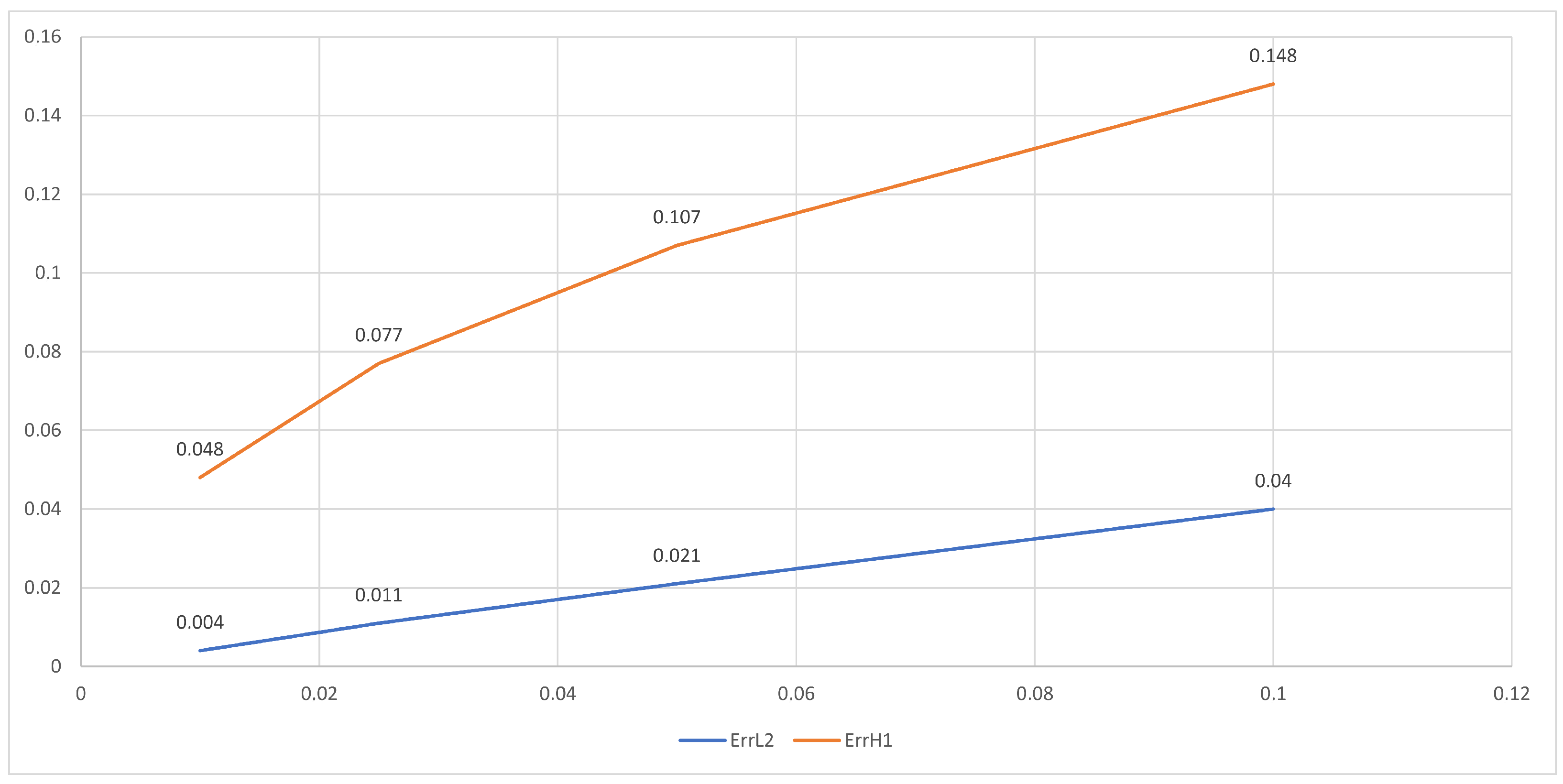
ErrH1	0.148	0.107	0.077	0.048

(see also Figure 2), we investigate the dependence of the relative error on the parameter $\delta$ characterizing inclusion’s width (for $d=0.5$, $p=0$). They show good approximation of the initial problem (with non-zero width) by the thin inclusion problem in both $L_2$- and $H^1$-norms.

Table 2. Relative error vs. p for the case $d=0.5$, $\delta =0.01$.

	$\mathit{p}=-2$	$\mathit{p}=-1$	$\mathit{p}=0$	$\mathit{p}=1$	$\mathit{p}=2$
ErrL2	0.001	0.004	0.005	0.008	0.019
ErrH1	0.013	0.043	0.048	0.056	0.086

shows the dependence of relative error on the parameter p, which characterizes the roughness of the inclusion. It can be seen that the approximation for the soft inclusions is better than the approximation for the hard inclusions. This feature can be explained by the fact that in the case of the hard inclusion, there are large stresses in the vertices of the inclusions and in the places of great curvature. It should be noted that, in [43], the asymptotic behavior of the solution near the tip of the rigid line inclusion was studied in the case of two-dimensional homogeneous isotropic linearized elasticity. In [44], the numerical method of solving bulk and thin rigid inclusion problems was proposed.

Table 3. Relative error vs. d for the case $\delta =0.01$, $p=0$.

	0	0.1	0.2	0.3	0.4	0.5
ErrL2	0.002	0.004	0.005	0.005	0.004	0.005
ErrH1	0.054	0.051	0.052	0.05	0.048	0.048

illustrates the dependence of the relative errors on the parameter d that characterizes the curvature of the inclusion (the case of $d=0$ corresponds to the rectilinear inclusion, and the case $d=0.5$ corresponds to the sinusoid with an amplitude equal to one).

Let us investigate a mesh sensitivity analysis. Let $h.min$ and $h.max$ denote the minimal and maximal sizes of mesh triangles of the domain $\mathsf{\Omega }$.

Table 4. Relative error vs. mesh sizes $h.min$ and $h.max$ for the case $\delta =0.01$, $p=0$.

$\mathit{h}.\mathit{min}$	$\mathit{h}.\mathit{max}$	ErrL2	ErrH1
0.08	0.28	0.013	0.074
0.03	0.14	0.005	0.057
0.013	0.076	0.005	0.051
0.009	0.048	0.005	0.049
0.005	0.042	0.004	0.048

presents numerical calculations in dependence of mesh sizes. Again, it shows a good approximation of the initial problem (with non-zero width) by the thin inclusion problem in both $L_2$- and $H^1$-norms.

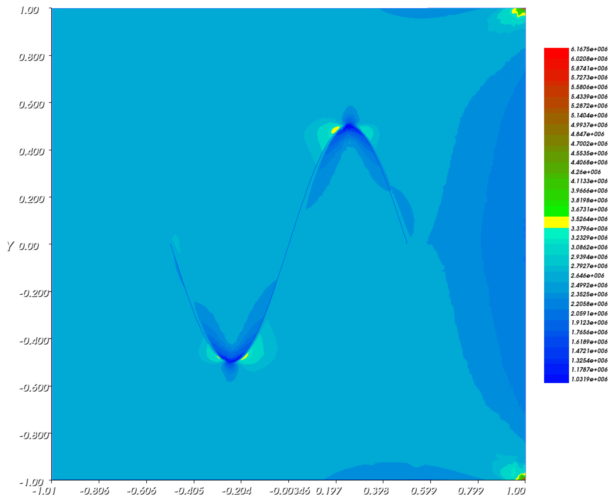
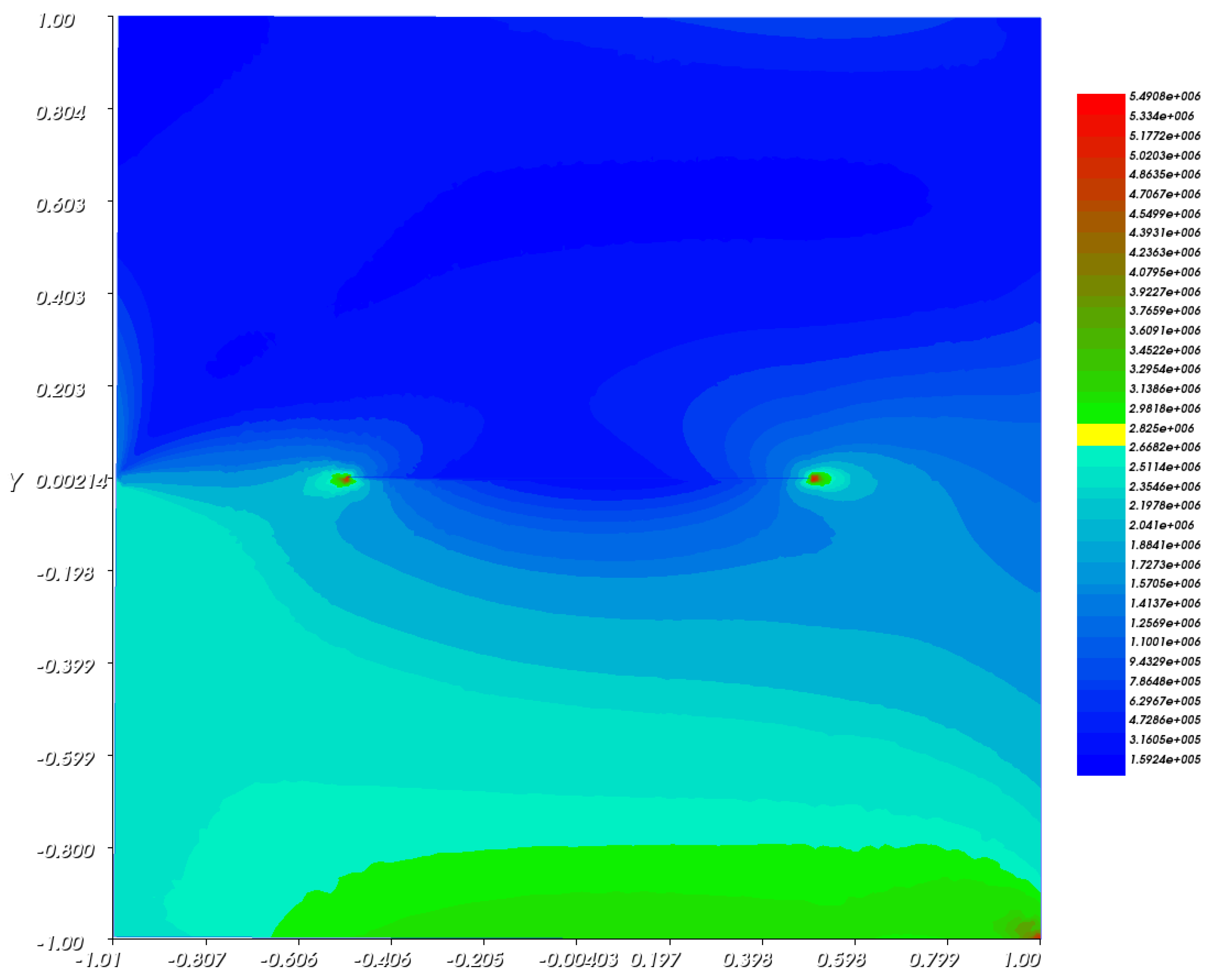
At last, the resulting deformations in the Lagrange coordinates (with the tenfold amplification factor) and the distribution of the von Mises stresses are depicted in Figure 3 for the curvilinear inclusion (case $d=0.5$) for the applied loading as stated at the beginning of Section 6 and in Figure 4 for the rectilinear inclusion (case $d=0$) for the non-symmetric tensile loading $g=(g_1,0)$, where $g_1=-{10}^{-3}{\mu }_m$ on ${\mathsf{\Gamma }}_N^3\cap \{y_2<0\}$ and $g_1=0$ on $({\mathsf{\Gamma }}_N^3\cap \{y_2>0\})\cup {\mathsf{\Gamma }}_N^2\cup {\mathsf{\Gamma }}_N^1$. It can be seen that, in the case of the curvilinear inclusion, there is a singularity in the vicinity of the curved part of the inclusion, while in the case of the rectilinear inclusion singularity, it appears only in the vicinity of its tips. This means that the curvature k plays an essential role in modeling curvilinear inclusions.

7. Conclusions

By using a variational approach, the model of the elastic body containing strictly inside the curvilinear rod-like thin inclusion has been derived. The model approximates the equilibrium problem of the non-homogeneous elastic body with the narrow inclusion, the width and elastic properties of which depend on the small parameter $\delta$ (the width is proportional to $\delta$, while elastic properties are proportional to ${\delta }^{-1}$). The approximated model has a variational formulation. This allows the application of the standard finite-element method in order to compare solutions of the initial problem and approximated one. Numerical experiments show a good approximation in both $L_2$-norm and $H^1$-norm as the parameter $\delta$ goes to zero.

In the future, it is planned to perform an asymptotic procedure for other types of dependence of the elastic properties of the inclusion on the small parameter characterizing its width and justify models of thin inclusion of different types (beam-like, rigid, etc.).

References

1. Fankina, I.V.; Furtsev, A.I.; Rudoy, E.M.; Sazhenkov, S.A. Asymptotic modeling of curvilinear narrow inclusions with rough boundaries in elastic bodies: Case of a soft inclusion. Sib. Electron. Math. Rep. 2022, 19, 935–948. [Google Scholar]
2. Furtsev, A.; Rudoy, E. Variational approach to modeling soft and stiff interfaces in the Kirchhoff-Love theory of plates. Int. J. Solids Struct. 2020, 202, 562–574. [Google Scholar] [CrossRef]
3. Rudoy, E.M. Asymptotic justification of models of plates containing inside hard thin inclusions. Technologies 2017, 8, 59. [Google Scholar] [CrossRef]
4. Itou, H.; Khludnev, A.M. On delaminated thin Timoshenko inclusions inside elastic bodies. ZAMM Z. Angew. Math. Mech. 2016, 24, 4980–4993. [Google Scholar] [CrossRef]
5. Khludnev, A.; Negri, M. Crack on the boundary of a thin elastic inclusion inside an elastic body. ZAMM Z. Angew. Math. Mech. 2012, 95, 341–354. [Google Scholar] [CrossRef]
6. Khludnev, A. On thin inclusions in elastic bodies with defects. Z. Angew. Math. Phys. 2019, 70, 45. [Google Scholar] [CrossRef]
7. Khludnev, A. T-shape inclusion in elastic body with a damage parameter. J. Comput. Appl. Math. 2021, 393, 113540. [Google Scholar] [CrossRef]
8. Khludnev, A. Non-coercive problems for Kirchhoff–Love plates with thin rigid inclusion. Z. Angew. Math. Phys. 2022, 73, 54. [Google Scholar] [CrossRef]
9. Lazarev, N.P. Equilibrium problem for a thermoelastic Kirchhoff-Love plate with a delaminated flat rigid inclusion. Philos. Trans. R. Soc. A 2022, 380, 20210363. [Google Scholar] [CrossRef] [PubMed]
10. Lazarev, N.P.; Kovtunenko, V.A. Signorini-type problems over non-convex sets for composite bodies contacting by sharp edges of rigid inclusions. Mathematics 2022, 10, 250. [Google Scholar] [CrossRef]
11. Khludnev, A. Junction problem for thin elastic and volume rigid inclusions in elastic bod. Philos. Trans. R. Soc. A 2022, 380, 20210360. [Google Scholar] [CrossRef]
12. Khludnev, A. On the Crossing Bridge between Two Kirchhoff–Love Plates. Axioms 2023, 12, 120. [Google Scholar] [CrossRef]
13. Khludnev, A. Asymptotic analysis of thin elastic junction between two elastic bodies. Appl. Anal. 2023, 102, 800–814. [Google Scholar] [CrossRef]
14. Baranova, S.; Mogilevskaya, S.G.; Nguyen, T.H.; Schilling, D. Higher-order imperfect interface modeling via complex variables based asymptotic analysis. Int. J. Eng. Sci. 2021, 57, 103399. [Google Scholar]
15. Fankina, I.V.; Furtsev, A.I.; Rudoy, E.M.; Sazhenkov, S.A. Multiscale analysis of stationary thermoelastic vibrations of a composite material. Philos. Trans. R. Soc. A 2022, 380, 20210354. [Google Scholar]
16. Mokhtari, H.; Rahmani, L. Asymptotic modeling of the behavior of a reinforced plate governed by a full von Karman thermo-elastic system with nonlinear thermal coupling. Ann. Univ. Ferrara Sez. VII Sci. Mat. 2021, 67, 387–414. [Google Scholar] [CrossRef]
17. Serpilli, M.; Dumont, S.; Rizzoni, R.; Lebon, F. Interface Models in Coupled Thermoelasticity. Technologies 2021, 9, 17. [Google Scholar] [CrossRef]
18. Benveniste, Y.; Miloh, T. Imperfect soft and stiff interfaces in two-dimensional elasticity. Mech. Mater. 2001, 33, 309–323. [Google Scholar] [CrossRef]
19. Bessoud, A.-L.; Krasucki, F.; Serpilli, M. Plate-like and shell-like inclusions with high rigidity. Comptes Rendus Math. 2009, 346, 697–702. [Google Scholar]
20. Ljulj, M.; Tambaca, J. 3D structure—2D plate interaction model. Math. Mech. Solids 2019, 24, 3354–3377. [Google Scholar] [CrossRef]
21. Serpilli, M.; Rizzoni, R.; Rodríguez-Ramos, R.; Lebon, F.; Dumont, S. A novel form of imperfect contact laws in flexoelectricity. Compos. Struct. 2022, 300, 116059. [Google Scholar] [CrossRef]
22. Bessoud, A.-L.; Krasucki, F.; Michaille, G. Multi-materials with strong interface: Variational modelings. Asymptot. Anal. 2012, 61, 1–19. [Google Scholar] [CrossRef] [Green Version]
23. Dumont, S.; Lebon, F.; Raffa, M.L.; Rizzoni, R. Towards nonlinear imperfect interface models including micro-cracks and smooth roughness. Ann. Solid Struct. Mech. 2017, 9, 13–27. [Google Scholar] [CrossRef] [Green Version]
24. Fouchal, F.; Lebon, F.; Raffa, M.L.; Vairo, G. An interface model including cracks and roughness applied to masonry. Open Civ. Eng. J. 2014, 8, 263–271. [Google Scholar] [CrossRef]
25. Kunets, Y.I.; Matus, V.V. Asymptotic approach in the dynamic problems of the theory of elasticity for bodies with thin elastic inclusions. J. Math. Sci. 2023, 270, 87–106. [Google Scholar] [CrossRef]
26. Mokhtari, H.; Rahmani, L. Asymptotic modeling of a reinforced plate with a thin layer of variable thickness. Meccanica 2022, 57, 2155–2172. [Google Scholar] [CrossRef]
27. Dong, H.; Zheng, X.; Cui, J.; Nie, Y.; Yang, Z.; Ma, Q. Multi-scale computational method for dynamic thermo-mechanical performance of heterogeneous shell structures with orthogonal periodic configurations. Comput. Methods Appl. Mech. Eng. 2019, 354, 143–180. [Google Scholar] [CrossRef]
28. Ma, Q.; Li, Z.; Cui, J. Multi-scale asymptotic analysis and computation of the elliptic eigenvalue problems in curvilinear coordinates. Comput. Methods Appl. Mech. Eng. 2018, 340, 340–365. [Google Scholar] [CrossRef]
29. Ma, Q.; Cui, J.; Li, Z.; Wang, Z. Second-order asymptotic algorithm for heat conduction problems of periodic composite materials in curvilinear coordinates. J. Comput. Appl. Math. 2016, 306, 87–115. [Google Scholar] [CrossRef]
30. Khludnev, A.M.; Kovtunenko, V.A. Analysis of Cracks in Solids; WIT-Press: Southampton, UK, 2000. [Google Scholar]
31. Nečas, J. Direct Methods in the Theory of Elliptic Equations; Springer: Berlin/Heidelberg, Germany, 2012. [Google Scholar]
32. Rudoy, E.M.; Itou, H.; Lazarev, N.P. Asymptotic Justification of the Models of Thin Inclusions in an Elastic Body in the Antiplane Shear Problem. J. Appl. Ind. Math. 2021, 15, 129–140. [Google Scholar] [CrossRef]
33. Rudoy, E. First-order and second-order sensitivity analyses for a body with a thin rigid inclusion. Math. Methods Appl. Sci. 2016, 39, 4994–5006. [Google Scholar] [CrossRef]
34. Rudoy, E.; Shcherbakov, V. First-Order Shape Derivative of the Energy for Elastic Plates with Rigid Inclusions and Interfacial Cracks. Appl. Math. Optim. 2021, 84, 2775–2802. [Google Scholar] [CrossRef]
35. Freddi, L.; Morassi, A.; Paroni, R. Thin-Walled Beams: The Case of the Rectangular Cross-Section. J. Elast. 2004, 76, 45–66. [Google Scholar] [CrossRef]
36. Gaudiello, A.; Sili, A. Limit models for thin heterogeneous structures with high contrast. J. Differ. Equ. 2021, 302, 37–63. [Google Scholar] [CrossRef]
37. Nazarov, S.A. Weighted anisotropic Korn’s inequality for a junction of a plate and a rod. Sb. Math. 2004, 195, 553–583. [Google Scholar] [CrossRef]
38. Baranova, S.; Mogilevskaya, S.G. On the Bovik–Benveniste methodology and related approaches for modelling thin layers. Philos. Trans. R. Soc. A 2022, 380, 20210420. [Google Scholar] [CrossRef] [PubMed]
39. Fankina, I.V.; Furtsev, A.I.; Rudoy, E.M.; Sazhenkov, S.A. The homogenized quasi-static model of a thermoelastic composite stitched with reinforcing threads. J. Comput. Appl. Math. 2023, 434, 115346. [Google Scholar] [CrossRef]
40. Kushch, V.I.; Mogilevskaya, S.G. Higher order imperfect interface models of conductive spherical interphase. Math. Mech. Solids 2022. [Google Scholar] [CrossRef]
41. Ventcel, A.D. On boundary conditions for multi-dimensional diffusion processes. Theory Probab. Appl. 1959, 42, 164–177. [Google Scholar]
42. Hecht, F. New development in FreeFem++. J. Numer. Math. 2012, 20, 251–265. [Google Scholar] [CrossRef] [Green Version]
43. Itou, H.; Khludnev, A.M.; Rudoy, E.M.; Tani, A. Asymptotic behaviour at a tip of a rigid line inclusion in linearized elasticity. ZAMM Z. Angew. Math. Mech. 2012, 92, 716–730. [Google Scholar] [CrossRef]
44. Rudoy, E.M. On numerical solving a rigid inclusions problem in 2D elasticity. ZAMP Z. Angew. Math. Phys. 2017, 68, 19. [Google Scholar] [CrossRef]
Figure 1. Domain configuration.
Mathematics 11 03447 g001
Figure 2. Relative error vs. δ for the case d = 0.5 , p = 0 .
Mathematics 11 03447 g002
Figure 3. Deformed body with the sinusoidal inclusion and distribution of the von Mises stresses.
Mathematics 11 03447 g003
Figure 4. Deformed body with the rectilinear inclusion and distribution of the von Mises stresses.
Mathematics 11 03447 g004