Abstract
Fuzzy rough set theory has been successfully applied to many attribute reduction methods, in which the lower approximation set plays a pivotal role. However, the definition of lower approximation used has ignored the information conveyed by the upper approximation and the boundary region. This oversight has resulted in an unreasonable relation representation of the target set. Despite the fact that scholars have proposed numerous enhancements to rough set models, such as the variable precision model, none have successfully resolved the issues inherent in the classical models. To address this limitation, this paper proposes an unsupervised attribute reduction algorithm for mixed data based on an improved optimal approximation set. Firstly, the theory of an improved optimal approximation set and its associated algorithm are proposed. Subsequently, we extend the classical theory of optimal approximation sets to fuzzy rough set theory, leading to the development of a fuzzy improved approximation set method. Finally, building on the proposed theory, we introduce a novel, fuzzy optimal approximation-set-based unsupervised attribute reduction algorithm (FOUAR). Comparative experiments conducted with all the proposed algorithms indicate the efficacy of FOUAR in selecting fewer attributes while maintaining and improving the performance of the machine learning algorithm. Furthermore, they highlight the advantage of the improved optimal approximation set algorithm, which offers higher similarity to the target set and provides a more concise expression.
Keywords:
fuzzy rough set; granular computing; optimal approximation set; unsupervised attribute reduction MSC:
68T37; 03E72; 62H30
1. Introduction
Since the introduction of rough sets by Pawlak [1] in 1982, attribute reduction, also known as feature selection, has emerged as an important research direction in rough set applications [2,3,4]. Attribute reduction algorithms rooted in classical rough set theory are often termed positive region reduction algorithms [5,6,7], which use knowledge granules (equivalence classes) in the data attributes to approximate the target set. Among these, the equivalence classes that are wholly contained within the target set are designated as lower approximations, while those that have intersections with the target set are denoted as upper approximations. The difference between the lower and upper approximations is referred to as the boundary region. However, the classical rough set model cannot be directly applied to numerical data types. Concurrently, fuzzy set theory has achieved success in numerous domains, such as fuzzy logic systems [8,9] and pattern recognition. To address the limitation of rough sets in handling numerical data, Dubois and Prade [10,11] integrated rough set models with fuzzy set theory and proposed fuzzy rough sets. Reduction algorithms based on fuzzy rough sets employ similarity kernel functions to ensure more efficacious attribute reduction without sacrificing the information contained in the data. Consequently, a plethora of scholars have conducted in-depth and extensive research on reduction algorithms predicated on fuzzy rough sets [12,13,14,15,16,17,18,19,20,21,22,23,24,25,26,27]. For instance, Hu et al. [16] devised a heuristic algorithm that guarantees the algorithm’s convergence by proposing a novel fuzzy rough set. Yuan et al. [20] extended the supervised fuzzy rough set algorithm to unsupervised fuzzy rough set attribute reduction.
However, lower approximation theory, which is widely employed within these models, still possesses significant limitations. Traditionally, lower approximation theory stipulates that knowledge granules must be entirely contained within the target set; failing this, it is inferred that the target set cannot be represented by the extant knowledge granules. This criterion overlooks the information in the boundary region, resulting in an inability to accurately describe the dependencies among many attributes. In order to address these issues, scholars have proposed a plethora of refined models. Ziarko et al. [28] introduced the variable precision rough set model. Its fundamental concept entails establishing a tolerance threshold within the traditional rough set model, which allows knowledge granules that fall under this threshold to be regarded as lower approximations of the target set. Chen et al. [29] incorporated a rough membership function and approximation parameters from variable precision rough sets into the multigranulation environment, establishing a model known as the variable precision multigranulation rough set. Dai and Li [30,31] investigated the VPRS model in the context of a double universe, focusing on its structures and properties. These models share a common characteristic, which is the relaxation of the inclusion criteria for lower approximations to a certain extent by setting parameters. However, when knowledge granules still cannot satisfy the relatively relaxed inclusion criteria, these models crudely consider the knowledge granules to have no association with the target set. In reality, the refined models have not fundamentally addressed the issues faced by rough sets, but have only provided a degree of alleviation to the problem.
Several scholars have proposed the utilization of optimal approximation sets as substitutes for lower approximation sets during the reduction process [32,33,34,35,36,37]. The primary objective is to identify the set that most accurately represents the target set. An optimal approximation set comprises the lower approximation of the target set and a segment of the boundary area, enabling effective utilization of the information derived from this region. By leveraging the similarity between knowledge granules and the target set to replace the lower approximation present in traditional rough sets, their relationship can be precisely described using a similarity function, irrespective of whether the knowledge granules are encompassed within the target set. This approach effectively resolves the issues encountered in rough sets. Furthermore, optimal approximation sets can also mitigate these same challenges faced by variable-precision models and other similar models when applied to practical problems. Despite their potential, however, current models of optimal approximation sets present several limitations. For example, they are rooted in traditional rough set theory and are consequently only applicable to categorical data. Furthermore, the current methods used to find optimal approximation sets fall short of identifying the most similar representation of the target set in a theoretical sense. These shortcomings not only restrict the broad applicability of optimal approximation sets but also prevent them from accurately embodying the target.
To tackle the challenges discussed above, this study presents modifications and extensions to the concept of optimal approximation sets. Concomitant with this endeavor, we also propose a new unsupervised attribute reduction approach that leverages these improved fuzzy optimal approximation sets. Primarily, we have upgraded traditional optimal approximation sets theory, proposing a more advanced version of this theory along with the associated theorems. In a further amplification, the traditional ambit of optimal approximation sets theory has been broadened to incorporate elements of fuzzy set theory, resulting in a new theory for fuzzy optimal approximation sets. Building on the foundation of the refined optimal approximation set model, we proposed two new algorithms: an improved optimal approximation set algorithm (IOAS) and a fuzzy improved optimal approximation set algorithm (FIOAS). Lastly, leveraging the fuzzy optimal approximation set model, we proposed a novel attribute importance function and developed a unique algorithm for unsupervised attribute reduction, namely FOUAR. To test the validity of IOAS and FOUAR, we carried out experiments on 30 different datasets. The results showed that IOAS can identify closer matches to the target set and can also minimize the size of optimal approximation sets. On the other hand, FOUAR showed its ability to pick fewer, yet higher-quality attributes. The algorithm FOUAR also demonstrated its capacity to maintain and even enhance the accuracy of subsequent machine learning tasks. Moreover, the outcomes of parameter experiments showed that FOUAR is quite robust against changes in parameters. Hypothesis tests performed suggest that there are notable differences between FOUAR and most other algorithms, with FOUAR consistently achieving the top ranks.
The main contributions of this paper are as follows:
- (1)
- We extend the existing theory of optimal approximation sets to create a theory of fuzzy optimal approximation sets. This enables their application to mixed data types.
- (2)
- We introduce improved algorithms for solving optimal approximation sets, known as IOAS and FIOAS. These enhanced methods enable higher similarity to the target set and produce smaller optimal approximation sets.
- (3)
- We propose an unsupervised attribute reduction algorithm based on fuzzy optimal approximation sets. This algorithm is capable of selecting fewer attributes while maintaining the accuracy of classification and clustering tasks.
The remainder of this paper is organized as follows: Section 2 introduces the preliminary information on rough set theory. Progressing to Section 3, we discuss optimal approximation set theory and its improved algorithm. Thereafter, in Section 4, we extend the classical theory of optimal approximation sets and related definitions to fuzzy set theory, and propose an algorithm for fuzzy optimal approximation sets. Transitioning to Section 5, we present a series of theories and definitions related to fuzzy optimal approximation sets, as well as an unsupervised attribute reduction algorithm for mixed data based on fuzzy optimal approximation sets. Additionally, an example is provided to illustrate the proposed method. Section 6 presents the experimental results. Finally, conclusions are drawn in Section 7.
2. Relevant Concepts
Definition 1
([1]). Let U be a finite universe, and R be an equivalence relation on U. Then, the pair is called an approximation space. The equivalence classes determined by the equivalence relation R are referred to as the basic knowledge on the approximation space , which can be denoted as , where .
Definition 2
([1]). Let be an approximation space, where R is an equivalence relation on U. For any subset , the lower approximation of X is defined as , and the upper approximation of X is defined as .
Definition 3
([38]). Let , for any , if satisfies
- Boundedness, , , and only if ;
- Symmetry, ;
- , , ,
then, is called the similarity degree between sets X and Y. In this paper, let .
3. Improvement Based on Optimal Approximation Set
In this section, we mainly introduce the calculation method of the optimal approximation set, the improved algorithm of the optimal approximation set, and its related theorems.
3.1. Optimal Approximation Set
For a target set , its lower and upper approximations are denoted by and , respectively. The optimal approximation set is defined as the set with the highest similarity to X between the lower and upper approximations and can be represented using the basic knowledge in the approximation space. Compared to other approximation sets, the optimal approximation set ensures a high degree of approximation accuracy for the target set without necessitating manual parameter adjustments. The definition of the optimal approximation set is provided below.
Definition 4.
Let be a target, where is the power set of . For any , if there exists such that where , and , then, is called the optimal approximation set of X.
For convenience, in this paper, we denote as .
Given an approximation space , , let , , and . Then, for any , X can be approximated and characterized by . Based on the above description, a theorem for computing the optimal approximation set of the target set X is provided in [36].
Theorem 1
([36]). Let be an approximation space, . If , then, is called the optimal approximation set of X.
Theorem 1 identifies a relatively high-precision approximation of the target set X. Here is an explanation for Theorem 1: If we consider as the approximation of X, then the similarity can be calculated as follows: . After derivation, we get: . In this context, if we desire an increase in the similarity relative to , then we need to identify an instance where . Given this, we can deduce:
represent it with similarity and we get:
Following this idea, we can filter the knowledge from that meets the condition and assemble it into . In this case, the similarity between and X is greater than the similarity between and X. Consequently, we have found a set that can better represent X as an approximation set compared to .
Theorem 1 identifies a high-precision approximation set that offers a more reasonable representation of the target set. A corresponding example illustrating this theorem is provided below.
Example 1.
From Table 1, we can infer that the decision attribute d has the following equivalence classes: and . Next, we will consider as the target set, and Theorem 1 will be employed to compute the optimal approximation set. Then, we will utilize the obtained results to illustrate the limitations of Theorem 1.
Utilizing the equivalence relation R, we derive the partition of U under R as follows: , where , , and . By applying Theorem 1, we compute the optimal approximation set :
Given that , and in accordance with the definition of , we obtain: , and . As both values exceed α, we deduce that . Subsequently, the similarity can be computed as:
Thus, the optimal approximation set of is given by .
However, there exists an alternative such that
According to the definition of upper approximation, the upper approximation of is , which is equal to .
In fact, the subset allows to achieve a higher degree of approximation accuracy to the target set X compared to . Theorem 1 only identifies a set that can better characterize the target set X than , and does not truly verify whether is the optimal approximation set that maximizes the similarity. In the next subsection, we will present the relevant theorem for optimal approximation sets and an improved algorithm.

Table 1.
Decision information system.
Table 1.
Decision information system.
| U | d | |||
|---|---|---|---|---|
| 1 | 0 | 1 | 0 | |
| 1 | 0 | 1 | 0 | |
| 1 | 0 | 1 | 0 | |
| 1 | 0 | 1 | 0 | |
| 1 | 0 | 1 | 0 | |
| 1 | 0 | 1 | 1 | |
| 1 | 0 | 1 | 1 | |
| 0 | 1 | 0 | 1 | |
| 0 | 1 | 0 | 1 | |
| 0 | 1 | 0 | 1 | |
| 0 | 1 | 0 | 1 | |
| 0 | 1 | 0 | 0 | |
| 0 | 1 | 0 | 0 | |
| 0 | 1 | 0 | 0 | |
| 0 | 1 | 0 | 0 | |
| 0 | 1 | 0 | 0 | |
| 0 | 0 | 1 | 1 | |
| 0 | 0 | 1 | 1 |
3.2. Improvement of Optimal Approximation Set
In this subsection, we mainly introduce the calculation method of the optimal approximation set, the improved algorithm of the optimal approximation set, and its related theorems.
Lemma 1
([17]). For any positive constants , if , then we have .
Now, we denote:
- For the target set X, let ;
- Let denote , and denote ;
- Let denote .
The following is the theorem regarding the existence of the optimal approximation set.
Theorem 2.
Let , if , then, we have .
Proof of Theorem 2.
Since and . Applying Lemma 1, we have
thus, we can obtain . □
From Theorem 2, for , if there exists such that
then, according to Lemma 1, the following result can be obtained:
According to the conclusion deduced based on Theorem 1 in A, the following result can be derived:
Thus, the inequality (Equation (2)) can be expressed by the similarity (Equation (3)), which yields .
The above conclusion indicates that removing some of the less informative elements from can actually improve the approximation accuracy. Therefore, when we sort all , in ascending order as , Lemma 1 and Theorem 2 can be employed to derive the following theorem for identifying the optimal approximation set.
Theorem 3.
For a given , where , if there exists , then the following is true:
Proof of Theorem 3.
Mathematical induction can be used to prove that
When , according to the assumption of the theorem, we know that , so we have , and .
Based on Lemma 1, we have , and . When , if and , then , which implies that . From Lemma 1, we have and . Using mathematical induction, we can obtain . □
In light of Theorem 3, we now propose an improved algorithm for determining the optimal approximation set, as given in Algorithm 1, namely, the improved algorithm for optimal approximation set (IOAS).
| Algorithm 1: IOAS |
 |
Example 2
(Continued from Example 1). We will apply the improved algorithm for the optimal approximation set (IOAS) to re-evaluate the following example.
By following the step 2 in Algorithm 1, we have:
According to step 4 in Algorithm 1, and , we can obtain . Then, following Step 5 in IOAS, update to and to . Based on steps 7–9 and step 3, since
is removed from and . Finally, we obtain the optimal approximation set , and the resulting similarity is
The improved algorithm provides a higher similarity value compared to the result obtained through Theorem 1. Additionally, the algorithm has effectively reduced the size of the optimal approximation set. As a result, it provides a more accurate and concise representation of the target set .
4. Improved Algorithm Based on Fuzzy Optimal Approximation Set
In this section, we have extended the classical theory of optimal approximation sets to fuzzy set theory, and proposed an algorithm for solving the optimal approximation sets of fuzzy sets based on this extension.
4.1. Relative Definition
In this paper, we represent a fuzzy information system as , which is a fuzzy decision information system where U is a non-empty finite domain, A is a non-empty finite set of attributes that satisfies and , V is the value range of all attribute values, and f is a mapping that fulfills . Additionally, a fuzzy information system without a decision is denoted as .
In situations without ambiguity, for the sake of simplicity, we represent as , where R denotes the equivalence or similarity relation, and C refers to either an attribute set or an attribute subset.
Definition 5
([10,39]). A fuzzy relation R on U is defined as . , the membership degree indicates the degree to which x and y have a relationship R. The set of all fuzzy relations on U is denoted as .
Suppose , , if it satisfies the following conditions
- Reflexivity ;
- Symmetry ;
- Transitivity ,
then R is called a fuzzy equivalence relation on U. Furthermore, if R only satisfies reflexivity and symmetry, then R is called a fuzzy similarity relation on U. , we have
- ;
- ;
- .
Definition 6
([10,39]). Let be a fuzzy information system, and R be a fuzzy similarity relation on U. For any , the lower approximation and upper approximation of X are a pair of fuzzy sets on U whose membership functions, respectively, are
Definition 7.
Let be a fuzzy information system, for any fuzzy sets , the fuzzy similarity degree S between X and Y is defined as follows:
where the represents the cardinality of a set.
Definition 8.
Let be a fuzzy information system. For any , is the fuzzy similarity relation on U, is the fuzzy similarity class under B, and is the power set of all similarity classes under B. Given a fuzzy target set , for any , if there exists , denoted as , such that . Then, is called the fuzzy optimal approximation set about X, where .
Similarly to the previous section, for a set of fuzzy sets T, we denote as .
Theorem 4.
Let be a fuzzy information system, where R is the fuzzy equivalence relation on U. For , if , then, is the fuzzy optimal approximation set of X.
Proof of Theorem 4.
Similar to Theorem 1. □
4.2. Improved Fuzzy Optimal Approximation Set Model
In this subsection, we propose an enhanced algorithm for optimal approximation sets and illustrate the algorithm using an example.
To ensure accurate data processing regardless of the difference of data, we adopt the maximum-minimum normalization method [40] for numerical data in the dataset, which transforms the data into the interval . The calculation formula is as follows:
where and are the maximum and minimum values of attribute . This paper employs a kernel function that is capable of handling mixed data types simultaneously. The specific function is presented below:
where represents the fuzzy similarity relationship between attributes, and is a conditionally fuzzy similarity radius, with the specific calculation formula as follows:
where is the standard deviation of attribute , and the preset parameter is used to adjust the fuzzy similarity radius.
In order to compute the optimal approximation set of a fuzzy set, similar to IOAS, this paper proposes a fuzzy improved optimal approximation set algorithm (FIOAS) as Algorithm 2.
| Algorithm 2: FIOAS |
 |
Next, we provide an example to illustrate the effectiveness of FIOAS in computing the optimal approximation set of the target set X.
Example 3.
Let be a fuzzy information system, as shown in Table 2. Among the attributes, is nominal and and are numerical. Given a fuzzy target set , we calculate the optimal approximation set of X using FIOAS as follows: First, we normalize the data using min-max normalization (Equation (7)). Next, we calculate the fuzzy similarity radius using (Equation (9)) with , resulting in and . Finally, we set .
Thus, the fuzzy similarity matrices for any are obtained using (Equation (8)) as follows:
.
Therefore, the fuzzy similarity matrix of can be derived as follows:
From the matrix , we can deduce the following results:
Using (Equation (4)) from definition 6, we can derive the lower approximation of X, which can be represented as a fuzzy set:
Since , we can determine that by utilizing Theorem 4. Then, according to Step 4 in FIOAS, we obtain . Based on steps 5–8, we can ascertain and , which implies that FIOAS excludes and form in this iteration. Furthermore, in the next iteration, we can obtain and . Finally, the optimal approximation set of X can be derived as follows:
and the similarity can be calculated as .
However, for , the similarity for target set X is . This demonstrates the effectiveness of FIOAS in computing the optimal approximation set of X on fuzzy sets.
Table 2.
Mixed Data Table.
Table 2.
Mixed Data Table.
| U | |||
|---|---|---|---|
| 1 | 0.2 | 12.1 | |
| 1 | 0.3 | 11.1 | |
| 2 | 0.7 | 3.2 | |
| 2 | 0.7 | 3.3 | |
| 3 | 0.8 | 2.6 |
5. Unsupervised Algorithm Based on Fuzzy Optimal Approximation Set
In this section, we propose a fuzzy optimal approximation-based unsupervised attribute reduction algorithm for mixed data (abbreviated as FOUAR). Subsequently, we analyze the algorithmic complexity of FOUAR. Finally, an example is presented to illustrate the computation process of FOUAR, with a comparative analysis of the reduction results alongside those of FRUAR.
5.1. Relative Definitions and Model
In the following, we utilize the optimal approximation set model to define the attribute importance function and attribute relevance function.
Definition 9.
Let be a fuzzy information system, where R is the fuzzy equivalence relation on U. For any . are all fuzzy sets under Q, and are all fuzzy sets under P. Then, the optimal approximation set of relative to P can be denoted as , and the fuzzy optimal approximation dependency of P to can be defined as
Then, the fuzzy optimal approximation dependency of P relative to Q can be defined as
Definition 10.
Let be a fuzzy information system, where R is the fuzzy equivalence relation on U. For any , the relevance of B on all single attribute subsets is defined as
Ultimately, we define reduction based on the importance function and relevance function.
Definition 11.
Let be a fuzzy information system, where R is the fuzzy equivalence relation on U. For any , we say that B is a reduction of C, if B satisfies
- ,
According to the aforementioned theorems and definitions, an unsupervised attribute reduction algorithm for mixed data based on fuzzy optimal approximation sets is proposed in this paper as Algorithm 3.
5.2. Complexity Analysis
In this section, we will analyze the complexity of the FOUAR algorithm.
The time complexity of the FOUAR algorithm can be analyzed as follows. In the first for-loop, steps 2–4 of the algorithm, we calculate the similarity matrix for each attribute , which takes time. In steps 5–26, The while loop iterates h times, where h is the size of the current candidate attribute set B. Then, in steps 7–17 of the algorithm, for each attribute , we calculate and for all , which takes time. Finally, In steps 18 and 19 of the algorithm, we calculate the relevance degree , which takes time. Therefore, the time complexity of the FOUAR algorithm can be expressed as .
Compared to traditional unsupervised attribute reduction algorithms, our method tends to be more time-consuming overall. This is because our algorithm spends more time computing the optimal approximate sets for each fuzzy partition of an attribute, which is more resource-intensive than computing the lower approximations used in traditional methods.
| Algorithm 3: FOUAR |
 |
5.3. Specific Example
Example 4.
According to Algorithm 3, we apply FOUAR to reduce the data in Table 3. In this table, attributes and represent the same values under different temperature scales (Fahrenheit and Celsius). Thus, and are considered redundant attributes.
Let R denote the set of attribute reductions with an initial condition , and let .
First, we use the max-min normalization method to standardize the numerical data in Table 3 and calculate the fuzzy similarity matrix corresponding to each attribute, denoted as , , , , . Then, for calculating the optimal approximation set of all fuzzy sets , we should first calculate:
- ,
- and are also calculated to be 1. Following the same procedure, we can see that
- ,
- ,
- ⋯
- ,
- .
- Similarly, we can obtain , , for .
Using Algorithm 2, we can obtain the optimal approximation set for each fuzzy set under each attribute , and then use the obtained optimal approximation sets to calculate the degree of dependency of each attribute.
By calculating the optimal approximation dependence, we have:
- ,
- , ,
- , .
- Thus, the relevance degree can be calculated as
- .
- Similarly, we can obtain:
- , ,
- , .
- Therefore, can be obtained as follows:
- .
- Hence, can be selected as the attribute corresponding to the maximum attribute relevance and added to R. At this point, .
Similarly, after recalculating , , we use FIOAS to obtain the optimal approximation set for each attribute under R. Then, we recalculate the dependency degree, which can yield:
- ,
- , ,
- , .
- Then, calculate the relevance .
- We can similarly obtain that ,
- , and .
- Since , we select the attribute corresponding to the maximum and obtain .
Similarly, further iteration leads to . When the final iteration is performed, we have , .
Table 3.
Mixed Data Table.
Table 3.
Mixed Data Table.
| U | |||||
|---|---|---|---|---|---|
| A | 2 | 38.0 | 100.4 | 2 | |
| A | 1 | 36.2 | 97.2 | 1 | |
| A | 1 | 36.1 | 97.0 | 1 | |
| A | 1 | 36.3 | 97.3 | 1 | |
| A | 1 | 36.4 | 97.5 | 1 | |
| B | 2 | 39.2 | 102.6 | 1 | |
| B | 2 | 39.3 | 102.6 | 1 | |
| B | 2 | 38.4 | 101.1 | 1 | |
| B | 2 | 39.2 | 102.6 | 1 | |
| B | 2 | 38.1 | 100.6 | 1 | |
| B | 2 | 36.1 | 96.9 | 1 | |
| B | 2 | 36.4 | 97.5 | 1 | |
| B | 2 | 36.3 | 97.3 | 1 | |
| B | 2 | 36.3 | 97.3 | 1 | |
| B | 2 | 36.7 | 98.0 | 5 | |
| B | 2 | 36.2 | 97.2 | 5 | |
| B | 2 | 36.3 | 97.9 | 5 | |
| C | 2 | 36.1 | 100.58 | 5 |
Based on steps 21 to 25 in Algorithm 3, the iteration is stopped since all , and we obtain . However, using the unsupervised positive region reduction method FRUAR [20], we obtain the reduction . It can be observed that the reduction method based on a lower approximation is too strict when dealing with the relationships between data, which amplifies the small differences between similar attributes such as and , leading to the selection of the redundant attribute in FRUAR. In contrast, FOUAR adopts a loose definition of the optimal approximation set to describe the relationships between defined attributes, making the algorithm more tolerant to differences between attributes during attribute reduction, and ultimately achieving effective removal of redundant attributes.
6. Experiments and Analyses
In this section, we present a detailed evaluation of FOUAR’s performance by different learning algorithms. In addition, we conduct validation experiments for Algorithm 1. The learning task of evaluation experiments for FOUAR are divided into two categories: classification and clustering experiments. We select 32 datasets from the UCI database [41] for experimentation, including 22 datasets for learning task algorithm experimentation and 10 datasets for Algorithm 1 validation experiments. The description of datasets used for learning tasks and the evaluation experiment of IOAS are shown in Table 4 and Table 5. It is worth noting that missing data in the datasets will be supplemented using the method of maximum probability estimation, where each missing value in an attribute will be replaced by the most frequent value in that attribute.
Table 4.
Datasets for classification and clustering.
Table 5.
Datasets for the Improved Optimal Approximation Set algorithm (IOAS).
The experimental setup for this paper utilizes a computer with an AMD Ryzen 7 5800H CPU @3.20 HZ and 16 GB of memory. The downstream classification task experiments are conducted in Matlab2021a, while the Algorithm 1 validation experiments are conducted in Python3.7.
6.1. Experimental Preparation
In the learning task experiments of FOUAR for evaluation, the classification and regression tree (CART) algorithm and K-nearest neighborhood (KNN) are used as learning algorithms for the classification experiments. FOUAR is applied to reduce the dataset, and the reduced dataset is then used to train classifiers and evaluate the model’s accuracy. In the clustering experiment, the K-means clustering algorithm is utilized as the learning algorithm, and clustering accuracy (ACC) is used as the evaluation metric for clustering results [42]. Both experiments involve 10-fold cross-validation, with each experiment repeated 10 times. The mean and standard deviation of the results from the 10 experiments are reported as the final experimental results.
In this study, we compare FOUAR with five other algorithms, including FRUAR [20], FSFS (feature similarity-based feature selection) [43], USQR (unsupervised fast attribute reduction) [44], UEBR (unsupervised entropy-based reduction) [45], and UFRFS (unsupervised fuzzy rough set feature selection) [32]. Since UEBR and USQR are based on classical rough set theory and cannot handle numerical data, data discretization is required for dealing with numerical data. The FCM (fuzzy C-means) discretization method has proven effective in experiments [46]. Therefore, in this study, we use FCM [47] to discretize the data and divide it into four categories. To save time, we propose the optimal approximation set based on Theorem 1.
In the parameter experiment, we analyze and discuss the number of reduced attributes and the accuracy curves of the learning tasks under different values of . This analysis aims to showcase FOUAR’s exceptional performance in reduction and stability with respect to the parameter . It is important to note that the range of adopted in this experiment is an interval of , with a step size of .
In the verification experiment of Algorithm 1, we remove the numerical data from some of the mixed-type datasets in the UCI database since there are only a few purely categorical datasets available. This allows us to focus solely on the categorical data during the verification experiment.
6.2. Validation Experiment of IOAS
This subsection presents an experiment that compares the similarity before and after using the optimization algorithm. Similarity aims to quantify the degree of resemblance between a target set and its optimal approximation set (Definition 3). Higher similarity suggests that knowledge granules provide a more precise representation of the target set. The purpose of this paper is to demonstrate that the optimal approximation set obtained by the improved algorithm can express and characterize the target set more concisely and accurately. It should be noted that the attribute set with the maximum similarity improvement for each dataset is manually selected in this experiment.
Table 6 shows the similarity before optimization in the first column, the similarity after optimization in the second column, the percentage improvement of the optimal approximation set in the third column, and the compression ratio of the size of the optimal approximation set obtained by the improved algorithm relative to the original algorithm in the fourth column.
Table 6.
Improved Algorithm for the Optimal Approximation Set.
As shown in Table 6, the attribute sets with the highest increase in similarity reach up to four times, while the maximum compression of the set volume achieves 50%. For the vote dataset, the similarity of the optimal approximation set for the target is increased from 0.39 to 0.91, and the size of the set is reduced by 40%. Moreover, the average similarity of IOAS is significantly higher than that of the compared algorithm involved in the experiment, and the average improvement in similarity is at least twice that of the compared algorithm.
The higher approximation accuracy of the IOAS algorithm for the target set is indeed supported by the results of Theorems 2 and 3, resulting in its superior performance over the original algorithm. Ultimately, the experimental analysis confirms that the improved algorithm effectively and efficiently characterizes the target set.
6.3. Classification Experiments
The classification experiment subsection presents two tables to display the experimental results. Table 7 shows the optimal subset of reduction results of FOUAR, while Table 8 and Table 9 show the accuracy of the two classifiers.
Table 7.
Attribute subsets and number of algorithms CART.
Table 8.
Comparison of classification accuracy of the algorithm CART on reduced data (%).
Table 9.
Comparison of classification accuracy of the algorithm KNN on reduced data (%).
Based on the classification accuracy results presented in Table 8, it can be observed that FOUAR outperforms the other unsupervised attribute reduction algorithms, achieving the highest classification accuracy in 19 datasets. Specifically, compared to FRUAR, an unsupervised positive region reduction algorithm, FOUAR has higher accuracy in 21 datasets. Furthermore, when compared to UFRFS, UEBR, USQR, and FSFS, FOUAR demonstrates higher accuracy in 21, 21, 21, and 20 datasets, respectively. Finally, after comparing the average classification accuracy of the six algorithms across 22 datasets, it can be concluded that FOUAR has the highest classification accuracy among the other five algorithms.
By comparing the original reduction results, it is evident from Table 9 that FOUAR surpasses the other algorithms in terms of accuracy across 15 datasets. Furthermore, in a comparative analysis against FRUAR, UFRFS, UEBR, USQR, and FSFS, FOUAR exhibits superior accuracy in 17, 20, 22, and 20 datasets, respectively. A comparative examination of the average accuracies of the six algorithms in question employing KNN, substantiates that FOUAR boasts the highest mean accuracy.
The above experimental analysis leads to the conclusion that FOUAR exhibits superior performance when the learning task is a classification task compared to the other algorithms used in the experiment. This suggests that FOUAR is more suitable for handling classification experiments.
6.4. Clustering Experiment
In this subsection, we present an improved analysis of the clustering experiment results presented in Table 10 and Table 11. From the results shown in Table 11, it is observed that FOUAR achieves the highest clustering accuracy in 18 out of 22 datasets. This suggests that FOUAR can effectively reduce the number of attributes while preserving essential information for clustering tasks. Moreover, FOUAR outperforms FRUAR, an unsupervised positive region reduction algorithm, in 22 datasets, indicating that FOUAR provides better attribute reduction performance than FRUAR for clustering tasks.
Table 10.
Attribute subsets and number of the algorithm K-Means.
Table 11.
Comparison of clustering accuracy of the algorithm K-means on reduced data (%).
Furthermore, FOUAR outperforms other unsupervised attribute reduction algorithms, such as UFRFS, UEBR, USQR, and FSFS in 21, 21, 21, and 21 datasets, respectively. These results suggest that FOUAR can generate more accurate and concise data representations for clustering tasks compared to these algorithms. Finally, FOUAR has the highest clustering accuracy mean compared to the other algorithms, which confirms its superiority in attribute reduction for clustering tasks.
The experimental results demonstrate that FOUAR is a highly effective feature selection algorithm for clustering tasks in unsupervised attribute reduction. FOUAR produces better clustering accuracy results than other unsupervised attribute reduction algorithms in most datasets. These results suggest that FOUAR has superior performance in attribute reduction and feature selection compared to other attribute reduction algorithms, making it more suitable as a feature selection algorithm for clustering tasks in unsupervised attribute reduction.
6.5. Reduction Experiment
In this section, we report a comparison experiment performed on the original attribute reduction quantities, specifically comparing the ability of the FOUAR algorithm and the traditional rough set attribute reduction algorithm (FRUAR) to eliminate redundant attributes under CART and K-means. In the figures, the blue bar represents the attribute reduction quantity of FOUAR, while the red bar represents the reduction quantity of the traditional attribute reduction model. The two horizontal lines in the figure represent the average reduction quantity of each algorithm.
As observed in Figure 1a, FOUAR outperforms the traditional reduction algorithm in eliminating redundant attributes in most datasets. Among the 20 datasets involved in the comparison, FOUAR demonstrates better reduction capabilities in 12 datasets compared to the traditional reduction algorithm. From Figure 1b, we observe that the number of reduced attributes by FOUAR is less than that of the traditional reduction algorithm in 11 datasets. Notably, in Figure 1a,b, the average reduction quantity of FOUAR is less than that of the traditional attribute reduction model.
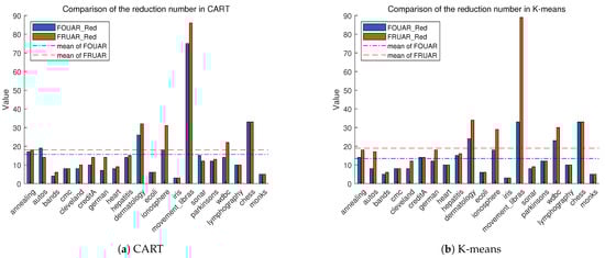
Figure 1.
Reduction Number Comparison.
From the figures, we can conclude that FOUAR has a stronger capability to remove redundant attributes compared to the traditional attribute reduction algorithm. Given that FOUAR generally performs better in downstream tasks, we deduce that FOUAR is more suitable for reduction experiments where the downstream tasks are classification and clustering.
6.6. Parameter Experiment
In this subsection, we conduct a parameter experiment analysis. In FOUAR, serves as a critical adjustable parameter, enabling the control of the granularity of fuzzy-rough data analysis. As a result, FOUAR can fine-tune the reduced attribute subset of the dataset by adjusting , allowing the reduced dataset to achieve good performance in various learning algorithms. We showcase the graphs of the accuracy of learning algorithms and the number of reduced attributes as functions of in Figure 2, highlighting FOUAR’s reduction capabilities and its ability to preserve data features. It should be noted that the number of reduced attributes equals the total attributes in the dataset minus the attributes retained after reduction.
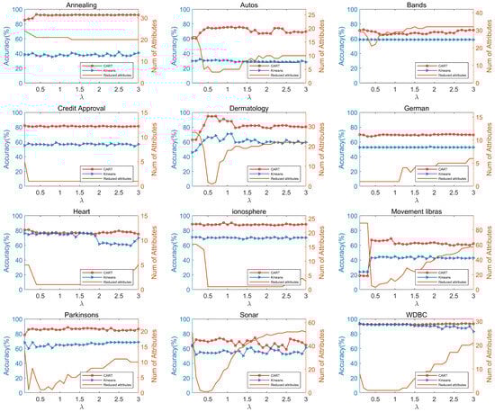
Figure 2.
Parameter Experiment.
From Figure 2, we observe that, in most datasets, the number of reduced attributes initially decreases rapidly as changes, then gradually increases until stabilizing, as exemplified in the Bands, Autos, Dermatology, Movement libras, Parkinsons, Sonar, and WDBC datasets. For the Annealing and German datasets, the number of reduced attributes remains stable or slowly increases, respectively. However, for the Credit Approve and Ionosphere datasets, the number of reduced attributes initially decreases and remains stable without further increases, while for the Heart dataset, the number of reduced attributes begins to gradually increase after a prolonged period of relatively low reduction. Based on this analysis of the number of reduced attributes, we find that FOUAR achieves more significant reduction effects when has a larger value. This is because a larger results in smaller granularity of fuzzy-rough data, leading to a more accurate approximation of the target set. Consequently, the dependencies between attributes can be better expressed.
For most datasets in Figure 2, the classification and clustering accuracies remain within a relatively stable range. However, for the Dermatology dataset, the classification and clustering accuracies are initially unstable, becoming stable only when exceeds . Analyzing the changes in classification and clustering accuracies with respect to , we observe that FOUAR is not sensitive to changes in when processing most datasets, enabling FOUAR to stably maintain data characteristics.
In summary, the experimental analysis demonstrates that FOUAR exhibits outstanding performance in terms of reduction efficiency and preservation of data features.
6.7. Hypothesis Testing
In this section, we report hypothesis testing experiments on FOUAR using prediction accuracy and clustering accuracy data obtained from classification and clustering experiments. The Friedman test [48] and Nemenyi test [49] were used for this purpose.
Before conducting the Friedman test, we first need to rank the accuracies of each algorithm on different datasets in ascending order and assign natural numbers to these sorted accuracies, referred to as ranks. If there are ties in accuracy, we need to equally distribute these ranks among the tied values.
Suppose we need to compare M algorithms on N datasets, where represents the average rank of all corresponding accuracies for each participating algorithm. The Friedman test can be calculated as:
However, the original Friedman test statistic is too conservative, so a new statistic, , is introduced:
where follows an F-distribution with degrees of freedom and . The null hypothesis of the Friedman test is that ‘there is no significant difference among all algorithms in terms of their performance on the datasets’. Thus, if the null hypothesis is rejected, it indicates significant differences among the algorithms. To further differentiate the differences between the algorithms, we conducted post hoc tests. The Nemenyi test, as a widely used post hoc test, was adopted in this paper. Its core purpose is to compare the differences between algorithms with a critical difference. By calculating the critical difference, significant differences at the confidence level can be obtained. In the Nemenyi test, the critical difference (CD) is calculated by the formula:
where is the critical value obtained from the table based on the significance level , which can be found in [49]. If the difference between algorithms is greater than the average rank difference, it indicates a significant difference between them.
In hypothesis-testing experiments, we obtained and in the Friedman test with a significance level of . The degrees of freedom for were 5 and 105. We obtained a critical value of for each learning algorithm in the Friedman test, and, if was greater than the critical value, we rejected the null hypothesis of no significant difference between the algorithms.
In the case of CART, , while for KNN and K-means, and , respectively. As all of the values exceed the critical value, the null hypothesis was rejected for all algorithms in the Friedman test, indicating a significant difference among them. Further hypothesis testing was performed using the Nemenyi test, and the results are presented in Figure 3.
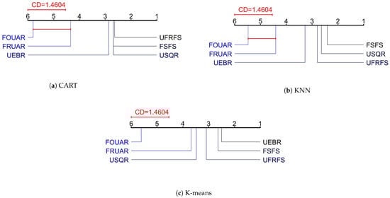
Figure 3.
Post hoc test.
Based on the results shown in Figure 3a, it is apparent that FOUAR exhibits significant differences when compared to most of the other reduction algorithms. In Figure 3c, significant differences were observed between FOUAR and FRUAR, USQR, UEBR, FSFS, and UFRFS. Additionally, FOUAR had the highest average rank among all the reduction algorithms in (a), (b) and (c). These findings suggest that FOUAR is a superior attribute reduction algorithm in comparison to the other methods tested, making it a suitable choice for learning tasks such as classification and clustering.
7. Conclusions
This paper proposes an unsupervised attribute reduction algorithm for mixed data based on an improved optimal approximation set. First, we propose the theory of an improved optimal approximation set along with its corresponding algorithm, named IOAS. Then, we broaden the classical optimal approximation set theory to encompass fuzzy set theory, leading to the creation of a fuzzy improved optimal approximation set algorithm (FIOAS). Lastly, in order to leverage the information of the upper approximation set, we propose an attribute significance function and a relevance function based on the fuzzy optimal approximation set, culminating in the development of an unsupervised attribute reduction algorithm (FOUAR).
To evaluate the effectiveness of FOUAR and IOAS, 22 datasets from the UCI database were selected for experiments. The results indicate that the improved algorithm for computing the optimal approximation set achieves higher approximation accuracy and smaller approximation set volume. Furthermore, FOUAR maintains or even improves the prediction and clustering accuracy of the reduced dataset and outperforms existing unsupervised attribute reduction algorithms.
In future work, the proposed fuzzy optimal approximation-based reduction algorithm will be extended to supervised positive region reduction algorithms. Additionally, algorithms will be designed to obtain globally optimal reduced attributes.
Author Contributions
Methodology, H.W.; Writing—original draft, H.W.; Writing—review and editing, H.W., S.Z. and M.L. All authors have read and agreed to the published version of the manuscript.
Funding
This research was funded by the National Natural Science Foundation of China (No. 72101082), and the Natural Science Foundation of Hebei Province (No. A2020208004). The APC was funded by the National Natural Science Foundation of China (No. 72101082), and the Natural Science Foundation of Hebei Province (No. A2020208004).
Data Availability Statement
Simulation datasets supporting reported results can be found at the link to the publicly archived UCI Machine Learning Repository http://archive.ics.uci.edu/ml (accessed on 30 March 2022).
Conflicts of Interest
The authors declare no conflict of interest.
References
- Pawlak, Z. Rough sets. Int. J. Parallel. Prog. 1982, 11, 341–356. [Google Scholar] [CrossRef]
- Ma, X.-A.; Xu, H.; Ju, C. Class-specific feature selection via maximal dynamic correlation change and minimal redundancy. Expert Syst. Appl. 2023, 229, 120455. [Google Scholar] [CrossRef]
- Zhang, X.; Yao, Y. Tri-level attribute reduction in rough set theory. Expert Syst. Appl. 2022, 190, 116187. [Google Scholar] [CrossRef]
- Yao, Y.; Zhang, X. Class-specific attribute reducts in rough set theory. Inform. Sci. 2017, 418–419, 601–618. [Google Scholar] [CrossRef]
- Dong, L.J.; Chen, D.G.; Wang, N.; Lu, Z.H. Key energy-consumption feature selection of thermal power systems based on robust attribute reduction with rough sets. Inf. Sci. 2020, 532, 61–71. [Google Scholar]
- Zhang, P.F.; Li, T.R.; Wang, G.Q.; Luo, C.; Chen, H.M.; Zhang, J.B.; Wang, D.X.; Yu, Z. Multi-source information fusion based on rough set theory: A review. Inform. Fusion 2021, 68, 85–117. [Google Scholar] [CrossRef]
- Zhang, X.Y.; Yao, H.; Lv, Z.Y.; Miao, D.Q. Class-specific information measures and attribute reducts for hierarchy and systematicness. Inf. Sci. 2021, 563, 196–225. [Google Scholar] [CrossRef]
- Lashin, M.M.A.; Khan, M.I.; Khedher, N.B.; Eldin, S.M. Optimization of Display Window Design for Females’ Clothes for Fashion Stores through Artificial Intelligence and Fuzzy System. Appl. Sci. 2022, 12, 11594. [Google Scholar] [CrossRef]
- Kouatli, I. The Use of Fuzzy Logic as Augmentation to Quantitative Analysis to Unleash Knowledge of Participants’ Uncertainty When Filling a Survey: Case of Cloud Computing. IEEE Trans. Knowl. Data Eng. 2022, 34, 1489–1500. [Google Scholar] [CrossRef]
- Dubois, D.; Prade, H. Rough fuzzy sets and fuzzy rough sets. Int. J. Gen. Syst. 1990, 17, 191–209. [Google Scholar] [CrossRef]
- Dubois, D.; Prade, H. Putting rough sets and fuzzy sets together. In Intelligent Decision Support; Springer: Berlin/Heidelberg, Germany, 1992; pp. 203–232. [Google Scholar]
- Sun, B.Z.; Ma, W.M.; Qian, Y.H. Multigranulation fuzzy rough set over two universes and its application to decision making. Knowl.-Based Syst. 2017, 123, 61–74. [Google Scholar] [CrossRef]
- Morsi, N.N.; Yakout, M.M. Axiomatics for fuzzy rough sets. Fuzzy Sets Syst. 1998, 100, 327–342. [Google Scholar] [CrossRef]
- Moser, B. On the T-transitivity of kernels. Fuzzy Sets Syst. 2006, 157, 1787–1796. [Google Scholar] [CrossRef]
- Jensen, R.; Shen, Q. Fuzzy–rough attribute reduction with application to web categorization. Fuzzy Sets Syst. 2004, 141, 469–485. [Google Scholar] [CrossRef]
- Hu, Q.H.; Xie, Z.X.; Yu, D.R. Hybrid attribute reduction based on a novel fuzzy-rough model and information granulation. Pattern Recogn. 2007, 40, 3509–3521. [Google Scholar] [CrossRef]
- Wang, C.Z.; Huang, Y.; Shao, M.W.; Fan, X.D. Fuzzy rough set-based attribute reduction using distance measures. Knowl.-Based Syst. 2019, 164, 205–212. [Google Scholar] [CrossRef]
- Ganivada, A.; Ray, S.S.; Pal, S.K. Fuzzy rough sets, and a granular neural network for unsupervised feature selection. Neural Netw. 2013, 48, 91–108. [Google Scholar] [CrossRef]
- Mac Parthaláin, N.; Jensen, R. Unsupervised fuzzy-rough set-based dimensionality reduction. Inf. Sci. 2013, 229, 106–121. [Google Scholar] [CrossRef]
- Yuan, Z.; Chen, H.; Li, T.; Yu, Z.; Sang, B.; Luo, C. Unsupervised attribute reduction for mixed data based on fuzzy rough sets. Inf. Sci. 2021, 572, 67–87. [Google Scholar] [CrossRef]
- Hu, M.; Guo, Y.; Chen, D.; Tsang, E.C.C.; Zhang, Q. Attribute reduction based on neighborhood constrained fuzzy rough sets. Knowl.-Based Syst. 2023, 274, 110632. [Google Scholar] [CrossRef]
- Dai, J.; Wang, Z.; Huang, W. Interval-valued fuzzy discernibility pair approach for attribute reduction in incomplete interval-valued information systems. Inf. Sci. 2023, 642, 119215. [Google Scholar] [CrossRef]
- Wang, P.; He, J.; Li, Z. Attribute reduction for hybrid data based on fuzzy rough iterative computation model. Inf. Sci. 2023, 632, 555–575. [Google Scholar] [CrossRef]
- Qu, L.; He, J.; Zhang, G.; Xie, N. Entropy measure for a fuzzy relation and its application in attribute reduction for heterogeneous data. Appl. Soft Comput. 2022, 118, 108455. [Google Scholar] [CrossRef]
- Zhai, Y.; Li, D. Knowledge structure preserving fuzzy attribute reduction in fuzzy formal context. Int. J. Approx. Reason. 2019, 115, 209–220. [Google Scholar] [CrossRef]
- Yang, S.; Zhang, H.; Shi, G.; Zhang, Y. Attribute reductions of quantitative dominance-based neighborhood rough sets with A-stochastic transitivity of fuzzy preference relations. Appl. Soft Comput. 2023, 134, 109994. [Google Scholar] [CrossRef]
- Guo, Y.; Hu, M.; Wang, X.; Tsang, E.C.C.; Chen, D.; Xu, W. A robust approach to attribute reduction based on double fuzzy consistency measure. Knowl.-Based Syst. 2022, 253, 109585. [Google Scholar] [CrossRef]
- Ziarko, W. Variable precision rough set model. J. Comput. Syst. Sci. 1993, 46, 39–59, ISSN 0022-0000. [Google Scholar] [CrossRef]
- Chen, J.; Zhu, P. A variable precision multigranulation rough set model and attribute reduction. Soft Comput. 2023, 27, 85–106. [Google Scholar] [CrossRef]
- Dai, J.H.; Han, H.F.; Zhang, X.H.; Liu, M.F.; Wan, S.P.; Liu, J.; Lu, Z.L. Catoptrical rough set model on two universes using granule-based definition and its variable precision extensions. Inf. Sci. 2017, 390, 70–81. [Google Scholar] [CrossRef]
- Li, R.; Wang, Q.H.; Gao, X.F.; Wang, Z.J. Research on fuzzy order variable precision rough set over two universes and its uncertainty measures. Proc. Comput. Sci. 2019, 154, 283–292. [Google Scholar] [CrossRef]
- Zhang, Q.H.; Wang, G.Y.; Xiao, Y. Approximation sets of rough sets. J. Softw. 2012, 23, 1745–1759. [Google Scholar] [CrossRef]
- Zhang, Q.H.; Xue, Y.B.; Hu, F.; Yu, H. Research on Uncertainty of Approximation Set of Rough Set. Acta Electron. Sin. 2016, 44, 1574. [Google Scholar]
- Zhang, Q.H.; Xue, Y.B.; Wang, G.Y. Optimal approximation sets of rough sets. J. Softw. 2016, 27, 295–308. [Google Scholar]
- Luo, L.P.; Liu, E.G.; Fan, Z.Z. Optimal Approximation Rough Set. J. Henan Univ. Sci. Technol. Sci. 2018, 39, 89–93. [Google Scholar]
- Luo, L.P.; Liu, E.G.; Fan, Z.Z. Attributes reduction based on optimal approximation set of rough set. Appl. Res. Comput. 2019, 36, 1940–1942. [Google Scholar]
- Luo, L.P.; Liu, E.G.; Fan, Z.Z. Matrix Computation for Optimal Approximation Rough Set. J. East China Jiaotong Univ. 2018, 35, 83–88. [Google Scholar]
- Yuan, J.X.; Zhang, W.X. The Inclusion Degree and Similarity Degree of Fuzzy Rough Sets. Fuzzy Syst. Math. 2005, 1, 111–115. [Google Scholar]
- Yeung, D.S.; Chen, D.G.; Tsang, E.C.C.; Lee, J.W.T.; Wang, X.Z. On the generalization of fuzzy rough sets. IEEE Trans. Fuzzy Syst. 2005, 13, 343–361. [Google Scholar] [CrossRef]
- Yuan, Z.; Zhang, X.Y.; Feng, S. Hybrid data-driven outlier detection based on neighborhood information entropy and its developmental measures. Expert Syst. Appl. 2018, 112, 243–257. [Google Scholar] [CrossRef]
- Dheeru, D.; Taniskidou Karra, E. UCI Machine Learning Repository. 2017. Available online: http://archive.ics.uci.edu/ml (accessed on 30 March 2022).
- Zhu, P.F.; Zhu, W.C.; Hu, Q.H.; Zhang, C.Q.; Zuo, W.M. Subspace clustering guided unsupervised feature selection. Pattern Recogn. 2017, 66, 364–374. [Google Scholar] [CrossRef]
- Mitra, P.; Murthy, C.; Pal, S.K. Unsupervised feature selection using feature similarity. IEEE Trans. Pattern Anal. Mach. Intell. 2002, 24, 301–312. [Google Scholar] [CrossRef]
- Velayutham, C.; Thangavel, K. Unsupervised quick reduct algorithm using rough set theory. J. Electron. Sci. Technol. 2011, 9, 193–201. [Google Scholar]
- Velayutham, C.; Thangavel, K. A novel entropy based unsupervised feature selection algorithm using rough set theory. In Proceedings of the IEEE-International Conference on Advances in Engineering, Science and Management (ICAESM-2012), Nagapattinam, India, 30–31 March 2012; IEEE: Manhattan, NY, USA, 2012; pp. 156–161. [Google Scholar]
- Hu, Q.H.; Yu, D.R.; Xie, Z.X. Information-preserving hybrid data reduction based on fuzzy-rough techniques. Pattern Recogn. Lett. 2006, 27, 414–423. [Google Scholar] [CrossRef]
- Yu, D.R.; Hu, Q.H.; Bao, W. Combining rough set methodology and fuzzy clustering for knowledge discovery from quantitative data. Proc. CSEE 2004, 24, 205–210. [Google Scholar]
- Friedman, M. A comparison of alternative tests of significance for the problem of m rankings. Ann. Math. Stat. 1940, 11, 86–92. [Google Scholar] [CrossRef]
- Demšar, J. Statistical comparisons of classifiers over multiple datasets. J. Mach. Learn. Res. 2006, 7, 1–30. [Google Scholar]


Disclaimer/Publisher’s Note: The statements, opinions and data contained in all publications are solely those of the individual author(s) and contributor(s) and not of MDPI and/or the editor(s). MDPI and/or the editor(s) disclaim responsibility for any injury to people or property resulting from any ideas, methods, instructions or products referred to in the content. |
© 2023 by the authors. Licensee MDPI, Basel, Switzerland. This article is an open access article distributed under the terms and conditions of the Creative Commons Attribution (CC BY) license (https://creativecommons.org/licenses/by/4.0/).