Two-Step Adaptive Control for Planar Type Docking of Autonomous Underwater Vehicle

Abstract

Planar type docking enables a convenient underwater energy supply for irregularly shaped autonomous underwater vehicles (AUVs), but the corresponding control method is still challenging. Conventional control methods for torpedo-shaped AUVs are not suitable for planar type docking due to the significant differences in system structures and motion characteristics. This paper proposes a two-step adaptive control method to solve the planar type docking problem. The method makes a seamless combination of horizontal dynamic positioning and visual servo docking considering ocean current disturbance. The current disturbance is estimated and canceled in the pre-docking step using a current observer, and the positioning error is further compensated for by the vertical visual servo technique in the docking step. Reduced order dynamic models are distinctively established for different docking steps according to the motion characteristics, based on which the dynamic controllers are designed considering the model parameter uncertainties. Simulation is conducted with an initial distance of 10 m in the horizontal direction and 3 m in depth. Stable and accurate dynamic positioning under up to 0.4 m/s of current disturbances with different directions is validated. A 0.5 m lateral positioning error is successfully compensated for by the visual servo docking step. The proposed control method provides a valuable reference for similar types of docking application.

1. Introduction

Autonomous underwater vehicles (AUVs) play an important role in ocean explorations [1,2,3], but their working durations are often limited by their battery capacities [4]. Underwater docking based on seabed stations is a feasible solution for unmanned charging and data collections [5,6,7]. However, conventional docking stations are usually tailored for specific types of AUVs, and are hardly capable for other shapes and structures. For example, the most popular cone-shaped docking stations are usually customized for torpedo-shaped AUVs [8,9].

As there is an increasing need for executing complex tasks, the shapes and structures of AUVs are diversified for extended functions [10]. In many occasions, irregularly shaped AUVs are more preferred for close-range and high-resolution underwater observation tasks than conventional torpedo-shaped AUVs [11,12], but the corresponding docking system designs are still challenging. Most of the current irregularly shaped docking systems have complex connecting and fitting structures along with complicated docking control methods [13,14], and thus are difficult to be further extended to other system constructions.

Aiming at providing a generalized solution for unconventional shaped AUVs, an omnidirectional positioning-tolerant planar type AUV docking and charging system was developed in our previous work [15]. The concise planar docking surface is widely capable for various kinds of AUVs with complex shapes and structures. Our previous work conducted a preliminary exploration on the system construction, and this paper conducts deeper research on the docking control method in the presence of ocean current disturbance and model parameter uncertainties.

Although AUV docking control methods have been actively studied in the past decades, rare attempts have been made to solve the planar docking problems. Conventional docking control studies mainly focus on the torpedo-shaped AUVs with cone-shaped docking stations [16,17]. The control schemes can be divided into homing and docking steps, where the heading control of the AUVs is of the highest priority [18,19,20]. However, the control scheme for the planar type docking system is very different. The AUV usually performs horizontal navigations, but the terminal identification of the docking platform relies on the downward looking camera. As an extension of our previous work [15], this paper investigates a two-step planar docking controller that combines horizontal dynamic positioning with vertical visual servo docking, which is substantially different from the conventional docking method for the torpedo-shaped AUVs.

Dynamic positioning is a typical control problem that has been widely discussed in the literature [21,22,23,24,25,26]. A non-linear adaptive controller is proposed in [21] to address the dynamic positioning and way-point tracking problem, and lays a solid foundation in the field. The research in [22] investigated a robust hybrid control method considering perturbations due to ocean currents, and only leaving out model uncertainties as future research. Advanced dynamic control strategies such as the network-based Takagi–Sugeno fuzzy control in [23] and the model predictive and neural networks in [24] have a satisfying performance and deal well with external disturbance, but also suffer from a high computational cost. Other methods including the sliding mode control [25] and backstepping control [26] are also validated, but the application scenarios need to be further expanded. In addition, present work tends to treat the dynamic positioning as an independent problem. The cooperation with other tasks, especially the planar type docking, has rarely been discussed. In addition, there is still a gap between the theoretical method and the applications on real systems, especially for the low-cost miniaturized AUVs where sensors and computational capabilities are limited.

Visual servo is another essential technique involved in the proposed method [27]. Specifically, monocular vision is an efficient and cost-effective approach to achieve the stabilization of an AUV in front of a planar target [28]. Typical examples of the visual servo of fully actuated AUVs include the inertial-aided visual servo approach investigated in [12,29], the sliding-mode observer-based model predictive control proposed in [30] and the pipeline following application conducted in [11]. However, these methods have not yet been extended to underactuated underwater AUVs. An extreme learning-based monocular visual servo is developed for unmanned surface vessel in [31]. An adaptive neural network is applied in a hierarchical model predictive visual servo in [32]. These comprehensive algorithms are proven to have a promising performance, but also increase the computational burdens. In addition, the control target for most visual servo methods are static target poses, and the dynamic approaching process during docking has rarely been studied. There is also a lack of an integrated method containing dynamic visual servo to solve the planar docking problem.

Despite the existing studies on the underwater dynamic positioning and visual servo issues, to the best of our knowledge, making seamless combination of these two methods to solve the planar docking problem in the presence of environment disturbances and model uncertainties is still challenging. In this paper, a two-step adaptive planar type docking controller is investigated. The main contributions are highlighted as follows:

• The two-step docking method takes full advantage of the omnidirectional feature of the planar type docking station. A seamless combination of dynamic positioning and three-dimensional (3D) visual servo is made to achieve a stable and accurate docking control.
• The controller perfectly matches up with the underactuated feature of the prototype AUV, where a roll motion adjustment is adopted to rapidly compensate for the visual error and gradually reduce the actual positioning error during the descending docking process.
• Practical issues are fully considered in the controller design and simulation validation, including hardware limitations, unknown ocean current disturbance, inevitable positioning error and model parameter uncertainties.

The rest of this paper is organized as follows: Section 2 introduces the concept of planar type docking for a HOME-I AUV, and establishes kinematic and dynamic models. In Section 3, the two-step control strategy is introduced and the model-based controllers are designed. Section 4 presents the simulation results together with the analysis. Section 5 concludes the paper.

2. Problem Statement

2.1. Planar Type Docking Task

The planar type docking control problem is investigated based on the miniaturized HOME-I AUV and the planar type docking and charging station developed in our previous work [15]. The system outline and the docking process is briefly illustrated in Figure 1. The underactuated AUV is capable of a 4 degrees of freedom (DOFs) motion. It has a downward looking camera to recognize the subsea terrain and the platform surface. The platform surface has a concise planar docking and charging board. This structure naturally has no constraints on the AUV structure and provides large positioning tolerance for docking. A distinctive pattern is painted on the platform surface, which can be recognized by the AUV camera. All the circuit components are sealed inside a pressure chamber under the charging board.

The general docking strategy is designed according to the features of the docking system. Given that the docking task target is to land the AUV on the platform surface, the docking process is intuitively divided into two steps as illustrated in Figure 1.

• Pre-docking horizontal dynamic positioning step. The AUV returns to the station at a constant depth and dynamically stops on the top of the platform. In the presence of an ocean current, it aligns itself in an antiparallel direction with the current so that the disturbance can be easily canceled by the surge motion.
• Vertical visual servo landing and docking step. The AUV descends and lands on the platform center using a 3D visual servo strategy. Since the docking station allows an arbitrary landing direction of the AUV, the heading angle of the AUV merely depends on the current direction, which brings much convivence and stability of the docking process.

This paper aims at developing an integrated controller combining the two steps as stated above. Practical issues such as unknown ocean current disturbance, inevitable positioning error and model parameter uncertainties are all considered.

2.2. Kinematic Model

The kinematic model of the HOME-I AUV is established in a global north east down coordinate frame (NED frame) and a body-fixed coordinate frame (B-frame), as illustrated in Figure 2. For the docking task in a small area, assuming a constant current disturbance $v_w={[v_{wx}, v_{wy}, 0, 0, 0, 0]}^{\mathrm{T}}$ on the x and y direction in the NED frame, and the AUV velocity in the B-frame $v_r^b={[u_r, v_r, w, p, q, r]}^{\mathrm{T}}$ independent of the current velocity v_w. Unless otherwise stated, the AUV velocities in this paper all denote the velocities in the B-frame.

In the pre-docking step, the AUV mainly performs a horizontal motion so that it is self-stabilized in the pitch and roll motion. It conducts a decoupled 3-DOF motion on the horizontal plane along with an independently controlled depth, which gives a simplified kinematic model according to T.I Fossen [33]:

$$\begin{array}{l}\dot{x}=u_r\cos \psi -v_r\sin \psi +v_{wx},\\ \dot{y}=u_r\sin \psi +v_r\cos \psi +v_{wy},\\ \dot{\psi }=r,\\ \dot{z}=w.\end{array}$$

(1)

For the convenience of the kinematic controller design, let P_d(x_d, y_d) be a target point right above the center of the docking plane, $\epsilon$ be the distance between the current position P and P_d and γ be the angle measured from the current heading direction to the direction of P_d. A coordinate transformation inspired from [21] is applied as shown in Figure 2b and calculated in (2).

$$\begin{array}{l}\epsilon ={\left({(x-x_d)}^2+{(y-y_d)}^2\right)}^{1/2},\\ \gamma =\arctan \left(\frac{y_d-y}{x_d-x}\right)-\psi ,\end{array}$$

(2)

The error dynamics of (2) is written as:

$$\begin{array}{l}\dot{\epsilon }=-u_r\cos \gamma -v_r\sin \gamma -V_w\cos (\psi +\gamma -{\psi }_w),\\ \dot{\gamma }=\left[u_r\sin \gamma -v_r\cos \gamma +V_w\sin (\psi +\gamma -{\psi }_w)\right]{\epsilon }^{-1}-r, \epsilon \ne 0,\\ \dot{\psi }=r,\end{array}$$

(3)

where $V_w=\sqrt{v_{wx}^2+v_{wy}^2}$ and ${\psi }_w=\mathit{atan}2(v_{wy},v_{wx})$.

The docking step is performed when the docking platform is recognized by the AUV camera. Compared to the pre-docking process in a longer range, the terminal docking process needs a more accurate and faster control to land the AUV precisely on the docking platform. Therefore, a visual servo controller is adopted during the docking process. Instead of using the position in the NED frame, the controller takes the docking platform pattern as a reference and directly takes the visual errors as feedback to provide reference velocities in the kinematic level. The design concept is straightforward. Complex coordinate transformation and redundant calculations are avoided. The visual servo schematic is illustrated in Figure 3.

In Figure 3, the position of the platform center in the NED frame is P_c, the norm vector is n_r. F_r and F denote the reference and current camera coordinate frames, respectively. R and t are the rotation matrix and translation vector from the current frame F to the reference frame F_r, respectively. The position of P_c is P_r in the frame F_r and P in the frame F. Referring to our previous work [15], a visual objective function is defined as:

$$e=\left[\begin{array}{c}{e}_v\\ e_{\omega }\end{array}\right]=\left[\begin{array}{c}-t+(I-R)P_r\\ -2\alpha \sin \xi -S(n_r)t\end{array}\right],$$

(4)

where the rotation matrix R is also denoted by a rotation angle ξ along a unit vector axis α. S(a) denotes the antisymmetric matrix of a vector a = (a₁, a₂, a₃) given by (5).

$$S(a)=\left[\begin{array}{ccc}0& -a_3& a_2\\ a_3& 0& -a_1\\ -a_2& a_1& 0\end{array}\right].$$

(5)

From the perspective of computer vision, the objective function can also be written as:

$$e=\left[\begin{array}{c}{e}_v\\ e_{\omega }\end{array}\right]=\left[\begin{array}{c}\left(I-H\right)P_r\\ S^{-1}(H^{\mathrm{T}}-H)\end{array}\right],$$

(6)

where H is the homography matrix from F_r to F, which can be easily obtained by the image processing technique. S⁻¹ denotes the inverse operation of S. The expressions in (6) and (4) are isomorphic, which means that e = 0 only when ω = 0 and t = 0.

The time derivative of the objective function (4) is:

$$\dot{e}=\left[\begin{array}{c}{\dot{e}}_v\\ {\dot{e}}_{\omega }\end{array}\right]=\left[\begin{array}{cc}I& S(-e_v+P_r)\\ S(n_r)& -S(n_r)S(t)+2\Omega \end{array}\right]\left[\begin{array}{c}v\\ \omega \end{array}\right],$$

(7)

where:

$$\Omega =I-\frac{\sin \xi }{2}S(\alpha )-{\sin }^2\left(\frac{\xi }{2}\right)\left(2{\rm I}+S^2(\alpha )\right),$$

(8)

$v={[u_r+u_w, v_r+v_w, w]}^{\mathrm{T}}$ and $\omega ={[p, q, r]}^{\mathrm{T}}$ are the overall translational and rotational velocities in the B-frame. u_w and v_w are the current velocities in the surge and sway directions.

As introduced above, the charging platform gives no constraint on the heading direction of the AUV. Moreover, when constant ocean current disturbance exists, the AUV must be kept aligned with the water flow direction for stability concerns during the descending process. Therefore, instead of letting the whole objective function asymptotically converge to zero, only the translation component of $\dot{e}$ is considered here as:

$${\dot{e}}_v=v+S(-e_v+P_r)\omega .$$

(9)

Expanding (9) yields:

$${\dot{e}}_v=\left[\begin{array}{c}{\dot{e}}_u\\ \begin{array}{l}{\dot{e}}_v\\ {\dot{e}}_w\end{array}\end{array}\right]=\left[\begin{array}{l}(u_r+u_w)+(-e_w+Z_r)q-(-e_v+Y_r)r\hfill \\ (v_r+v_w)-(-e_w+Z_r)p+(-e_u+X_r)r\hfill \\ w+(-e_v+Y_r)p-(-e_u+X_r)q\hfill \end{array}\right],$$

(10)

where $e_v=\left[e_u, e_v, e_w\right]$, $P_r=\left[X_r, Y_r, Z_r\right]$, and the antisymmetric matrix operator S is given in (5). Since the visual servo controller is designed based on (10) and provides reference velocities in the kinematic level, Equation (10) is equivalent to a kinematic model, but is in a more straightforward manner for the visual servo controller design.

2.3. Dynamic Model

The simplified dynamics in the two steps are acquired from the 6-DOF dynamic model given by:

$$M{\dot{v}}_r+C(v_r)v_r+D(v_r)v_r+G(\eta )\eta =\tau ,$$

(11)

where M, C, D, and G are the mass, Coriolis-centripetal, viscous damping and restoring force terms, respectively. During the pre-docking process, the pitch and roll motion are self-stabilized so that the 6-DOF dynamics can be simplified into decoupled 3-DOF dynamics. The high order terms and nonlinear terms in the viscous hydrodynamic force can also be neglected during the low-speed docking motion. Therefore, the dynamics are given by:

$$\begin{array}{l}{m}_u{\dot{u}}_r-m_v{v}_{r}r+d_u{u}_r={\tau }_u,\\ m_v{\dot{v}}_r+m_u{u}_{r}r+d_v{v}_r=0,\\ m_r{\dot{v}}_r-m_{uv}{u}_r{v}_r+d_r{v}_r={\tau }_r.\end{array}$$

(12)

where $m_u=m-X_{\dot{u}}$, $m_v=m-Y_{\dot{v}}$, $m_r=I_z-N_{\dot{r}}$, $m_{uv}=m_u-m_v$.

During the visual servo docking step, the roll motion is actively adjusted, which gives a set of 4-DOF dynamics as:

$$\begin{array}{l}{m}_u{\dot{u}}_r+d_u{u}_r={\tau }_u,\\ m_v{\dot{v}}_r-m{z}_g\dot{p}-m_{w}wp+d_v{v}_r=0,\\ m_w\dot{w}+m_v{v}_{r}p+d_{w}w-m{z}_g{p}^2={\tau }_w,\\ m_p\dot{p}-m_{vw}{v}_{r}w+d_{p}p-m{z}_{g}pw+m{z}_{g}g\sin \varphi ={\tau }_p.\end{array}$$

(13)

where $m_u=m-X_{\dot{u}}$, $m_v=m-Y_{\dot{v}}$$m_w=m-Z_{\dot{w}}$, $m_p=I_x-K_{\dot{p}}$, $m_{vw}=m_v-m_w$ and the position of the center of gravity is (0, 0, z_g) in the B-frame. Notice that the AUV is underactuated in its sway motion. The dynamic controller in each docking step is then designed based on the dynamic models described by (12) or (13).

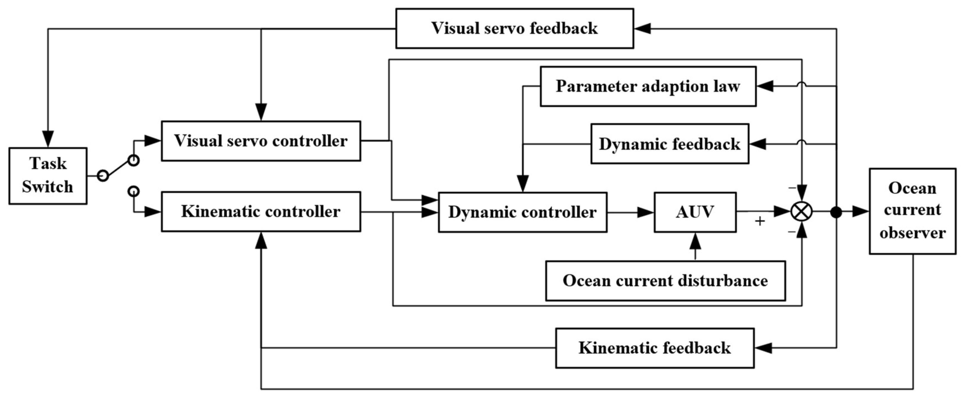
3. Controller Design

Following the two-step docking strategy introduced in Section 2, a control diagram is established as illustrated in Figure 4. The controller contains two closed loops. A kinematic controller in the outer loop is applied for the pre-docking dynamic positioning step. An ocean current observer is utilized to deal with the current disturbance. For the docking step, the outer loop controller is switched to the visual servo controller, which directly takes the visual errors of the platform pattern as feedback. The task is switched according to whether the docking platform is caught sight of and recognized by the AUV camera.

The dynamic controllers in the inner loop of the two steps are designed based on different decoupled dynamic models in (12) and (13) but following a similar design methodology. A parameter adaption law is applied to deal with the model parameter uncertainties. Detailed control algorithms are introduced in the later subsections.

3.1. Pre-Docking Step

According to the kinematic model in (3) and referring to the method introduced in [21], the kinematic controller is chosen as:

$$\begin{array}{l}{u}_r=k_u\epsilon -V_w\cos (\psi -{\psi }_w),\\ r=k_r\gamma +k_u\sin \gamma -{\epsilon }^{-1}{v}_r\cos \gamma +{\epsilon }^{-1}{V}_w\sin (\psi -{\psi }_w)\cos \gamma ,\epsilon \ne 0.\end{array}$$

(14)

Considering the Lyapunov function $V_{k\gamma }(\gamma )=\frac{1}{2}{\gamma }^2$, applying the controller in (14), the time derivative of $V_{k\gamma }(\gamma )$ is:

$$\begin{array}{l}{\dot{V}}_{k\gamma }(\gamma )=-\gamma \left[\left(u_r\sin \gamma -v_r\cos \gamma +V_w\sin (\psi +\gamma -{\psi }_w)\right){\epsilon }^{-1}-r\right]\\ \hspace{1em}\hspace{1em}\hspace{1em} =-k_r{\gamma }^2<0.\end{array}$$

(15)

Therefore, γ is bounded and exponentially converges to zero as $t\to \infty$. Then considering the Lyapunov function $V_{k\epsilon }(\epsilon )=\frac{1}{2}{\epsilon }^2$, the time derivative of $V_{k\epsilon }(\epsilon )$ is given by:

$${\dot{V}}_{k\epsilon }(\epsilon )=-k_u\cos \gamma {\epsilon }^2+\beta \epsilon ,$$

(16)

where:

$$\beta =V_w[(\cos (\psi -{\psi }_w)\cos \gamma -\cos (\psi +\gamma -{\psi }_w)]-v_r\sin \gamma .$$

(17)

Since γ, V_w and v_r are bounded and γ converges to zero as $t\to \infty$, β converges to zero as $t\to \infty$. Moreover, there exists a finite time t₀ > 0 and γ₀ such that γ < γ₀ when t > t₀. Therefore, (16) becomes:

$$\begin{array}{ll}{\dot{V}}_{k\epsilon }(\epsilon )& \le -k_u\cos {\gamma }_0{\epsilon }^2+\beta \epsilon \hspace{1em} \forall t>t_0\\ & =-k_u\cos {\gamma }_0{\epsilon }^2(1-\sigma )-\sigma k_u\cos {\gamma }_0{\epsilon }^2+\beta \epsilon , 0\le \sigma <1\\ & \le -k_u\cos {\gamma }_0{\epsilon }^2(1-\sigma )<0, \forall \left|\epsilon \right|\ge \left|\beta \right|{\left(\sigma k_u\cos {\gamma }_0\right)}^{-1}.\end{array}$$

(18)

which indicates that $\epsilon$ is bounded and converges to zero as $t\to \infty$.

For an unknown but constant current disturbance, an observer is designed as:

$$\begin{array}{l}\dot{\widehat{x}}=u_r\cos \psi -v_r\sin \psi +{\widehat{v}}_{wx}+k_{ox1}\tilde{x},\\ \dot{\widehat{y}}=u_r\sin \psi +v_r\cos \psi +{\widehat{v}}_{wy}+k_{oy1}\tilde{y},\\ {\widehat{v}}_{wx}=k_{ox2}\tilde{x},\\ {\widehat{v}}_{wy}=k_{oy2}\tilde{x},\end{array}$$

(19)

where $\widehat{•}$ denotes the estimation parameters, $\tilde{x}=x-\widehat{x}$ and $\tilde{y}=y-\widehat{y}$. The following lemma is then established.

Lemma 1.

Assuming the ocean current disturbance is constant but unknown. Considering the observer in (19), where the positive gains k_ox1, k_ox2, k_oy1 and k_oy2 are chosen such that the observer asymptotically stable. The current (v_wx, v_wy) can also be denoted by velocity V_w and direction angle ${\psi }_w$. Then the estimation errors ${\tilde{V}}_w=V_w-{\widehat{V}}_w$, ${\tilde{\psi }}_w={\psi }_w-{\widehat{\psi }}_w$, ${\tilde{v}}_{wx}$ and ${\tilde{v}}_{wy}$ and their time derivatives are bounded and the estimation errors exponentially converge to zeros as $t\to \infty$.

The current disturbance in the controller (14) can then be replaced by its estimation values, which gives:

$$\begin{array}{l}{u}_r=k_u\epsilon -{\widehat{V}}_w\cos (\psi -{\widehat{\psi }}_w),\\ r=k_r\gamma +k_u\sin \gamma -{\epsilon }^{-1}{v}_r\cos \gamma +{\epsilon }^{-1}{\widehat{V}}_w\sin (\psi -{\widehat{\psi }}_w)\cos \gamma , \epsilon \ne 0.\end{array}$$

(20)

Lemma 2.

Considering the kinematic model in (1) and (2). Using the controller in (20) and the current observer in (19), combining the results in (15), (18) and Lemma 1, using LaSalle’s invariance principle, it can be concluded that γ and $\epsilon$ are bounded and exponentially converge to zeros as $t\to \infty$.

The dynamic controller is then designed based on the result in the kinematic level. Taking outer loop visual servo controller as a virtual input, let α_u and α_r be the virtual control law, introducing the control errors:

$$\begin{array}{l}{z}_u=u_r-{\alpha }_u,\\ z_r=r-{\alpha }_r.\end{array}$$

(21)

Given that the accurate model parameters are inaccessible, the parameter uncertainty must be considered in the controller design. In the pre-docking process, using the 3-DOF dynamic model described by (12), the model parameters are denoted by:

$$\theta ={\left(m_u, m_v, d_u, m_r, m_{uv}, d_r\right)}^{\mathrm{T}}.$$

(22)

Let $\widehat{\theta }$ be the parameter estimation vector, $\tilde{\theta }=\theta -\widehat{\theta }$ be the parameter estimation error, so the Lyapunov function with an estimation error can be written by:

$$V_{a1}(\epsilon ,\gamma ,z_1,z_2,\tilde{\theta })=\frac{1}{2}\left({\gamma }^2+{\epsilon }^2+z_1{}^2+z_2{}^2+{\tilde{\theta }}^{\mathrm{T}}{\mathsf{\Gamma }}^{-1}\tilde{\theta }\right),$$

(23)

where $\mathsf{\Gamma }$ is the adaption gain. The derivative of V_a1 is:

$$\begin{array}{ll}{\dot{V}}_{a1}=& -k_r{\gamma }^2-k_u\cos \gamma {\epsilon }^2+\beta \epsilon +z_u({\tau }_u-m_u{\dot{\alpha }}_u+m_v{v}_{r}r-d_u{u}_r+{\epsilon }^{-1}\gamma \sin \gamma )\\ & +z_r({\tau }_r-m_r{\dot{\alpha }}_r+m_{uv}{u}_r{v}_r-d_{r}r-\gamma )-{\tilde{\theta }}^{\mathrm{T}}{\mathsf{\Gamma }}^{-1}\dot{\widehat{\theta }}.\end{array}$$

(24)

The dynamic controller is synthesized using the estimated parameter as follows:

$$\begin{array}{l}{\tau }_u={\widehat{m}}_u{\dot{\alpha }}_u-{\widehat{m}}_v{v}_{r}r+{\widehat{d}}_u{u}_r-{\epsilon }^{-1}\gamma \sin \gamma -k_{\tau u}{z}_u,\\ {\tau }_r={\widehat{m}}_r{\dot{\alpha }}_r-{\widehat{m}}_{uv}{u}_r{v}_r+{\widehat{d}}_{r}r+\gamma -k_{\tau r}{z}_r.\end{array}$$

(25)

Bringing (25) into (24) yields:

$$\begin{array}{ll}{\dot{V}}_{a1}=& -k_r{\gamma }^2-k_u\cos \gamma {\epsilon }^2+\beta \epsilon -k_{\tau u}{z}_u^2-k_{\tau r}{z}_r^2-z_u({\tilde{m}}_u{\dot{\alpha }}_1-{\tilde{m}}_v{v}_{r}r+{\tilde{d}}_u{u}_r)\\ & -z_r({\tilde{m}}_r{\dot{\alpha }}_2+{\tilde{m}}_{uv}{u}_r{v}_r-{\tilde{d}}_{r}r)-{\tilde{\theta }}^{\mathrm{T}}{\mathsf{\Gamma }}^{-1}\dot{\widehat{\theta }}\\ & =-k_r{\gamma }^2-k_u\cos \gamma {\epsilon }^2+\beta \epsilon -k_{\tau u}{z}_u{}^2-k_{\tau r}{z}_r{}^2+{\tilde{\theta }}^{\mathrm{T}}\left(\Phi -{\mathsf{\Gamma }}^{-1}\dot{\widehat{\theta }}\right),\end{array}$$

(26)

where:

$$\Phi ={\left(-z_u{\dot{\alpha }}_1, z_u{v}_{r}r,-z_u{u}_r,-z_r{\dot{\alpha }}_2, z_r{u}_r{v}_r,-z_{r}r\right)}^{\mathrm{T}}.$$

(27)

Choosing the adaption law:

$$\dot{\widehat{\theta }}=\mathsf{\Gamma }\mathbf{\Phi },$$

(28)

where Γ is a diagonal matrix with positive elements. Applying the results of (15) and (18), Equation (26) then becomes:

$${\dot{V}}_{a1}\le -k_r{\gamma }^2-k_u\cos {\gamma }_0{\epsilon }^2(1-\sigma )-k_{\tau u}{z}_u{}^2-k_{\tau r}{z}_r{}^2<0, \forall \left|\epsilon \right|\ge \left|\beta \right|{\left(\sigma k_u\cos {\gamma }_0\right)}^{-1}.$$

(29)

It can then be concluded by combining Lemma 1, Lemma 2 and (29) that for the pre-docking step describe by the kinematics in (1) and (2)and dynamics in (12), applying the control law in (20) and (25) and the parameter adaption law in (28), the state variables $\left(\gamma ,\epsilon ,z_u,z_r\right)$ are bounded, and $\left(\gamma ,\epsilon ,z_u,z_r\right)$ exponentially converges to zero as $t\to \infty$. It guarantees a successful dynamic positioning on a certain depth above the docking platform.

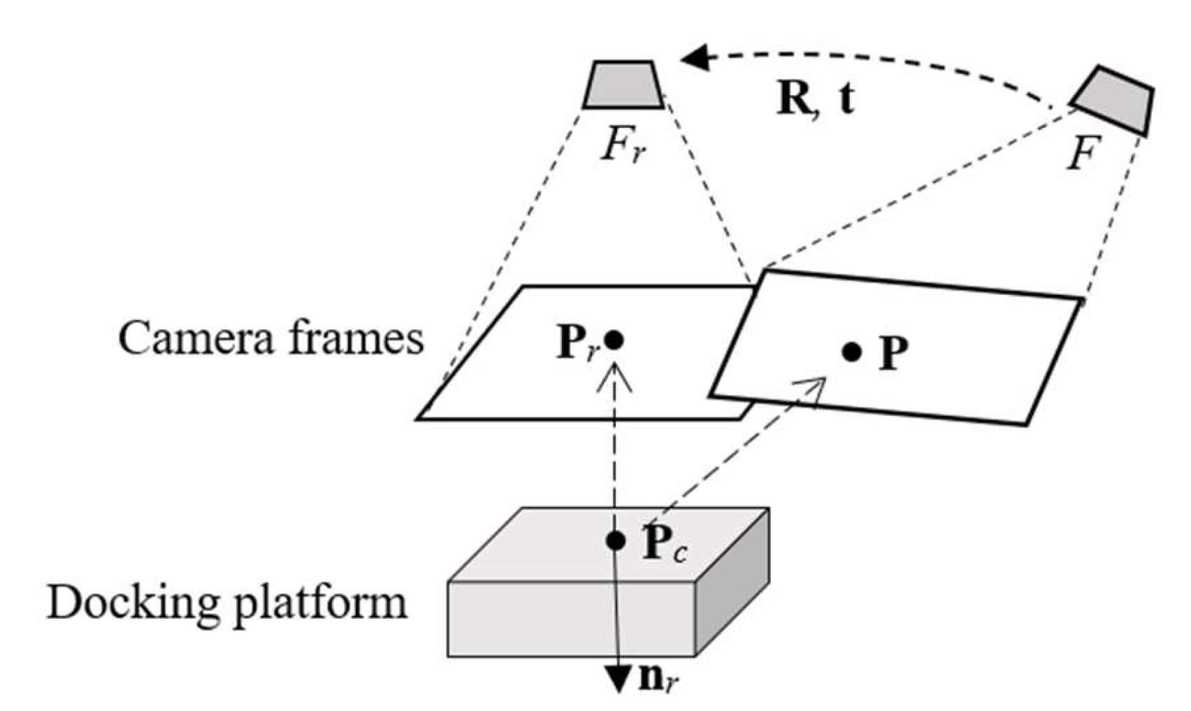
3.2. Visual Servo Docking Step

The target of the planar type docking is to land the AUV on the center of the docking platform. Let P_r = (X_r, Y_r, Z_r) = (0, 0, Z_r) be the platform center coordinate on the reference camera frame F_r when the AUV is right above the platform at (0, 0, 0). The AUV keeps its heading direction in parallel with the ocean current, which gives q ≈ 0, r ≈ 0, v_w ≈ 0. Equation (10) can then be simplified as:

$${\dot{e}}_v=\left[\begin{array}{c}{\dot{e}}_u\\ \begin{array}{l}{\dot{e}}_v\\ {\dot{e}}_w\end{array}\end{array}\right]=\left[\begin{array}{l}{u}_r+u_w\hfill \\ v_r-(-e_w+Z_r)p\hfill \\ w-e_{v}p\hfill \end{array}\right].$$

(30)

Recall the definition in (4), the aim of the docking step is to let (e_u, e_v, e_w) converge to (0, 0, Z_r). Hence, choosing the control law in the kinematic level as:

$$\begin{array}{l}{u}_r=-k_{eu}{e}_u-u_w,\hfill \\ p=\frac{v_r}{-e_w+Z_r}+k_{ev}{e}_v, \left(e_w<Z_r\right),\hfill \\ w=e_{v}p-k_{ew}(e_w-Z_r)+\left|w_0\right|,\hfill \end{array}$$

(31)

where the controller gains k_eu, k_ev, and k_ew are positive and $\left|w_0\right|$ provides a non-negative terminal velocity when the AUV touches the platform surface. Considering the Lyapunov function:

$$V_e\left(e_u,e_v,e_w\right)=\frac{1}{2}{e}_u^2+\frac{1}{2}{e}_v^2+\frac{1}{2}{\left(e_w-Z_r\right)}^2.$$

(32)

Bringing (31) into (30) with $w_0=0$, the time derivative of V_e is:

$$\begin{array}{l}{\dot{V}}_e=e_u\left(u_r+u_w\right)+e_v\left(v_r-(-e_w+Z_r)p\right)+\left(e_w-Z_r\right)\left(w-e_{v}p\right)\\ \hspace{1em} =-k_{eu}{e}_u^2-k_{ev}{e}_v^2-k_{ew}{\left(e_w-Z_r\right)}^2<0.\end{array}$$

(33)

The following lemma then establishes.

Lemma 3.

Considering the visual servo model in (9). Applying the controller in (31) and using the results of (33), the visual objective functions (e_u, e_v, e_w) are bounded and exponentially converge to (0, 0, Z_r) as $t\to \infty$.

Following the similar design procedure as above, the kinematic controller of the visual servo docking step is extended to the dynamic case. Let α_u2, α_p and α_w be the virtual control law, introducing the control errors:

$$\begin{array}{l}{z}_{u2}=u_r-{\alpha }_{u2},\\ z_p=p-{\alpha }_p,\\ z_w=w-{\alpha }_w,\end{array}$$

(34)

and the parameters to be estimated:

$${\theta }_v={\left(m_u, d_u, m_p, m_{vw}, d_p, m_w, m_v,d_w\right)}^{\mathrm{T}}.$$

(35)

Choosing the Lyapunov function:

$$V_{a2}(e_u,e_v,z_{u2},z_p,z_w,\tilde{\theta })=V_e+\frac{1}{2}{m}_u{z}_{u2}{}^2+\frac{1}{2}{m}_p{z}_p{}^2+\frac{1}{2}{m}_w{z}_w{}^2+\frac{1}{2}{\tilde{\theta }}_v{}^{\mathrm{T}}{\mathsf{\Gamma }}_v{}^{-1}{\tilde{\theta }}_v ,$$

(36)

the time derivative of V_a2 is:

$$\begin{array}{ll}{\dot{V}}_{a2}=& {\dot{V}}_e+m_u{z}_{u2}{\dot{z}}_{u2}+m_p{z}_p{\dot{z}}_p+m_w{z}_w{\dot{z}}_w-{\tilde{\theta }}_v{}^{\mathrm{T}}{\mathsf{\Gamma }}_v{}^{-1}{\dot{\widehat{\theta }}}_v\\ & =-k_{eu}{e}_u^2-k_{ev}{e}_v^2-k_{ew}{\left(e_w-Z_r\right)}^2+z_{u2}\left[{\tau }_{u2}-m_u{\dot{\alpha }}_{u2}-d_u{u}_r+e_u\right]\\ & +z_p\left[{\tau }_p-m_p{\dot{\alpha }}_p+m_{vw}{v}_{r}w-d_{p}p+m{z}_{g}pw-m{z}_{g}g\sin \varphi -2e_v(-e_w+Z_r)\right]\\ & +z_w\left[{\tau }_w-m_w{\dot{\alpha }}_w+m_v{v}_{r}p+m{z}_g{p}^2-d_{w}w+(e_w-Z_r)\right]-{\tilde{\theta }}_v{}^{\mathrm{T}}{\mathsf{\Gamma }}_v{}^{-1}{\dot{\widehat{\theta }}}_v.\end{array}$$

(37)

Choosing the control law in the dynamic level as:

$$\begin{array}{l}{\tau }_u={\widehat{m}}_u{\dot{\alpha }}_{u2}+{\widehat{d}}_u{u}_r-e_u-k_{\tau u2}{z}_{u2},\\ {\tau }_p={\widehat{m}}_p{\dot{\alpha }}_p-{\widehat{m}}_{vw}{v}_{r}w+{\widehat{d}}_{p}p+2e_v(-e_w+Z_r)-m{z}_{g}pw+m{z}_{g}g\sin \varphi -k_{\tau p}{z}_p,\\ {\tau }_w={\widehat{m}}_w{\dot{\alpha }}_w-{\widehat{m}}_v{v}_{r}p+{\widehat{d}}_{w}w-m{z}_g{p}^2-(e_w-Z_r)-k_{\tau w}{z}_w,\end{array}$$

(38)

and the adaptive law as:

$${\dot{\widehat{\theta }}}_v={\mathsf{\Gamma }}_v{\Phi }_v,$$

(39)

where

$${\Phi }_v={\left(-z_{u2}{\dot{\alpha }}_{u2},-z_u{u}_r,-z_p{\dot{\alpha }}_p, z_p{v}_{r}w,-z_{p}p, -z_w{\dot{\alpha }}_w, z_w{v}_{r}p,-z_{w}w\right)}^{\mathrm{T}}.$$

(40)

Applying (33), (38)–(40) into (37) yields:

$${\dot{V}}_{a2}=-k_{eu}{e}_u^2-k_{ev}{e}_v^2-k_{ew}{\left(e_w-Z_r\right)}^2-k_{\tau u2}{z}_{u2}{}^2-k_{\tau p}{z}_p{}^2-k_{\tau w}{z}_w{}^2<0,$$

(41)

which indicates that $\left(e_u,e_v,z_{u2},z_p,z_w\right)$ converges to zero and e_w converges to Z_r as $t\to \infty$.

It can then be concluded from (41) and Lemma 3 that for the visual servo docking process described by the kinematics in (10) and the dynamics in (13), applying the control laws in (31) and (38), the translation visual error e_v = (e_u, e_v, e_w) asymptotically converges to (0, 0, Z_r) as $t\to \infty$. Consequently, the distance from the platform center to the AUV camera center converges to zero as $t\to \infty$.

4. Simulation and Analysis

The physical parameters of the HOME-I AUV introduced in our previous work [15] are applied in the simulation in this paper, as shown in

Table 1. AUV dynamic parameters in the simulation.

$M_{RB}=\left[\begin{array}{cc}{M}_{RB}^{11}& M_{RB}^{12}\\ M_{RB}^{21}& M_{RB}^{22}\end{array}\right]$	$M_A=\left[\begin{array}{cc}{M}_A^{11}& M_A^{12}\\ M_A^{21}& M_A^{22}\end{array}\right]$	D = diag (Dv, Dω)
${\mathrm{M}}_{\mathrm{RB}}^{11}$ = diag(15, 15, 15) (kg)	$M_A^{11}=\left[\begin{array}{ccc}6& 0.1& 0\\ 0.1& 18& 0\\ 0& 0& 14\end{array}\right]$ (kg·m)	Dv = diag(8, 20, 30) (kg·s−1)
${\mathrm{M}}_{\mathrm{RB}}^{22}$ = diag(0.7, 0.55, 0.5) (kg·m2)	$M_A^{22}=\left[\begin{array}{ccc}0.2& 0& 0.01\\ 0& 0.5& 0\\ 0.01& 0& 0.5\end{array}\right]$ (kg·m2)	Dω = diag(1.5, 2.8, 3) (kg·m2·s−1)
$M_{RB}^{12}={\left(M_{RB}^{21}\right)}^{\mathrm{T}}=\left[\begin{array}{ccc}0& 0.6& 0\\ -0.6& 0& 0\\ 0& 0& 0\end{array}\right]$ (kg·m)	$M_A^{12}={\left(M_A^{21}\right)}^{\mathrm{T}}=\left[\begin{array}{ccc}0& 0.05& 0\\ 0.05& 0& 0.01\\ 0& 0.01& 0\end{array}\right]$ (kg·m)

. Notice that these parameters are regarded as true values of the AUV model, but are not utilized in the controllers. Instead, different estimated parameters are applied in the controller of each docking step.

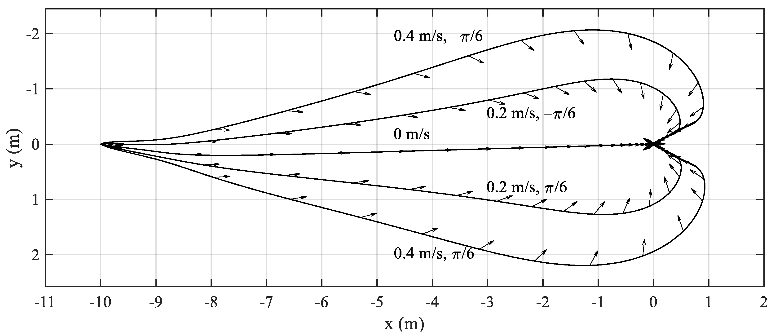
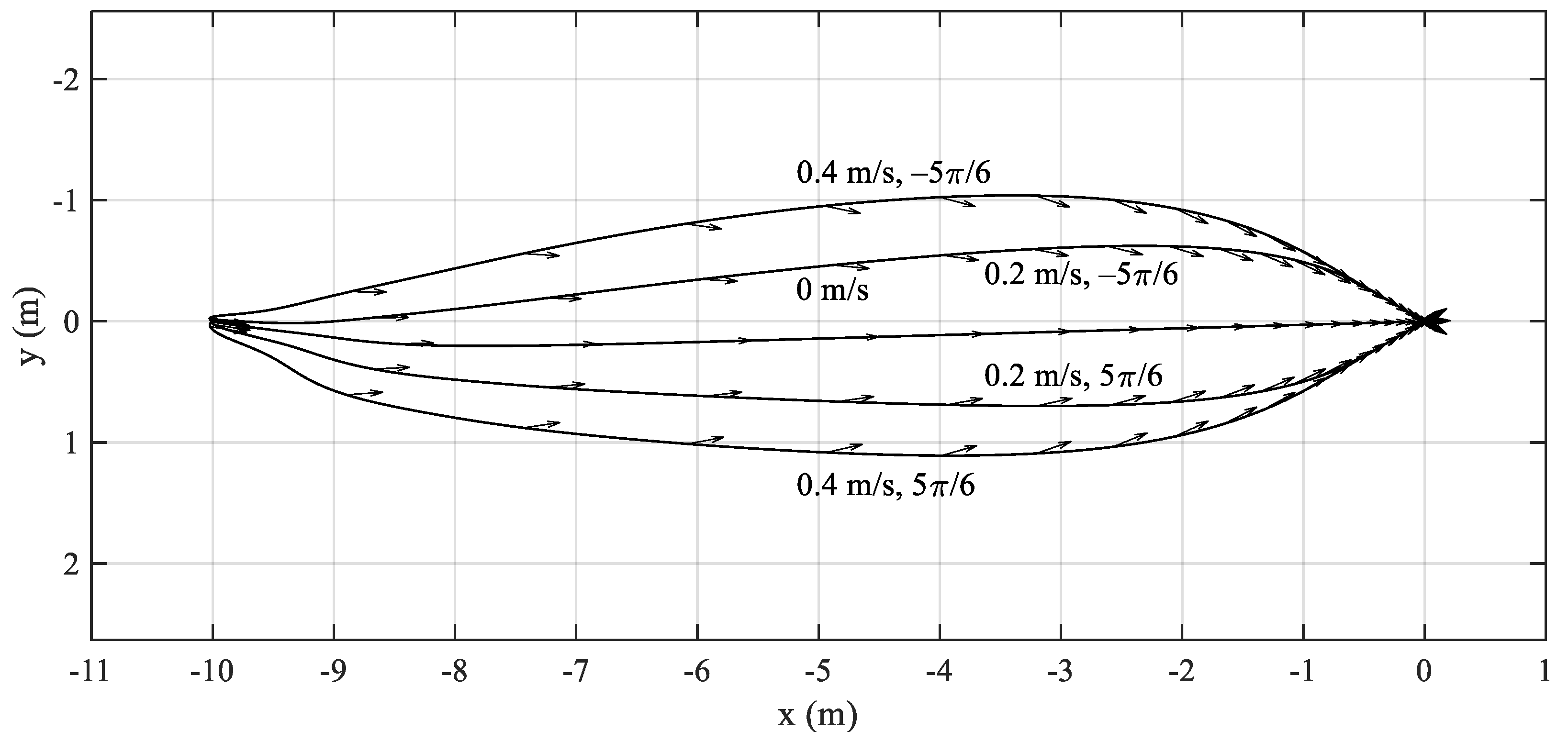
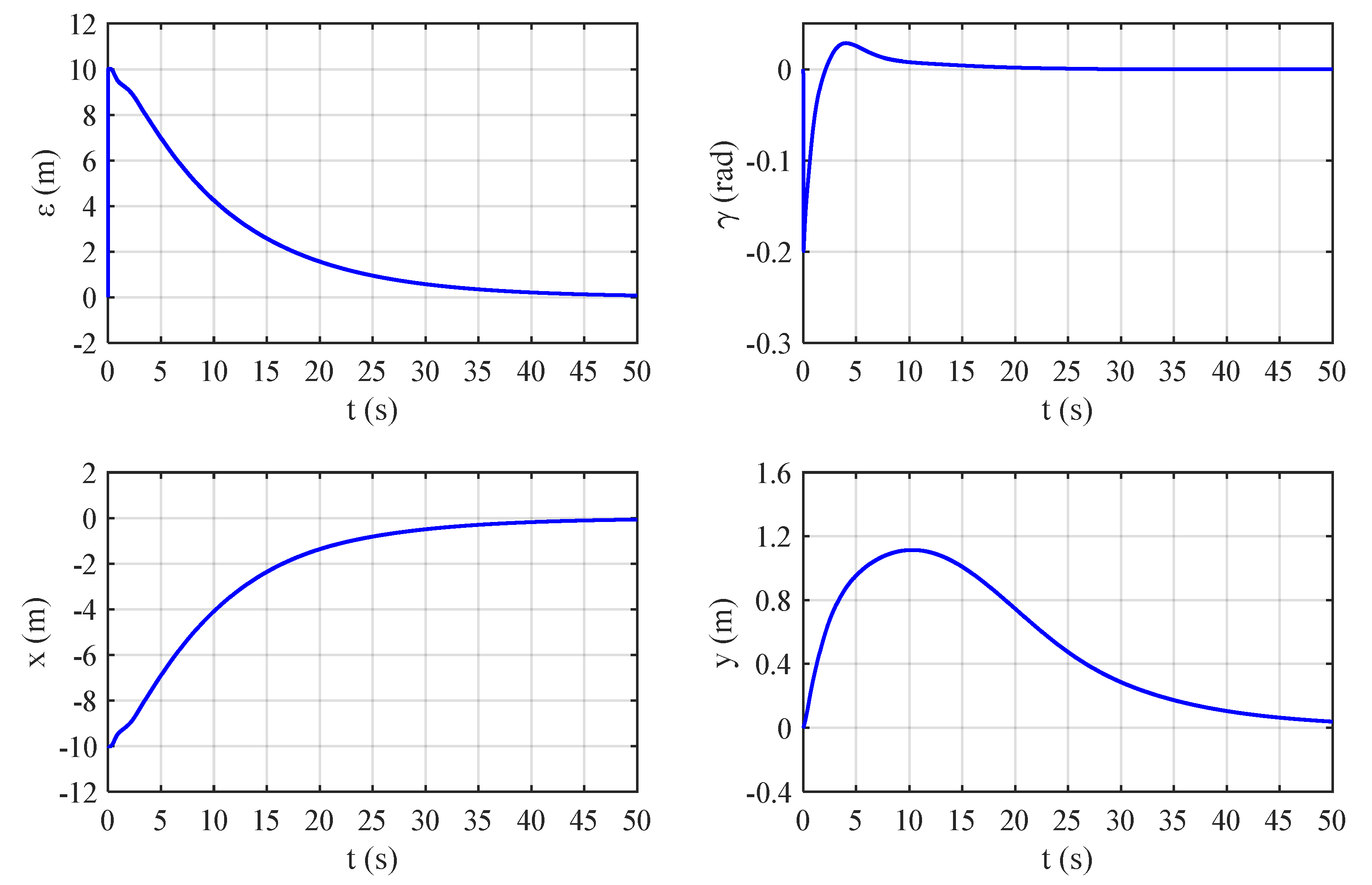
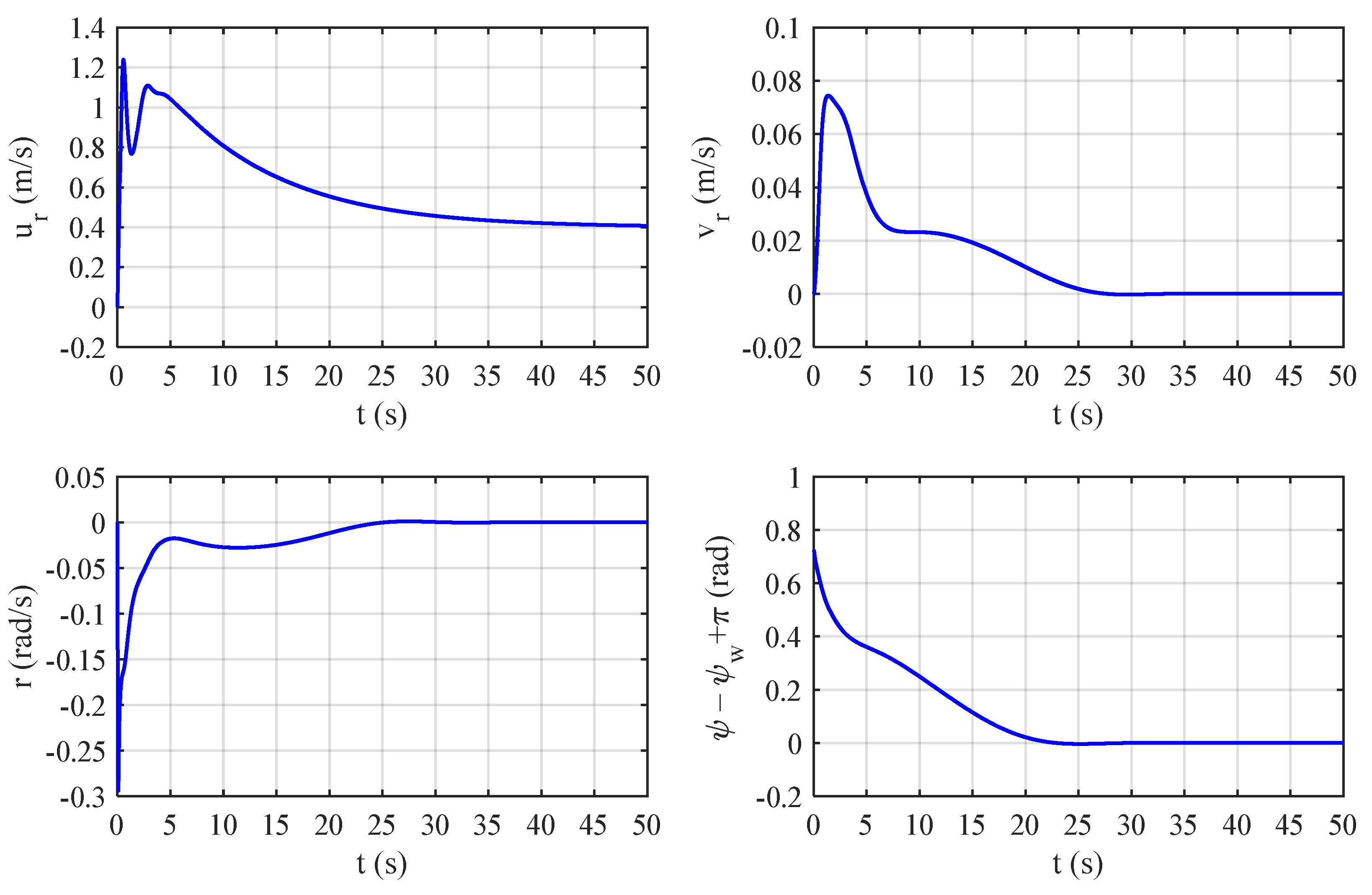
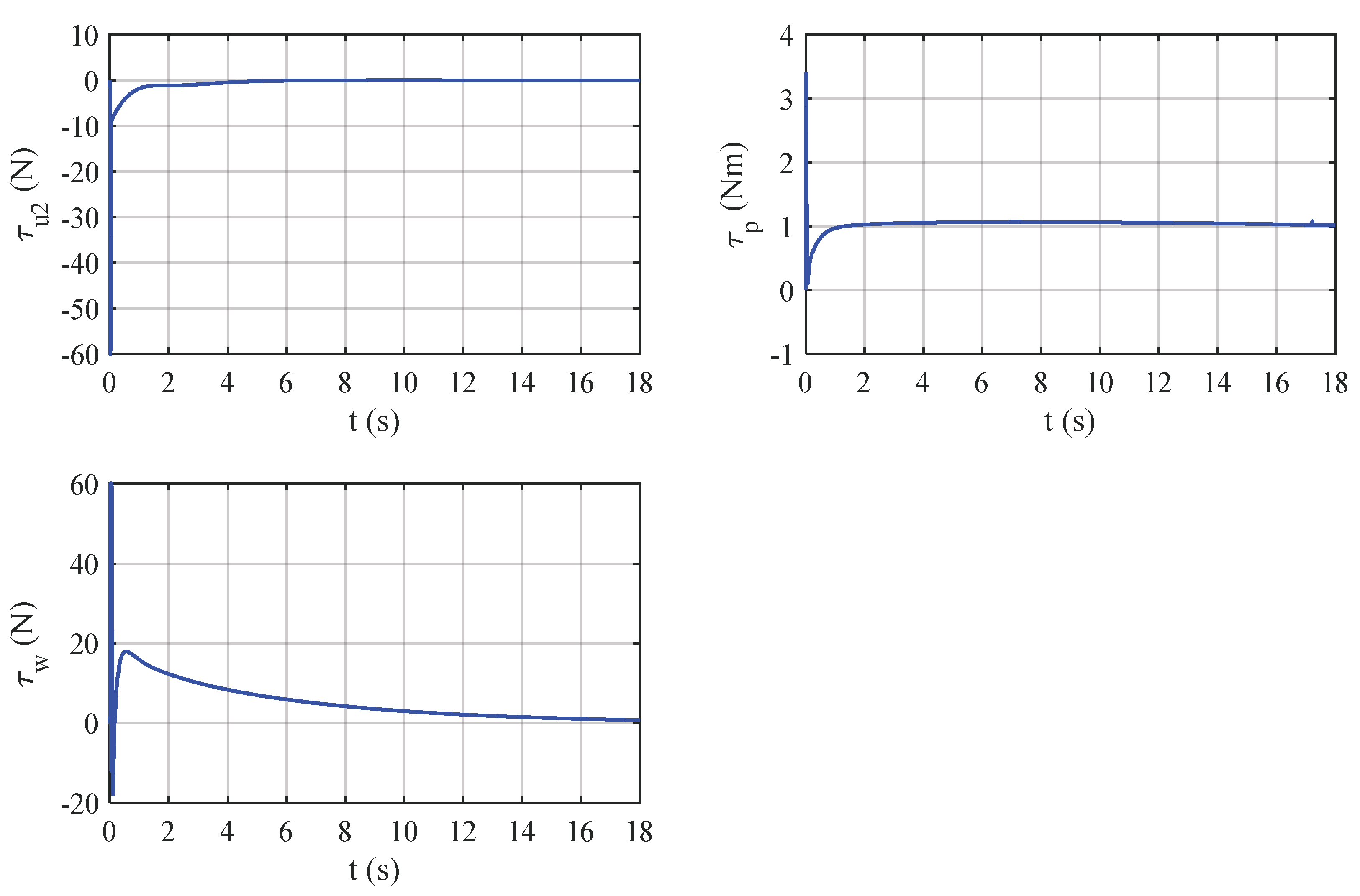
4.1. Pre-Docking Process

In order to validate the performance of the parameter adaption law, rough initial estimations with large estimation errors are adopted, where $\hat{\mathbf{\theta }}$ = (15, 20, 10, 0.1, 1, 1)^T. The parameter adaption law is chosen to be $\mathsf{\Gamma }$ = 100 × diag(2, 5, 2, 1, 1, 1). The starting point is chosen as (x₀, y₀, ψ₀) = (−10, 0, 0.2), and the target point is (x_d, y_d) = (0, 0). The observer gains are chosen as k_ox1 = k_oy1 = 2, k_ox2 = k_oy2 = 1. The initial current estimation is v_wx0 = v_wy0 = 0.2. The controller gains are chosen as k_u = 0.1, k_r = 1, k_τu = 50, k_τr = 20. The ocean current disturbances with different velocities and directions are set to evaluate the controlling performance. The simulation trajectories are plotted in Figure 5 and Figure 6.

The arrows in Figure 5 and Figure 6 denote the heading direction of the AUV. The trajectory under current disturbance is the current dependent curves instead of straight lines. The AUV goes upstream against the current when the ocean current has an angle of ψ_w = ±5π/6, while runs downstream when the current angle is ψ_w = ±π/6. The trajectories are generally shorter when sailing upstream, and the trajectory deviations under 0.4 m/s current disturbance are approximately twice as large as those under 0.2 m/s current with the same direction. The AUV slows down when approaching the destination point, so that the arrows become more intensive as the distance error $\epsilon$ becomes smaller. The yaw angle of the AUV finally converges to an antiparallel direction with the current, so that the current influence on the sway motion can be minimized during the visual servo docking step.

An ocean current of V_w = 0.4 m/s and ψ_w = 5π/6 is taken as an example to investigate the changes of the state variables during the pre-docking process. The results are shown in Figure 7 and Figure 8.

In Figure 7, $\epsilon$, γ, x and y all converge within t = 50 s. The direction error γ converges within t = 20 s, which is much faster than the position error $\epsilon$ and guarantees a stable control performance. The maximum lateral deviation of 1.2 m occurs at about t = 10 s and then gradually decreases as the direction error γ converges.

In Figure 8, the yaw velocity r stays below 0.05 rad/s after t = 5 s and the surge velocity u_r does not exceed 1.3 m/s, which are all capable and realistic for the prototype miniaturized AUV. The underactuated sway velocity v_r is an order of magnitude smaller than u_r, which indicates a stable motion control. The convergence of ψ − ψ_w to −π indicates an antiparallel dynamic positioning direction of the AUV in the destination point.

The thrusting force and torque are plotted in Figure 9. The upper bounds of τ_u and τ_r are set to be 60 N and 10 Nm respectively to match up with the physical limitations of the AUV thrusters. However, the upper bounds are only at the starting point, and τ_u and τ_r change smoothly within the time interval. The force τ_u stays below 20 N and the torque stays far below 1 Nm during the whole process, which are all capable of the real system. Therefore, the controller is practical and energy efficient in real applications.

4.2. Visual Servo Docking Process

The visual servo docking step is simulated under the premise that the pre-docking step is successfully finished. The ocean current is canceled and thus is excluded in the visual servo docking process. A vessel parallel (VP) coordinate is introduced with a coordinate transformation of η_p = R^T(ψ)η to transform the visual servo objective function to the NED frame position. The origin O_p is fixed on the dynamic positioning plane right above the platform center.

Although the AUV is expected to stay right above the docking platform center after the pre-docking process, a positioning error is inevitable in reality. Therefore, an initial positioning error is considered in the docking process. Choosing the platform center in the VP coordinate at P_c = (0, 0, 3) and setting an initial positioning error of x_p = y_p = 0.5. An initial parameter estimation with large estimation error is adopted as ${\hat{\mathsf{\theta }}}_v$ = (15, 10, 0.2, 0, 0.5, 15, 20, 15)^T, the adaption gain is chosen as ${\mathsf{\Gamma }}_v$ = 100 × diag(1, 1, 0.1, 0.1, 0.1, 0.5, 1, 1). The controller parameters are k_eu = 0.7, k_ev = 0.5, k_ew = 0.17, k_τu2 = 30, k_τw = 40, k_τp = 10 and w₀ = 0.03. The results are plotted in Figure 10, Figure 11 and Figure 12.

It can be observed from Figure 10 that the objective function e_u and e_v exponentially converge to zero and the e_w converges to Z_r. The initial value of x_p and y_p come from the positioning error of the pre-docking process and are gradually eliminated during the landing process. The maximum tolerance of the initial dynamic positioning error is positively related to the vertical landing distance. According to the coordinate transformation relationships, e_u and x_p are coincident, e_w and z_p are almost coincident. However, e_v rapidly converges in less than 3 s by the roll angle adjustment, which is much faster than y_p, because the real lateral position error must be gradually eliminated during the docking process. The roll motion is kept within 0.2 rad during the landing process, which has little influence on the motion stability. The roll angle should be limited to guarantee a stable pose of the AUV and a successful recognition of the docking platform pattern.

Figure 11 shows the velocity components during the docking process. All the translational and angular velocities are smoothly and gently adjusted except at the starting point. The absolute value of the surge velocity u_r does not exceed 0.2 m/s during the whole process. The sway velocity brought by the roll motion adjustment is much smaller than the surge velocity and quickly converges in 10 s. Due to the small damping along the x axis, the roll motion adjustment almost completes within 4 s and the roll velocity p is almost zero during the rest of the docking process. The heave velocity w reaches up to 0.4 m/s and smoothly decreases during the rest of the time.

Figure 12 shows the corresponding driving forces and torque. The forces τ_u2, τ_p and torque τ_w are all within practical ranges and change smoothly during the process except at the starting point. The force τ_u2 is very small all the time, and the torque τ_p is kept at about 1 Nm to keep a roll angle for the AUV. The force τ_w is transitorily large and reaches the upper bound of 60 N within 1 s, and kept below 20 N during the rest of the time. The results demonstrate that the visual servo docking controller is practical and energy efficient for the real prototype AUV.

In general, the two steps of the proposed controller are stable, concise and well cooperated. The controller successfully deals with the ocean current disturbance and the model parameter uncertainties, and provides a stable and accurate planar type docking control.

5. Conclusions

A two-step adaptive controller for planar type docking is investigated in this paper. It makes a seamless combination of horizontal dynamic positioning and vertical visual servo to achieve a stable and accurate control performance. The control method not only takes full advantage of the omnidirectional feature of the planar type docking station, but also perfectly matches up with the underactuated feature of the prototype AUV. Practical issues are fully considered in the design process and simulation validation, including model parameter uncertainties, unknown ocean current disturbances, hardware limitations and inevitable positioning errors.

Future work will investigate more essential issues involved in the practical application of the method. Practical issues include measurement noise, water turbidity and targe occlusion need to be considered in the complex ocean environment. Applying the algorithm to different types of AUVs with various propulsion and sensor configurations is also regarded as an extension of the proposed work. The authors believe that this work provides valuable reference for related fields.

References

1. Wu, Y.; Ta, X.; Xiao, R.; Wei, Y.; An, D.; Li, D. Survey of underwater robot positioning navigation. Appl. Ocean Res. 2019, 90, 101845. [Google Scholar] [CrossRef]
2. Sahoo, A.; Dwivedy, S.K.; Robi, P. Advancements in the field of autonomous underwater vehicle. Ocean Eng. 2019, 181, 145–160. [Google Scholar] [CrossRef]
3. Nayak, N.; Das, S.R.; Panigrahi, T.K.; Das, H.; Nayak, S.R.; Singh, K.K.; Askar, S.S.; Abouhawwash, M. Overshoot Reduction Using Adaptive Neuro-Fuzzy Inference System for an Autonomous Underwater Vehicle. Mathematics 2023, 11, 1868. [Google Scholar] [CrossRef]
4. Yazdani, A.; Sammut, K.; Yakimenko, O.; Lammas, A. A survey of underwater docking guidance systems. Robot. Auton. Syst. 2020, 124, 103382. [Google Scholar] [CrossRef]
5. Stokey, R.; Purcell, M.; Forrester, N.; Austin, T.; Goldsborough, R.; Allen, B.; von Alt, C. A Docking System for REMUS, an Autonomous Underwater Vehicle. In Proceedings of the IEEE/MTS OCEANS 1997 Conference, Halifax, NS, Canada, 6–9 October 1997; pp. 1132–1136. [Google Scholar]
6. Teeneti, C.R.; Truscott, T.T.; Beal, D.N.; Pantic, Z. Review of Wireless Charging Systems for Autonomous Underwater Vehicles. IEEE J. Ocean. Eng. 2019, 46, 68–87. [Google Scholar] [CrossRef]
7. Li, H.; Huang, F.; Chen, Z. Virtual-reality-based online simulator design with a virtual simulation system for the docking of unmanned underwater vehicle. Ocean Eng. 2022, 266, 112780. [Google Scholar] [CrossRef]
8. Lin, M.; Lin, R.; Yang, C.; Li, D.; Zhang, Z.; Zhao, Y.; Ding, W. Docking to an underwater suspended charging station: Systematic design and experimental tests. Ocean Eng. 2022, 249, 110766. [Google Scholar] [CrossRef]
9. Palomeras, N.; Vallicrosa, G.; Mallios, A.; Bosch, J.; Vidal, E.; Hurtos, N.; Carreras, M.; Ridao, P. AUV homing and docking for remote operations. Ocean Eng. 2018, 154, 106–120. [Google Scholar] [CrossRef]
10. Palomer, A.; Ridao, P.; Ribas, D. Inspection of an underwater structure using point-cloud SLAM with an AUV and a laser scanner. J. Field Robot. 2019, 36, 1333–1344. [Google Scholar] [CrossRef]
11. Allibert, G.; Hua, M.-D.; Krupínski, S.; Hamel, T. Pipeline following by visual servoing for Autonomous Underwater Vehicles. Control Eng. Pract. 2019, 82, 151–160. [Google Scholar] [CrossRef] [Green Version]
12. Nguyen, L.-H.; Hua, M.-D.; Allibert, G.; Hamel, T. A Homography-Based Dynamic Control Approach Applied to Station Keeping of Autonomous Underwater Vehicles Without Linear Velocity Measurements. IEEE Trans. Control Syst. Technol. 2020, 29, 2065–2078. [Google Scholar] [CrossRef]
13. Kimball, P.W.; Clark, E.B.; Scully, M.; Richmond, K.; Flesher, C.; Lindzey, L.E.; Harman, J.; Huffstutler, K.; Lawrence, J.; Lelievre, S.; et al. The Artemis under-ice AUV docking system. J. Field Robot. 2018, 35, 299–308. [Google Scholar] [CrossRef]
14. Myint, M.; Yonemori, K.; Lwin, K.N.; Yanou, A.; Minami, M. Dual-eyes Vision-based Docking System for Autonomous Underwater Vehicle: An Approach and Experiments. J. Intell. Robot. Syst. 2018, 92, 159–186. [Google Scholar] [CrossRef]
15. Wang, T.; Zhao, Q.; Yang, C. Visual navigation and docking for a planar type AUV docking and charging system. Ocean Eng. 2021, 224, 108744. [Google Scholar] [CrossRef]
16. Akinyele, O.; Choi, J.W.; Yu, C.H. Improving Response Performance of Quadrant-detector-navigated Unmanned Underwater Vehicle in Underwater Docking Operations. Int. J. Control Autom. Syst. 2021, 19, 1013–1025. [Google Scholar] [CrossRef]
17. Zhang, Y.; Gao, J.; Chen, Y.; Bian, C.; Zhang, F.; Liang, Q. Adaptive neural network control for visual docking of an autonomous underwater vehicle using command filtered backstepping. Int. J. Robust Nonlinear Control 2022, 32, 4716–4738. [Google Scholar] [CrossRef]
18. Xie, T.; Li, Y.; Jiang, Y.; Pang, S.; Wu, H. Turning circle based trajectory planning method of an underactuated AUV for the mobile docking mission. Ocean Eng. 2021, 236, 109546. [Google Scholar] [CrossRef]
19. Ren, R.; Zhang, L.; Liu, L.; Yuan, Y. Two AUVs Guidance Method for Self-Reconfiguration Mission Based on Monocular Vision. IEEE Sens. J. 2021, 21, 10082–10090. [Google Scholar] [CrossRef]
20. Yan, Z.; Zhang, J.; Tang, J. Whale optimization algorithm based on lateral inhibition for image matching and vision-guided AUV docking. J. Intell. Fuzzy Syst. 2021, 40, 4027–4038. [Google Scholar] [CrossRef]
21. Aguiar, A.P.; Pascoal, A.M. Dynamic positioning and way-point tracking of underactuated AUVs in the presence of ocean currents. Int. J. Control 2007, 80, 1092–1108. [Google Scholar] [CrossRef]
22. Panagou, D.; Kyriakopoulos, K.J. Dynamic positioning for an underactuated marine vehicle using hybrid control. Int. J. Control 2014, 87, 264–280. [Google Scholar] [CrossRef]
23. Wang, Y.-L.; Han, Q.-L.; Fei, M.-R.; Peng, C. Network-Based T–S Fuzzy Dynamic Positioning Controller Design for Unmanned Marine Vehicles. IEEE Trans. Cybern. 2018, 48, 2750–2763. [Google Scholar] [CrossRef] [PubMed] [Green Version]
24. Gao, J.; Liu, C.; Proctor, A. Nonlinear model predictive dynamic positioning control of an underwater vehicle with an onboard USBL system. J. Mar. Sci. Technol. 2016, 21, 57–69. [Google Scholar] [CrossRef]
25. Elmokadem, T.; Zribi, M.; Youcef-Toumi, K. Control for Dynamic Positioning and Way-point Tracking of Underactuated Autonomous Underwater Vehicles Using Sliding Mode Control. J. Intell. Robot. Syst. 2019, 95, 1113–1132. [Google Scholar] [CrossRef]
26. Peng, Y.; Guo, L.; Meng, Q.; Chen, H. Research on Hover Control of AUV Uncertain Stochastic Nonlinear System Based on Constructive Backstepping Control Strategy. IEEE Access 2022, 10, 50914–50924. [Google Scholar] [CrossRef]
27. Benhimane, S.; Malis, E. Homography-based 2D Visual Tracking and Servoing. Int. J. Robot. Res. 2007, 26, 661–676. [Google Scholar] [CrossRef]
28. van der Zwaan, S.; Bernardino, A.; Santos-Victor, J. Visual station keeping for floating robots in unstructured environments. Robot. Auton. Syst. 2002, 39, 145–155. [Google Scholar] [CrossRef] [Green Version]
29. Krupinski, S.; Allibert, G.; Hua, M.-D.; Hamel, T. An Inertial-Aided Homography-Based Visual Servo Control Approach for (Almost) Fully Actuated Autonomous Underwater Vehicles. IEEE Trans. Robot. 2017, 33, 1041–1060. [Google Scholar] [CrossRef] [Green Version]
30. Gao, J.; Zhang, G.; Wu, P.; Zhao, X.; Wang, T.; Yan, W. Model Predictive Visual Servoing of Fully-Actuated Underwater Vehicles With a Sliding Mode Disturbance Observer. IEEE Access 2019, 7, 25516–25526. [Google Scholar] [CrossRef]
31. Wang, N.; He, H. Extreme Learning-Based Monocular Visual Servo of an Unmanned Surface Vessel. IEEE Trans. Ind. Informatics 2020, 17, 5152–5163. [Google Scholar] [CrossRef]
32. Gao, J.; Proctor, A.A.; Shi, Y.; Bradley, C. Hierarchical Model Predictive Image-Based Visual Servoing of Underwater Vehicles With Adaptive Neural Network Dynamic Control. IEEE Trans. Cybern. 2015, 46, 2323–2334. [Google Scholar] [CrossRef] [PubMed]
33. Fossen, T.I. Handbook of Marine Craft Hydrodynamics and Motion Control; Wiley: New York, NY, USA, 2011. [Google Scholar]
Figure 1. Planar type docking concept of a HOME-I AUV and docking station.
Mathematics 11 03467 g001
Figure 2. Reference frames and models of the AUV. (a) Reference frames. (b) Coordinate transformation.
Mathematics 11 03467 g002
Figure 3. Visual servo docking schematic.
Mathematics 11 03467 g003
Figure 4. Control diagram of the two-step adaptive docking controller.
Mathematics 11 03467 g004
Figure 5. Pre-docking step trajectories with different ocean currents of ψw = ±π/6.
Mathematics 11 03467 g005
Figure 6. Pre-docking step trajectories with different ocean currents of ψw = ±5π/6.
Mathematics 11 03467 g006
Figure 7. Position related variables versus time when Vw = 0.4 m/s and ψw = 5π/6.
Mathematics 11 03467 g007
Figure 8. Velocity related variables versus time when Vw = 0.4 m/s and ψw = 5π/6.
Mathematics 11 03467 g008
Figure 9. Force τu and torque τr versus time when Vw = 0.4 m/s and ψw = 5π/6.
Mathematics 11 03467 g009
Figure 10. Visual errors, position errors and roll angle during the docking process.
Mathematics 11 03467 g010
Figure 11. Translational and angular velocities during the docking process.
Mathematics 11 03467 g011
Figure 12. Forces and torque during the docking process.
Mathematics 11 03467 g012