Outer Synchronization of Two Muti-Layer Dynamical Complex Networks with Intermittent Pinning Control

Abstract

This paper regards the outer synchronization of multi-layer dynamical networks with additive couplings via aperiodically intermittent pinning control, in which different layers of each multi-layer network have different topological structures. First, a state-feedback intermittent pinning controller is designed in the drive and response configuration, and sufficient conditions to achieve the outer synchronization are derived based on the Lyapunov stability theory and matrix inequalities. Second, outer synchronization problem of multi-layer networks is discussed by setting an adaptive intermittent pinning controller; an appropriate Lyapunov function is selected to prove the criteria of synchronization between the drive multi-layer network and the response multi-layer network. Finally, three simulation examples are given to show the effectiveness of our control schemes.

1. Introduction

In the real world, there are various types of complex networks, such as the Internet, WWW (World Wide Web), transportation networks, neural networks, social networks, and so on. In the past 20 years, complex networks have been extensively studied regarding structural characteristics and dynamic behavior. Then, synchronization can describe the collective dynamics of the states of each node in complex networks, and has received high attention due to its many potential applications in automatic control [1,2], biological systems [1,3], secure communication [4], etc. In the last two decades, many important advances have been made in the research of the synchronization of complex networks; see the review literature [1,5,6]. However, previous research of the synchronization of complex networks mainly focused on single-layer networks (traditional complex networks). In the real environment, some complex networks have more than one layer, whose structures are more complicated. For example, in transportation networks, there may be roads, railways, and aviation among cities. In order to simulate such complex systems more accurately, the concept of multi-layer complex networks was proposed, and multi-layer complex networks have become a new research direction for the development of complex networks. Multi-layer complex networks take different kinds of interactions for multiple sub-networks into considerations. The synchronization of multi-layer networks has different types, and is usually divided into intra-layer synchronization [7,8,9,10], inter-layer synchronization [7,8], complete synchronization [7,8,11], etc. In addition, there is also outer synchronization, which refers to synchronization between different complex networks. The outer synchronization researches in complex networks can be found in the literature [12,13,14]. For the outer synchronization of the single-layer networks, Wang et al. [12] studied the synchronization between two delay-coupled complex dynamical networks with a noise perturbation using an adaptive controller. Hymavathi et al. [13] introduced an outer synchronization scheme for fractional-order neural networks with time delays, and derived several criteria achieving synchronization between the drive and response systems based on fractional inequalities and Lyapunov-type functions. Zhuang et al. [14] used drive-response methods to study the synchronization of multi-layer dynamical networks with additive delay couplings and stochastic perturbations, and obtained sufficient conditions for synchronization between the drive and response networks using pinning controllers. In the existing work of outer synchronization in complex networks, one usually designs some suitable control protocols to drive the synchronization of networks. To reduce control costs, some feasible control methods have been proposed, such as intermittent control [15,16,17,18,19,20,21,22], impulsive control [23,24], event-triggered control [25,26,27], pinning control [14,28,29,30,31,32,33], and so on.

Intermittent control is a common discontinuous control method, which has the advantages of a low cost, easy implementation, and strong flexibility. As early as 2000, the intermittent control method was applied to control dynamical systems. Subsequently, the control method was introduced to the synchronization of complex networks, for instance, periodically intermittent control [16,17,18,19]. Aperiodically (non-periodically) intermittent control has a wider range of applications. In [20], a synchronization scheme of complex networks with time-varying delays was investigated via the aperiodically intermittent control method, and an exponential synchronization criterion is obtained when the control ratio of the control width to the total time width is equal in any time interval. Li et al. [21] proposed an aperiodically intermittent control method, with which they studied the cluster synchronization problem of two-layer networks with time-varying delays, and deduced some criteria for cluster synchronization using a theoretical analysis. In [22], based on the aperiodically intermittent control method, the synchronization of multi-layer neural networks with coupled time-varying delays was studied, and the sufficient conditions for achieving global asymptotic synchronization were proved by using generalized Halanay inequalities.

For some complex networks with a large number of nodes, it is of important significance to control a fractional of nodes in networks to achieve synchronization. Wang and Chen [28] first applied the pinning control method to study the synchronization of scale-free networks. The pinning control method is more practical, and its control cost is lower, so the method has been a common control technique in complex networks. By using the pinning method, many achievements have been obtained in the synchronization of the single-layer networks [28,29,30]. Additionally, the pinning control has been used to study the synchronization problem of multi-layer dynamical networks [14,31,33].

In the paper, we will use an aperiodically intermittent control method to study outer synchronization for two multi-layer dynamic networks with additive couplings. It is observed that the synchronization problem of multi-layer networks with additive couplings has been studied in [14,34,35]. Reference [34] discussed the synchronization of multi-layer multi-agent systems with an additive coupling and Markovian switching coupling, and derived a synchronization region under two cases for multiple Laplacian matrices of networks. In 2020, Zhuang et al. [35] reported the synchronization of stochastic delayed multi-layer networks with additive couplings, and gave several sufficient conditions to guarantee the synchronization of stochastic delayed coupled multi-layer networks. Motivated by the above, this paper will use pinning and intermittent control methods to discuss outer synchronization for two multi-layer dynamic networks with additive couplings, and also obtain sufficient conditions under linear feedback control and adaptive control, respectively. Finally, three simulation examples are given to show the effectiveness of linear feedback and adaptive control methods. Compared with previous work, the main differences and contributions can be summarized: (1) In [34,35], the synchronization of multi-layer networks with additive coupling is studied with the pinning feedback control. Differently, we adopt the aperiodically intermittent pinning control, which shows better economy; (2) without utilizing the pining control in [21,22] for the synchronization of a multi-layer dynamic network, we combine the pining control and aperiodically intermittent control, and the additive coupling is considered in our model. (3) Research on the outer synchronization of two multi-layer networks with additive couplings was studied in the previous literature [14]; we study the outer synchronization of multi-layer networks by using intermittent pinning control.

This paper is organized as follows. In Section 2, notations, models of multi-layer networks with additive couplings, a hypothesis, and some lemmas are introduced. In Section 3, the main content on outer synchronization is presented. In Section 4, numerical simulations are given to further verify the correctness of the main results. The conclusions are given in Section 5.

2. Model Description and Preliminaries

In the paper, the following notations are adopted. $\mathcal{N}$ is the set of natural numbers, $R^n$ denotes n-dimensional real column vectors, and $I^n$ denotes the identity matrix with order n. The superscript T represents the transpose operation to a corresponding matrix (or vector). For two symmetric matrices P and Q, P < 0 (P ≥ 0) means that the matrix P is a negative (non-negative) definite matrix and P ≤ Q (P ≥ Q) means that the matrix P − Q (P − Q) is a negative (positive) semi-definite matrix.

We consider an outer synchronization model for two multi-layer dynamic networks with additive couplings, and assume that node-to-node has achieved inter-layer synchronization in a multi-layer complex network. To achieve the synchronization of two multi-layer dynamic networks, add intermittent pinning controllers in the response systems. Without a loss of generality, let us assume that intermittent controllers only pin the first l nodes.

The drive-response multi-layer dynamical networks are as follows:

$${\dot{x}}_i(t)=f(x_i(t))+{\displaystyle \sum _{k=1}^M{c}_k{\displaystyle \sum _{j=1}^N{a}_{ij}^{(k)}D(x_j(t)-x_i(t))}}$$

(1)

$${\dot{y}}_i(t)=\left\{\begin{array}{l}f(y_i(t))+{\displaystyle \sum _{k=1}^M{c}_k{\displaystyle \sum _{j=1}^N{a}_{ij}^{(k)}D(y_j(t)-y_i(t))}}+u_i(t),i=1,2,\dots ,l\\ f(y_i(t))+{\displaystyle \sum _{k=1}^M{c}_k{\displaystyle \sum _{j=1}^N{a}_{ij}^{(k)}D(y_j(t)-y_i(t)),i=l+1,\dots ,N}}\end{array}\right.$$

(2)

where N ($\in \mathcal{N}$) is the number of nodes of each layer, $x_i(t)={[x_{i1}(t),x_{i2}(t),\dots ,x_{in}(t)]}^{{\rm T}}$ and $y_i(t)={[y_{i1}(t),y_{i2}(t),\dots ,y_{in}(t)]}^{{\rm T}}$$\in R^n$ are the state vectors of the ith node of drive-response multi-layer networks, $f(.):R^n\to R^n$ is a smooth nonlinear vector field, and $M\in \mathcal{N}$ is the number of layers. $c_k>0$ is the strength of coupling contributed with the kth layer, and $A^{(k)}={(a_{ij}^{(k)})}_{N\times N}$ is the outer coupling matrix (irreducible); if there is a coupling link from node i to node j (j ≠ i), then $a_{ij}^{(k)}>0$, otherwise, $a_{ij}^{(k)}=0$, which satisfies the diffusion property ${\displaystyle \sum _{j=1}^N{a}_{ij}^{(k)}}$$={\displaystyle \sum _{j=1}^N{a}_{ji}^{(k)}}=0$, $i=1,2,\dots ,N$, $k=1,2,\dots ,M$; $D=diag(d_1,d_2,\dots ,d_n)$ is an inner coupling matrix in each layer ($d_i>0,i=1,2,\dots ,n$), and $u_i(t)$ is a state-feedback controller with constant control gains or an adaptive controller in the ith node.

Aperiodically intermittent control divides the entire control time into a series of unequal time slots, the jth time slot is $T_j=[t_j,t_{j+1})$. Note that $[t_j,t_j+h_j)$ and $[t_j+h_j,t_{j+1})$ are the control time and non-control time regarding the jth time slot, respectively; then, $h_j$ is control width, and ${\overline{h}}_j=t_{j+1}-(t_j+h_j)$ is non-control width in the jth time slot, $j\in \mathcal{N}$.

With the properties of the diffusive matrix, Equations (1) and (2) can be rewritten as

$${\dot{x}}_i(t)=f(x_i(t))+{\displaystyle \sum _{k=1}^M{c}_k{\displaystyle \sum _{j=1}^N{a}_{ij}^{(k)}D{x}_j(t)}},i=1,2,\dots ,N$$

(3)

$${\dot{y}}_i(t)=\left\{\begin{array}{l}f(y_i(t))+{\displaystyle \sum _{k=1}^M{c}_k{\displaystyle \sum _{j=1}^N{a}_{ij}^{(k)}D{y}_j(t)}}+u_i(t),i=1,2,\dots l\\ f(y_i(t))+{\displaystyle \sum _{k=1}^M{c}_k{\displaystyle \sum _{j=1}^N{a}_{ij}^{(k)}D{y}_j(t),i=l+1,\dots ,N}}\end{array}\right.$$

(4)

Define the error vector as

$$e_i(t)=y_i(t)-x_i(t),i=1,2,\dots ,N$$

(5)

From Equations (3) and (4), one has the following error equations:

$${\dot{e}}_i(t)=\left\{\begin{array}{l}f(y_i(t))-f(x_i(t))+{\displaystyle \sum _{k=1}^M{c}_k{\displaystyle \sum _{j=1}^N{a}_{ij}^{(k)}De(t)}}+u_i(t),i=1,2,\dots ,l\\ f(y_i(t))-f(x_i(t))+{\displaystyle \sum _{k=1}^M{c}_k{\displaystyle \sum _{j=1}^N{a}_{ij}^{(k)}De(t)}},i=l+1,\dots ,N\end{array}\right.$$

(6)

Next, a definition of outer synchronization for two multi-layer complex networks, a hypothesis, and some lemmas are presented for later use.

Definition 1.

The multi-layer complex networks (1) and (2) achieve outer synchronization if$\underset{t\to \infty }{ \lim }{e}_i(t)=0$, for$i=1,2,\dots ,N$.

Hypothesis 1.

There exists a$\rho >0$, for$x,y\in R^n$and a matrix$\Omega \in R^{n\times n}$, such that$f(\cdot )$satisfies

$${(x-y)}^{{\rm T}}(f(x)-f(y)\le \rho {(x-y)}^{{\rm T}}\Omega (x-y)$$

where$\Omega =diag({\omega }_1,{\omega }_2,\dots ,{\omega }_n)$,${\omega }_i$is a positive constant, and $i=1,2,\dots ,n$.

Lemma 1 ([36]).

If$A_{m\times m}\ge 0,B_{m\times m}\ge 0,C_{n\times n}\ge 0,D_{n\times n}\ge 0$, and$A\ge B,C\ge D$, then the following matrix inequality holds:

$$A\otimes C\ge B\otimes D$$

where $\otimes$is the Kronecker product.

Lemma 2 ([37]).

Let the eigenvalues of matrix A be${\lambda }_1,{\lambda }_2,\dots ,{\lambda }_n$and the eigenvalues of matrix B be${\mu }_1,{\mu }_2,\dots ,{\mu }_m$; then, eigenvalues of matrix$A\otimes B$are${\lambda }_i{\mu }_j$, $i=1,2,\dots ,n$, and $j=1,2,\dots ,m$.

Lemma 3.

For the symmetric matrix$X=\left[\begin{array}{l}{X}_{11}{X}_{12}\\ X_{12}^T{X}_{22}\end{array}\right]\in R^{(n+m)}{}^{\times (n+m) }$, and$X_{11}\in R^{n\times n}$, $X_{12}\in R^{n\times m}$, $X_{22}\in R^{m\times m}$, $X<0$is equivalent to one of the following conditions:

(1)

$X_{11}<0,X_{22}-X_{12}^{{\rm T}}{X}_{11}^{-1}{X}_{12}<0$;

(2)

$X_{22}<0,X_{11}-X_{12}{X}_{22}^{-1}{X}_{12}^{{\rm T}}<0$.

Lemma 4 ([38]).

Suppose that G is a coupling matrix in an undirected network, and that it is irreducible and satisfies the diffusive condition. G[l,l] is the sub-matrix of G obtained by removing its first l − 1 row–column pairs.

$$G[l,l]=\left(\begin{array}{c}{g}_{ll}\hspace{1em}\hspace{1em}{g}_{l(l+1)} \dots \hspace{1em}{g}_{lN}\hfill \\ g_{(l+1)l} g_{(l+1)(l+1)}\dots g_{(l+1)N}\hfill \\ \dots \hspace{1em} \dots \hspace{1em}\hspace{1em}\hspace{1em} \dots \hspace{1em}\hfill \\ g_{Nl} \hspace{1em}{g}_{N(l+1)} \dots g_{NN}\hfill \end{array}\right),$$

then $0={\lambda }_{\max }(G[1,1])>{\lambda }_{\max }(G[2,2])\ge \dots \ge {\lambda }_{max}(G[N,N])$.

3. Main Results

3.1. Synchronization with State-Feedback Intermittent Pinning Controller

Based on the above discussion, the state-feedback intermittent pinning controller is described with

$$u_i(t)=\left\{\begin{array}{l}-{\gamma }_{i}D{e}_i(t),1\le i\le l,t\in [t_j,t_j+h_j)\\ 0,l<i\le N,ort\in [t_j+h_j,t_{j+1})\end{array}\right.$$

(7)

where ${\gamma }_i>0$ is an undetermined constant, and D, l, and $h_j$ are the above definition, $i,j\in \mathcal{N}$.

Equation (6) can be rewritten as the following compact form:

$$\left\{\begin{array}{l}\dot{e}(t)=F(y(t)-x(t))+[({\displaystyle \sum _{k=1}^M(c_k{A}^{(k)})-\Gamma )\otimes D]e(t)},t\in [t_j,t_j+h_j)\\ \dot{e}(t)=F(y(t)-x(t))+[{\displaystyle \sum _{k=1}^M(c_k{A}^{(k)})\otimes D]e(t)},t\in [t_j+h_j,t_{j+1})\end{array}\right.$$

(8)

where $e(t)={(e_1^{{\rm T}}(t),e_2^{{\rm T}}(t)\dots ,e_N^{{\rm T}}(t))}^{{\rm T}}$, $F(y(t)-x(t))=[{(f(y_1(t))-f(x_1(t)))}^{{\rm T}}$, ${(f(y_2(t))-f(x_2(t)))}^{{\rm T}}$, …, ${(f(y_N(t))-f(x_N(t)))}^{{\rm T}}{]}^{{\rm T}}$, and $\Gamma =diag({\gamma }_1,{\gamma }_2,\dots ,{\gamma }_l,0,\dots ,0)$.

Next, one will obtain a theorem achieving synchronization for Equations (1) and (2) under the state-feedback intermittent pinning controller (7).

Theorem 1.

Suppose that f(.) satisfies Hypothesis 1. The multi-layer complex networks (1) and (2) can be synchronized under the state-feedback controller (7), if there exists the positive constant$a>0$,$b>0$, and$l>0$, such that control width$h_k$and non-control width${\overline{h}}_k$satisfy$\underset{j\to \infty }{\lim }(-a({\displaystyle \sum _{k=0}^j{h}_k})+b({\displaystyle \sum _{k=0}^j{\overline{h}}_k}))$$=-\infty$, where$a=2\lambda \ast \underset{\_}{d}$, and$-\lambda$is a maximum eigenvalue of the matrix$(\overline{\rho }{I}_N+\overline{A}-\Gamma )$, $\overline{\rho }=\frac{\rho \overline{\omega }}{\underset{\_}{d}}$, $\overline{\omega }=\underset{1\le i\le n}{\max \left\{{\omega }_i\right\}}$, $\underset{\_}{d}=\underset{1\le i\le n}{\min }\{d_i\}$, $\overline{A}={\displaystyle \sum _{k=1}^M(c_k{A}^{(k)})}$, $b=2\rho \overline{\omega }$, and $\rho$, $\Gamma$, which are defined as above.

Proof. 

Choose the following Lyapunov function:

$$V(t)=\frac{1}{2}{e}^{{\rm T}}(t)e(t)$$

(1) When $t\in [t_j,t_j+h_j)$,

$$\begin{array}{l}\dot{V}(t)=e^{{\rm T}}(t)\dot{e}(t)=e^{{\rm T}}(t)[F(y(t)-x(t))+({\displaystyle \sum _{k=1}^M(c_k{A}^{(k)})-\Gamma )\otimes D]e(t)}\\ =e^{{\rm T}}(t)F(y(t)-x(t))+e^{{\rm T}}(t)[(\overline{A}-\Gamma )\otimes D]e(t)\\ \le \rho e^{{\rm T}}(t)(I_N\otimes \Omega )e(t)+e^{{\rm T}}(t)[(\overline{A}-\Gamma )\otimes D]e(t)\\ \le \overline{\rho }{e}^{{\rm T}}(t)(I_N\otimes D)e(t)+e^{{\rm T}}(t)[(\overline{A}-\Gamma )\otimes D]e(t)\end{array}$$

According to Lemma 1, one has $\Omega \le \frac{1}{\underset{\_}{d}}\Omega D\le \frac{\overline{\omega }}{\underset{\_}{d}}D$. It follows that

$$\dot{V}(t)\le e^{{\rm T}}(t)[(\overline{\rho }{I}_N+\overline{A}-\Gamma )\otimes D]e(t)$$

Let $\overline{A}={({\overline{a}}_{ij})}_{N\times N}$, ${\overline{a}}_{ij}\ge 0$, $i\ne j$, and ${\displaystyle \sum _{j=1}^N{\overline{a}}_{ij}}={\displaystyle \sum _{j=1}^N{\overline{a}}_{ji}}=0$, $i,j=1,2,\dots ,N$. Moreover, $\overline{A}$ is a negative semi-definite matrix, and its maximum eigenvalue is 0.

From Lemma 2, $(\overline{\rho }{I}_N+\overline{A}-\Gamma )\otimes D$ is a negative-definite matrix if and only if $\overline{\rho }{I}_N+\overline{A}-\Gamma$ is a negative-definite matrix.

Let $\overline{\rho }{I}_N+\overline{A}-\Gamma =\left(\begin{array}{cc}{B}_{11}\hfill & \hfill B_{12}\\ B_{12}^{{\rm T}}\hfill & \hfill B_{22}\end{array}\right)$, where $B_{11}=\overline{\rho }{I}_l+{\overline{A}}_l-{\Gamma }_l$, ${\overline{A}}_l$ is a principal sub-matrix of order $l$ for $\overline{A}$, ${\Gamma }_l=diag({\gamma }_1,{\gamma }_2,\dots ,{\gamma }_l)$, $B_{22}=\overline{\rho }{I}_{N-l}+\overline{A}[l+1,l+1]$. Apparently, appropriate values of ${\gamma }_i$ can be selected to make a negative-definite matrix. According to Lemma 3, $\overline{\rho }{I}_N+\overline{A}-\Gamma <0$ is equivalent to $B_{22}<0$. From above the Lemma 4, when $l>0$, we always make eigenvalues for $\overline{A}[l+1,l+1]$ be less than zero. Additionally, by selecting $c_k$, $B_{22}$ can be a negative-definite matrix. Therefore, when $l\ge 1$, $\overline{\rho }{I}_N+\overline{A}-\Gamma$ is a negative-definite matrix.

Take the assumption that $-\lambda$ is a maximum eigenvalue for $\overline{\rho }{I}_N+\overline{A}-\Gamma$, where $\lambda >0$, letting $a=2\lambda \ast \underset{\_}{d}$.

So,

$$\dot{V}(t)\le -aV(t)$$

(2) When $t\in [t_j+h_j,t_{j+1})$,

$$\begin{array}{l}\dot{V}(t)=e^{{\rm T}}(t)\dot{e}(t)=e^{{\rm T}}(t)[F(y(t)-x(t))+({\displaystyle \sum _{k=1}^M(c_k{A}^{(k)}))\otimes D]e(t)}\\ \le e^T(t)[(\rho I_N\otimes \Omega )+\overline{A}\otimes D]e(t)\\ \le e^T(t)(\rho I_N\otimes \Omega )e(t)\\ \le bV(t)\end{array}$$

That is, $\dot{V}(t)\le bV(t)$, where $b=2\rho \overline{\omega }$. Combining the above two cases, one has

$$\dot{V}(t)\le \left\{\begin{array}{l}-aV(t),t\in [t_j,t_j+h_j)\\ bV(t),t\in [t_j+h_j,t_{j+1})\end{array}\right.$$

(9)

By the principle of differentiation,

$$V(t)\le \left\{\begin{array}{l}V(t_j)e^{-a(t-t_j)},t\in [t_j,t_j+h_j)\\ V(t_j+h_j)e^{b(t-(t_j+h_j))},t\in [t_j+h_j,t_{j+1})\end{array}\right.$$

When $t\in [t_0,t_1)$,

$$\begin{array}{c}V(t)\le V(t_0)e^{-a(t-t_0)},t\in [t_0,t_0+h_0)\\ V(t)\le V(t_0+h_0)e^{b(t-(t_0+h_0))}\le V(t_0)e^{-a{h}_0+b(t-(t_0+h_0))},t\in [t_0+h_0,t_1)\end{array}$$

With reduction,

$$V(t)\le V(t_j)e^{-a(t-t_j)}\le V(t_0)e^{-a({\displaystyle \sum _{k=0}^{j-1}{h}_k})+b({\displaystyle \sum _{k=0}^{j-1}{\overline{h}}_k})-a(t-t_j)},t\in [t_j,t_j+h_j)$$

and $V(t)\le V(t_j+h_j)e^{b(t-(t_j+h_j))}\le V(t_0)e^{-a({\displaystyle \sum _{k=0}^j{h}_k})+b({\displaystyle \sum _{k=0}^{j-1}{\overline{h}}_k})+b(t-(t_j+h_j))}\le V(t_0)e^{-a({\displaystyle \sum _{k=0}^j{h}_k})+b({\displaystyle \sum _{k=0}^j{\overline{h}}_k})}$, $t\in [t_j+h_j,t_{j+1})$.

Hence, $V(t_{j+1})\le V(t_0)e^{-a({\displaystyle \sum _{k=0}^j{h}_k})+b({\displaystyle \sum _{k=0}^j{\overline{h}}_k})}$.

According to the conditions in Theorem 1, one obtains

$$\underset{t\to \infty }{\lim }V(t)=\underset{j\to \infty }{\lim }V(t_{j+1})=0.$$

The proof is completed. □

Remark 1.

In Theorem 1, if we choose$h_m=\underset{i\in N}{\min }\{h_i\}$and${\overline{h}}_M=\underset{i\in N}{\max \{{\overline{h}}_i\}}$, then$-a{h}_m+b{\overline{h}}_M<0$, and multi-layer complex networks (1) and (2) can achieve outer synchronization. As a special case, when each time slot is equal to a constant, that is, $h_0=h_1=\dots =h$, and${\overline{h}}_0={\overline{h}}_1=\dots =\overline{h}$, as long as$-ah+b\overline{h}<0$, Theorem 1 is still true. Then, synchronization scheme of intermittent pinning control becomes one of periodically intermittent pinning control.

3.2. Synchronization with Adaptive Intermittent Pinning Controller

Adaptive control has the advantage of a low control cost. In this subsection, we design an intermittent pinning controller with adaptive control gains, and explore the synchronization of two multi-layer complex networks with additive couplings.

For the error Equation (6), design an adaptive controller as follows:

$$u_i(t)=\left\{\begin{array}{l}-{\Gamma }_i(t)D{e}_i(t),1\le i\le l,t\in [t_j,t_j+h_j)\\ 0,l<i\le N,ort\in [t_j+h_j,t_{j+1})\end{array}\right.$$

(10)

where ${\Gamma }_i(t)=diag({\gamma }_{i1}(t),{\gamma }_{i2}(t),\dots ,{\gamma }_{in}(t))$ and ${\gamma }_{ik}(t)$ are adaptive control gains, and ${\dot{\gamma }}_{ik}(t)=$${\epsilon }_i{e}_{ik}^2(t)$, ${\epsilon }_i$ is a positive constant, $e_{ik}(t)=y_{ik}(t)-x_{ik}(t)$, $1\le i\le l$, $1\le k\le n$.

Equation (5) can be rewritten:

$$\left\{\begin{array}{l}\dot{e}(t)=F(y(t)-x(t))+[({\displaystyle \sum _{k=1}^M(c_k{A}^{(k)})-\Gamma (t)(I_N\otimes D)]e(t)},t\in [t_j,t_j+h_j)\\ \dot{e}(t)=F(y(t)-x(t))+[{\displaystyle \sum _{k=1}^M(c_k{A}^{(k)})\otimes D]e(t)},t\in [t_j+h_j,t_{j+1})\end{array}\right.$$

(11)

where $\Gamma (t)=diag{({\Gamma }_1(t),{\Gamma }_2(t),\dots ,{\Gamma }_l(t),0\dots 0)}_{(N\times n)\times (N\times n)}$.

Theorem 2.

Under Hypothesis 1, the multi-layer complex networks (1) and (2) can be synchronized with the adaptive controller (9), if there exists positive constant$l>0$, $\overline{a}>0$, $\overline{b}>0$, and control width$h_k$, non-control width${\overline{h}}_k$satisfy$\underset{j\to \infty }{\lim }(-\overline{a}({\displaystyle \sum _{k=0}^j{h}_k})+\overline{b}({\displaystyle \sum _{k=0}^j{\overline{h}}_k}))=-\infty$, where$\overline{a}=2\overline{\lambda }\ast \underset{\_}{d}$, $-\overline{\lambda }$($\overline{\lambda }>0$) is a maximum eigenvalue of$\overline{\rho }{I}_N+\overline{A}-\underset{\_}{\epsilon }{I}_{Nl}$, ${{\rm I}}_{Nl}=diag{(\underset{l}{\underbrace{1,1,\dots ,1}},0\dots 0)}_{N\times N}$,$\overline{b}=b$, $\overline{A}$, $\overline{\rho }$ and $b$ are defined as above.

Proof. 

Let $P_i(t)={({\gamma }_{i1}(t)-{\epsilon }_1,{\gamma }_{i2}(t)-{\epsilon }_2,\dots ,{\gamma }_{in}(t)-{\epsilon }_n)}^{{\rm T}}$, ${\epsilon }_i>0$.

The Lyapunov function is introduced as follows:

$$V(t)=\frac{1}{2}{e}^{{\rm T}}(t)e(t)+\frac{1}{2}{\displaystyle \sum _{i=1}^l\frac{1}{{\epsilon }_i}}{P}_i^{{\rm T}}(t)D{P}_i(t)$$

When $t\in [t_j,t_j+h_j)$,

$$\begin{array}{l}\dot{V}(t)=e^{{\rm T}}(t)\dot{e}(t)+{\displaystyle \sum _{i=1}^l\frac{1}{{\epsilon }_i}}{P}_i^{{\rm T}}(t)D{\dot{P}}_i(t)\\ =e^{{\rm T}}(t)[F(y(t)-x(t))+({\displaystyle \sum _{k=1}^M(c_k{A}^{(k)})\otimes D)]e(t)-e^{{\rm T}}(t)[\Gamma (t)(I_N\otimes D)]e(t)}+{\displaystyle \sum _{i=1}^l\frac{1}{{\epsilon }_i}}{P}_i^{{\rm T}}(t)D{\dot{P}}_i(t)\\ \le \rho e^{{\rm T}}(t)(I_N\otimes \Omega )e(t)+e^{{\rm T}}(t)({\displaystyle \sum _{k=1}^M(c_k{A}^{(k)})\otimes D)e(t)-e^{{\rm T}}(t)[\Gamma (t)(I_N\otimes D)]e(t)}\\ +{\displaystyle \sum _{i=1}^l{P}_i^{{\rm T}}(t)D{(e_{i1}^2(t),e_{i2}^2(t),\dots ,e_{in}^2(t))}^{{\rm T}}}\\ \le \rho e^{{\rm T}}(t)(I_N\otimes \Omega )e(t)+e^{{\rm T}}(t)({\displaystyle \sum _{k=1}^M(c_k{A}^{(k)})\otimes D)e(t)-e^{{\rm T}}(t)[\Gamma (t)(I_N\otimes D)]e(t)}\\ +{\displaystyle \sum _{i=1}^l({\gamma }_{i1}(t),{\gamma }_{i2}(t),\dots ,{\gamma }_{in}(t))D{(e_{i1}^2(t),e_{i2}^2(t),\dots ,e_{in}^2(t))}^{{\rm T}}}\\ -{\displaystyle \sum _{i=1}^l({\epsilon }_1,{\epsilon }_2,\dots ,{\epsilon }_n)D{(e_{i1}^2(t),e_{i2}^2(t),\dots ,e_{in}^2(t))}^{{\rm T}}}\\ \le \rho e^{{\rm T}}(t)(I_N\otimes \Omega )e(t)+e^{{\rm T}}(t)({\displaystyle \sum _{k=1}^M(c_k{A}^{(k)})\otimes D)e(t)-e^{{\rm T}}(t)[\Gamma (t)(I_N\otimes D)]e(t)}\\ +{\displaystyle \sum _{i=1}^l{e}_i^{{\rm T}}(t){\Gamma }_i(t)D{e}_i}(t)-{\displaystyle \sum _{i=1}^l{e}_i^{{\rm T}}(t)diag({\epsilon }_1,{\epsilon }_2,\dots ,{\epsilon }_n)D{e}_i}(t)\\ \le \rho e^{{\rm T}}(t)(I_N\otimes \Omega )e(t)+e^{{\rm T}}(t)({\displaystyle \sum _{k=1}^M(c_k{A}^{(k)})\otimes D)e(t)-e^{{\rm T}}(t)[\Gamma (t)(I_N\otimes D)]e(t)}\\ +{\displaystyle \sum _{i=1}^l{e}_i^{{\rm T}}(t){\Gamma }_i(t)D{e}_i(t)}-{\displaystyle \sum _{i=1}^l{e}_i^{{\rm T}}ED{e}_i}(t)\\ \le \rho e^{{\rm T}}(t)(I_N\otimes \Omega )e(t)+e^{{\rm T}}(t)({\displaystyle \sum _{k=1}^M(c_k{A}^{(k)})\otimes D)e(t)-e^{{\rm T}}(t)[\Gamma (t)(I_N\otimes D)]e(t)}\\ +e^{{\rm T}}(t)[\Gamma (t)(I_N\otimes D)]e(t)-e^{{\rm T}}(t)(I_{Nl}\otimes ED)e(t)\\ \le \rho e^{{\rm T}}(t)[(I_N\otimes \Omega )e(t)+({\displaystyle \sum _{k=1}^M(c_k{A}^{(k)})\otimes D)-(I_{Nl}\otimes ED)]e(t)}\\ \le \rho e^{{\rm T}}(t)[(\overline{\rho }{I}_N+{\displaystyle \sum _{k=1}^M(c_k{A}^{(k)})-\underset{\_}{\epsilon }{I}_{Nl})\otimes D)]e(t)}\end{array}$$

That is,

$$\dot{V}(t)\le \rho e^{{\rm T}}(t)[(\overline{\rho }{I}_N+{\displaystyle \sum _{k=1}^M(c_k{A}^{(k)})-\underset{\_}{\epsilon }{I}_{Nl})\otimes D)]e(t)}$$

where $E=diag({\epsilon }_1,{\epsilon }_2,\dots ,{\epsilon }_n)$, $\underset{\_}{\epsilon }=\underset{1\le i\le n}{\min }\{{\epsilon }_i\}$.

Based on the above discussion, choose the appropriate $l\ge 1$ and ${\epsilon }_i$, so that $\overline{\rho }{I}_N+{\displaystyle \sum _{k=1}^M(c_k{A}^{(k)})-\underset{\_}{\epsilon }{I}_{Nl}}<0$. Therefore, when $t\in [t_j,t_j+h_j)$, one can obtain $\dot{V}(t)\le -\overline{a}V(t)$. Similarly, when $t\in [t_j+h_j,t_{j+1})$, $\dot{V}(t)\le bV(t)$.

All in all, it can be represented as follows:

$$\dot{V}(t)\le \left\{\begin{array}{l}-\overline{a}V(t),t\in [t_j,t_j+h_j)\\ bV(t),t\in [t_j+h_j,t_{j+1})\end{array}\right.$$

(12)

The discussion below is similar to Theorem 1. □

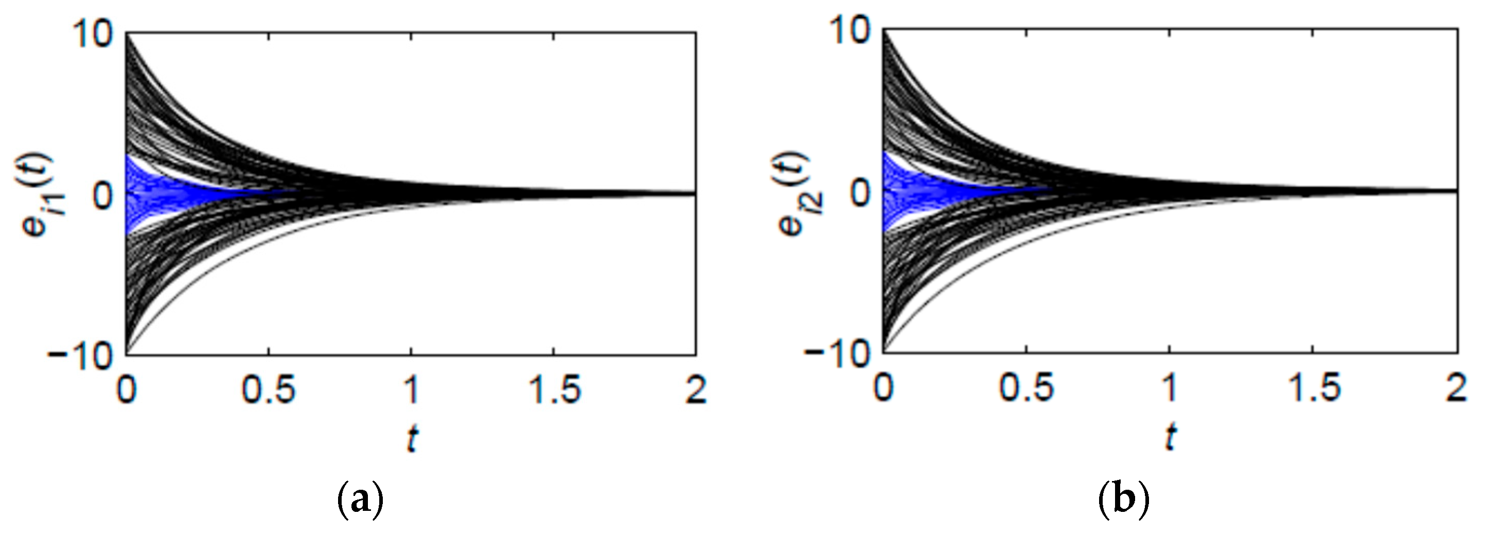
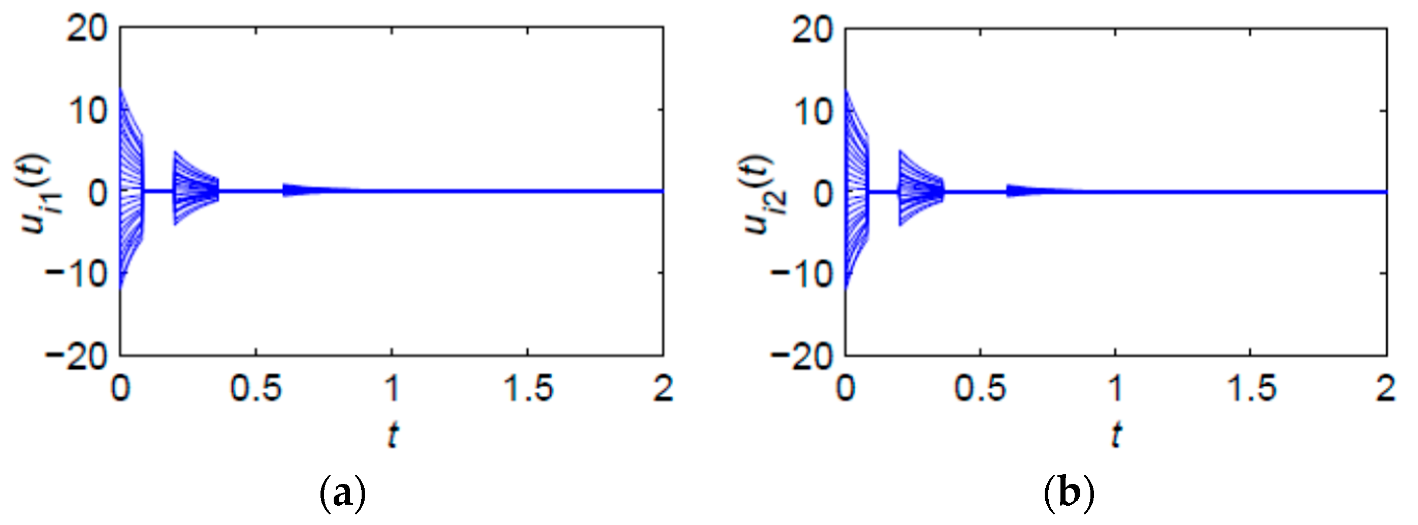
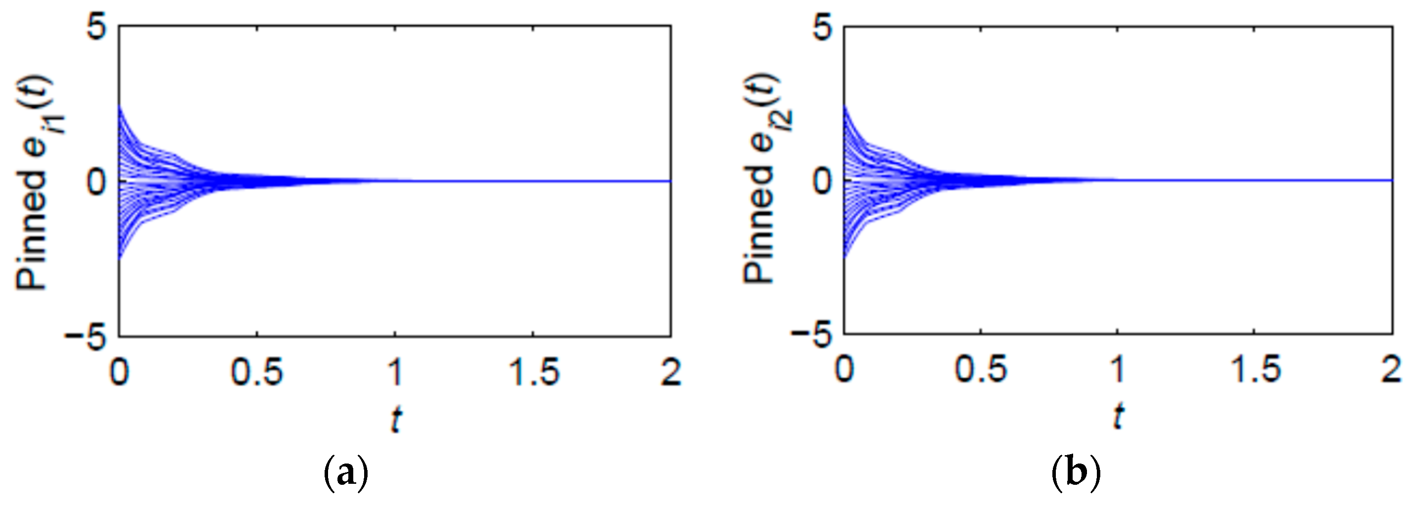
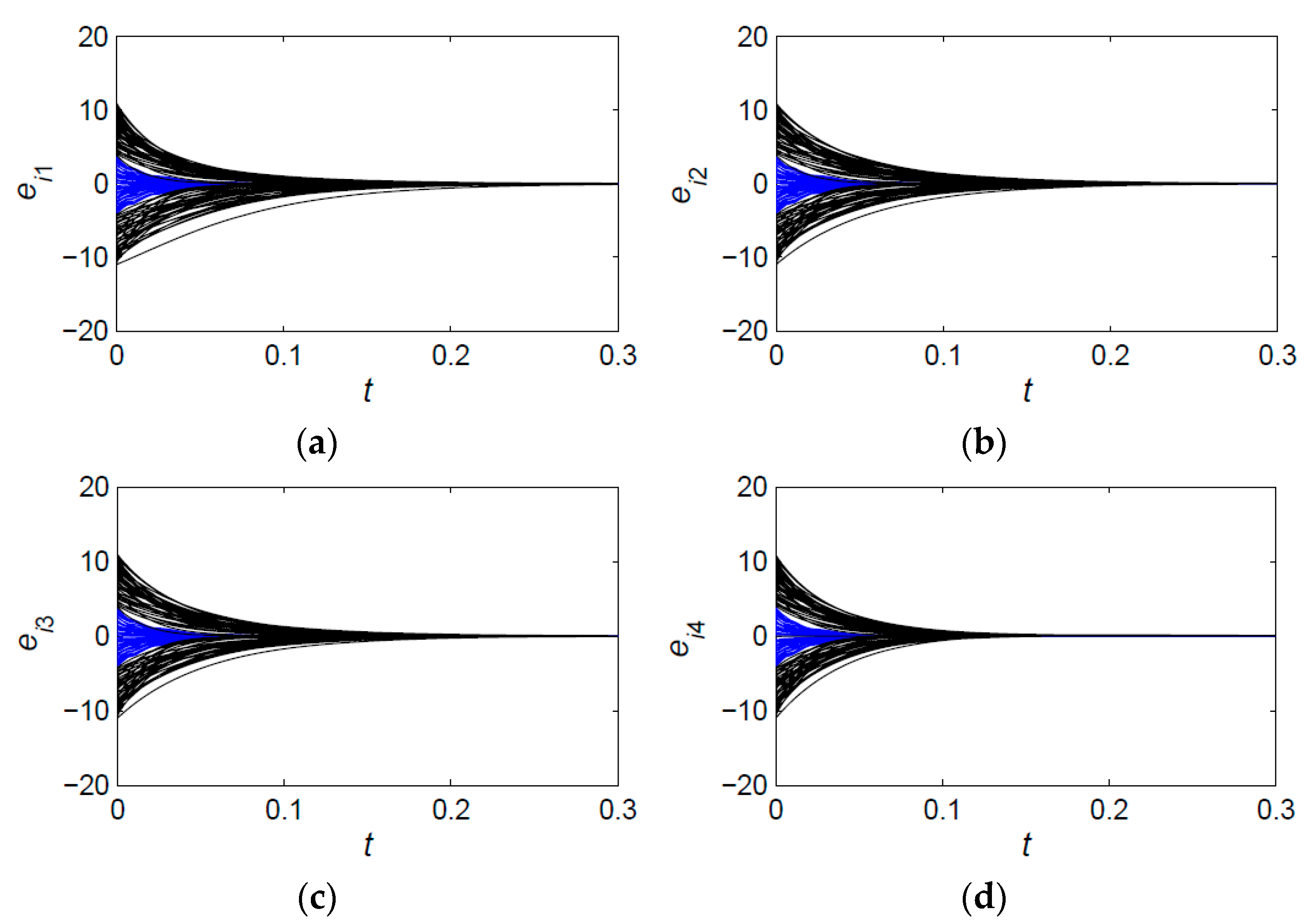
4. Simulation Examples

In order to illustrate the theoretical results, three numerical examples are introduced in this section.

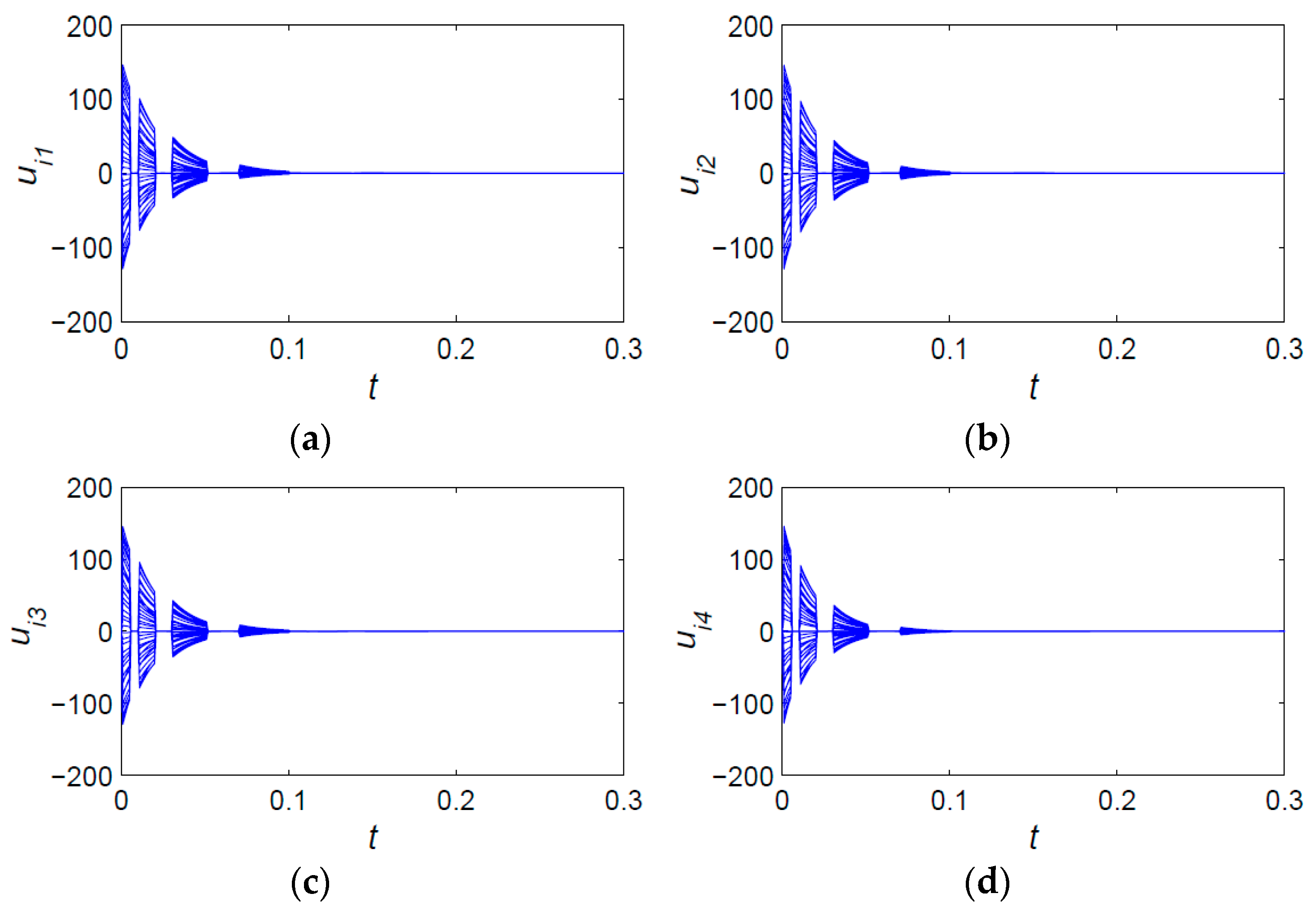
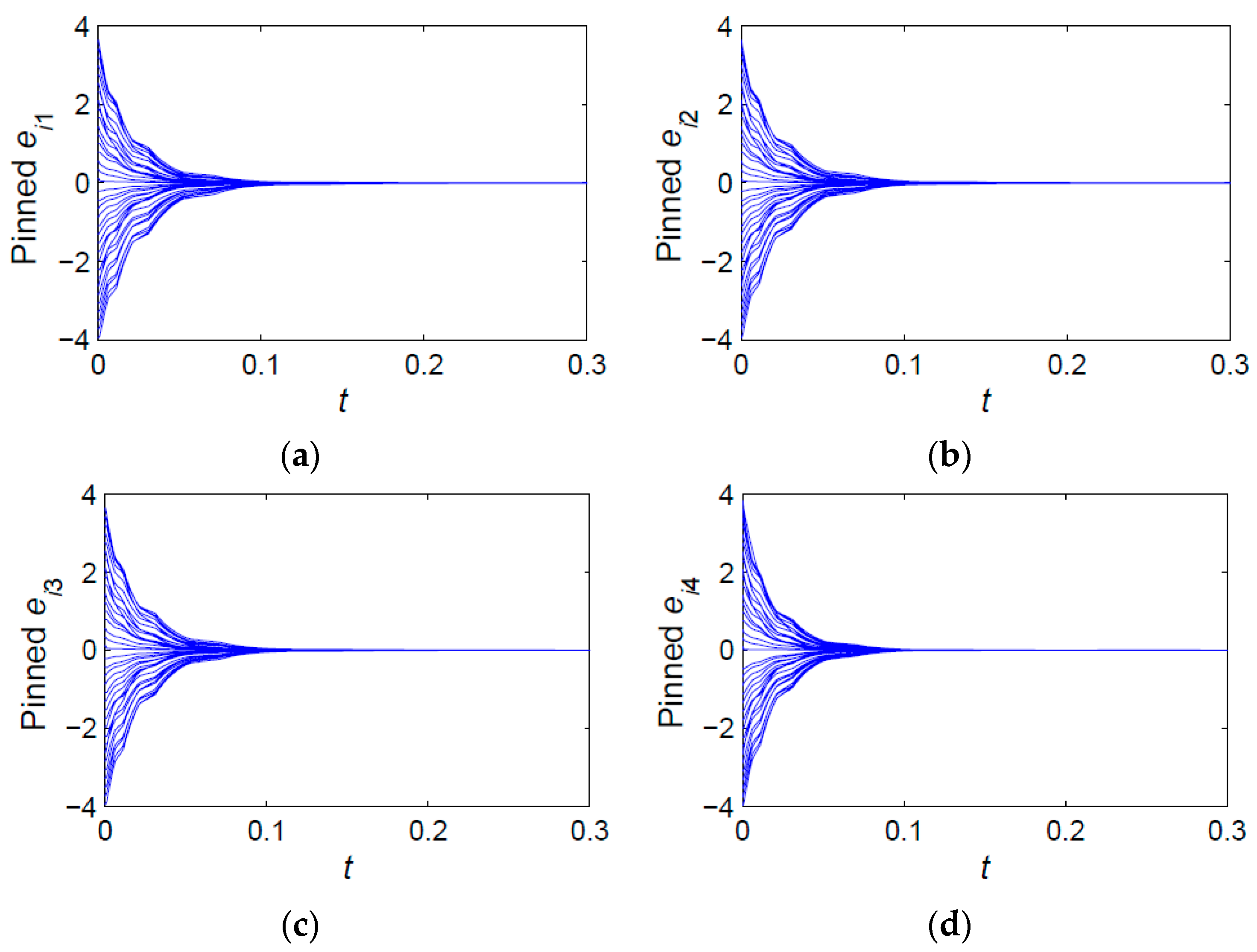
4.1. Simulation Example with State-Feedback Intermittent Pinning Controller

In this section, we give two simulation examples with a state-feedback intermittent pinning controller to verify the effectiveness of Theorem 1. Consider that each layer of two-layer complex networks has 100 nodes. The first layer is constructed by using a Watts–Strogatz small-world network with the initial degree m = 4 and the rewiring probability p = 0.3. The second layer is constructed as a Barabási–Albert scale-free network with initial nodes m₀ = 5. And for each layer, we use the random pinning strategy to generate its coupling matrix of networks.

4.1.1. Simulation Example 1

Consider the following dynamical system:

$$\left\{\begin{array}{l}{\dot{x}}_{i1}(t)=\frac{1}{q}sin(x_{i1}(t))\\ {\dot{x}}_{i2}(t)=con(\frac{1}{q}{x}_{i2}(t))\end{array}\right.,i=1,2,\dots ,100$$

(13)

where q is a non-zero real number. With a simple calculation, it can be obtained that $e_i^T(t)(f(y_i(t))-f(x_i(t)))\le$$\frac{1}{q}{e}_i^T(t)e_i(t)$. That is, $f(\cdot )$ satisfies the condition of Hypothesis 1, where $\rho =\frac{1}{q}$, $\Omega =I_2$. By choosing $q=5$, $D=I_2$, $c_1=c_2=0.2$, $l=25$, ${\gamma }_i=5$, $\overline{\omega }=1$, and $\overline{d}=1$, one has $\overline{\rho }=\rho =0.2$; a maximum eigenvalue for $(\overline{\rho }{I}_N+{\displaystyle \sum _{k=1}^2(c_k{A}^{(k)})-\Gamma )}$ is −0.312; a = 0.624 and b = 0.4. For $k\in \mathcal{N}$, when $-a{h}_k+b{\overline{h}}_k<0$($h_k\ge 1.56{\overline{h}}_k$), i.e., $\frac{h_k}{T_k}\ge 39.1\%$, $\underset{j\to \infty }{\lim }(-a({\displaystyle \sum _{k=0}^j{h}_k})+b({\displaystyle \sum _{k=0}^j{\overline{h}}_k}))=-\infty$ holds. Set $T_1=[0,0.2)$, $T_2=[0.2,0.6)$, $T_3=[0.6,1.6)$, $T_4=[1.6,2.4)$, …, and $\frac{h_k}{T_k}=40\%$; then, its corresponding control widths are $h_1=0.08$, $h_2=0.16$, $h_3=0.4$, $h_4=0.32$, … These parameters satisfy the conditions of Theorem 1. For the drive system (1) and the response system (2), we choose initial values $x_{i1}(0)=$ $0.01+0.1\times i\times {(-1)}^i$, $x_{i2}(0)=0.02+0.1\times i\times {(-1)}^i$, $y_{i1}(0)=0.01+0.2\times i\times {(-1)}^i$, and $y_{i2}(0)=0.02+$ $0.2\times i\times {(-1)}^i$, respectively. Under the controller (7), the system of differential equations is solved with the step size 0.001 by using the four-order Runge_Kutta method. Figure 1a,b shows evolution trends of synchronization error components of 100 nodes, where the blue curves represent error components of the pinned nodes. To show the effect of intermittent and pinning control, evolutions of the state-feedback intermittent pinning controller are shown in Figure 2a,b and Figure 3a,b, also displaying evolutions of error components of the pinned nodes (25 nodes).

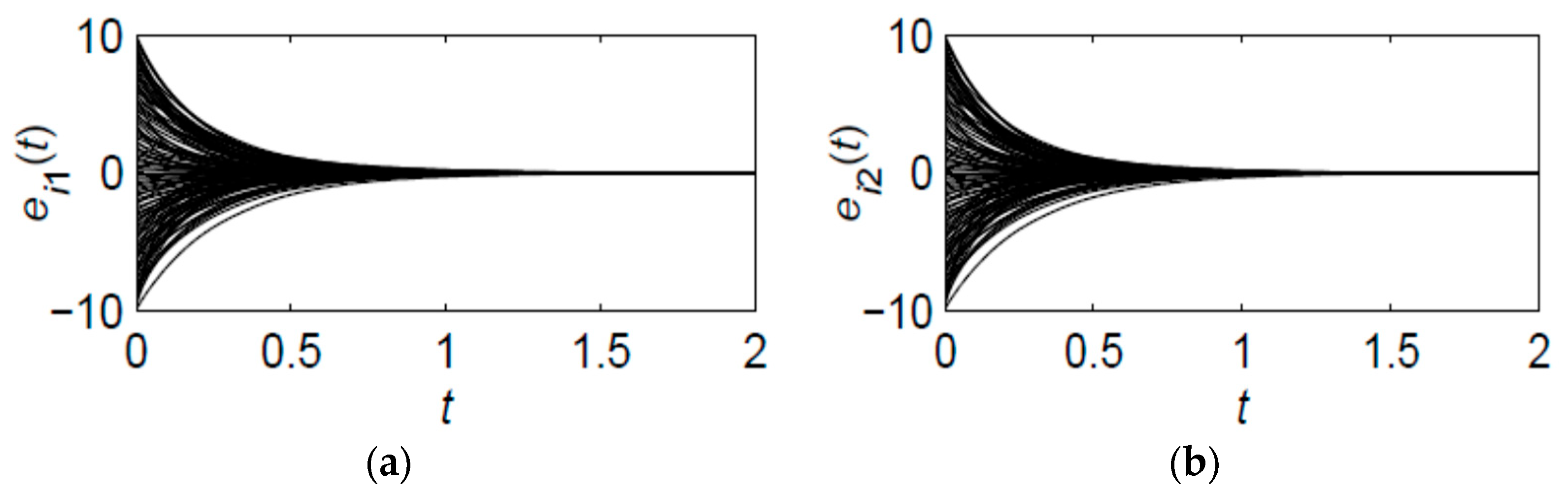
4.1.2. Simulation Example 2

In fact, the condition of the nonlinear functions satisfying Hypothesis 1 is weaker. Moreover, some chaotic systems also satisfy the above conditions, which include Lorenz system [39], Chua’s circuit [40], Lü system [41], hyperchaotic Sprott S system [42,43], and so on. Next, choose a hyperchaotic system to verify the adaptability of the control scheme. In this example, two two-layer complex networks still use network structures and parameters of simulation example 1 above.

The 4D hyperchaotic Sprott S system is as follows:

$$\left\{\begin{array}{l}{\dot{x}}_{i1}(t)=-x_{i1}(t)-4x_{i2}(t)\\ {\dot{x}}_{i2}(t)=x_{i1}(t)+x_{i3}^2(t)+a_1{x}_{i4}(t)\\ {\dot{x}}_{i3}(t)=1+x_{i1}(t)\\ {\dot{x}}_{i4}(t)=-a_2{x}_{i2}(t)\end{array}\right.,i=1,2,\dots ,100$$

(14)

from reference [42], with a₁ = 0.01, a₂ = 0.1, and $|x_{i1}(t)|<5$, $|x_{i2}(t)|<2.5$, $|x_{i3}(t)|<2$, the 4D Sprott S system exhibits a hyperchaotic attractor.

$$\begin{array}{l}{e}_i^T(t)(f(y_i(t))-f(x_i(t)))=(e_{i1}(t),e_{i2}(t),e_{i3}(t),e_{i4}(t))\left(\begin{array}{l}-e_{i1}(t)-4e_{i2}(t)\\ e_{i1}(t)+e_{i3}(t)(x_{i3}(t)+y_{i3}(t))+a_1{e}_{i4}(t)\\ e_{i1}(t)\\ -a_2{e}_{i2}(t)\end{array}\right)\\ \le -e_{i1}^2(t)+3|e_{i1}(t)e_{i2}(t)|+|e_{i1}(t)e_{i3}(t)|+4|e_{i2}(t)e_{i3}(t)|+|a_1-a_2|e_{i2}(t)e_{i4}(t)\\ \le (\frac{3}{2{\alpha }_1}+\frac{1}{2{\alpha }_2}-1)e_{i1}^2(t)+(\frac{3{\alpha }_1}{2}+\frac{2}{{\alpha }_3}+\frac{|a_1-a_2|}{2{\alpha }_4})e_{i2}^2(t)+(\frac{{\alpha }_2}{2}+2{\alpha }_3)e_{i3}^2(t)+\frac{|a_1-a_2|}{2}{\alpha }_4{e}_{i4}^2(t)\end{array}$$

where $e_i(t)={[e_{i1}(t),e_{i2}(t),e_{i3}(t),e_{i4}(t)]}^T$, $e_{ij}(t)=y_{ij}(t)-x_{ij}(t),j=1,2,3,4$, ${\alpha }_1$, ${\alpha }_2$, ${\alpha }_3$, and ${\alpha }_4$ are undetermined positive constants. Let ${\alpha }_1=\frac{1}{2}$, ${\alpha }_2=1$, ${\alpha }_3=1$, and ${\alpha }_4=20$, then $e_i^T(t)(f(y_i(t))-f(x_i(t)))<2.5e_{i1}^2(t)+3e_{i2}^2(t)+2.5e_{i3}^2(t)+e_{i4}^2(t)\le e_i^T(t)\Omega e_i(t)$. It is obvious that hyperchaotic system (14) satisfies Hypothesis 1, where $\rho =1$, $\Omega =$$diag(2.5,3,2.5,1)$. By choosing $D=diag(7.5,7.5,7.5,7.5)$, $c_1=c_2=0.2$, $l=35$, ${\gamma }_i=5$, $\overline{\omega }=3$, and $\overline{d}=7.5$, one obtains $\overline{\rho }=0.4$, a maximum eigenvalue for $(\overline{\rho }{I}_N+{\displaystyle \sum _{k=1}^2(c_k{A}^{(k)})-\Gamma )}=-0.3315$, a = 4.97, and b = 6. Therefore, when $-a{h}_k+b{\overline{h}}_k<0$, i.e., $\frac{h_k}{T_k}\ge 55\%$, $\underset{j\to \infty }{\lim }(-a({\displaystyle \sum _{k=0}^j{h}_k})+b({\displaystyle \sum _{k=0}^j{\overline{h}}_k}))=-\infty$ holds. Set $T_1=[0,0.01)$, $T_2=[0.01,0.03)$, $T_3=[0.03,0.07)$, $T_4=[0.07,0.13)$, $T_5=[0.13,0.2)$… By applying $\frac{h_k}{T_k}=55\%$, their corresponding control widths are $h_1=0.0055$, $h_2=0.011$, $h_3=0.022$, $h_4=0.033$, $h_5=0.0383$… For the drive system (1) and the response system (2), initial values are chosen as $x_{i1}(0)=0.13-0.1\times i\times {(-1)}^i$, $x_{i2}(0)=0.15-0.1\times i\times {(-1)}^i$, $x_{i3}(0)=0.15-0.1\times i\times {(-1)}^i$, $x_{i4}(0)=0.13-0.1\times i\times {(-1)}^i$, $y_{i1}(0)=0.02+0.01\times i\times {(-1)}^i$, $y_{i2}(0)=0.05+0.01\times i\times {(-1)}^i$, $y_{i3}(0)=0.05+0.01\times i\times {(-1)}^i$, and $y_{i4}(0)=0.05+0.01\times i\times {(-1)}^i$, respectively. Under the controller (7), differential equations are solved with the step size 0.001 by using the four-order Runge_Kutta method. Figure 4a–d shows evolution trends of error components of 100 nodes of the drive system and the response system, where synchronization errors tend to zeros. Figure 5a–d shows the effect of intermittent and pinning control of four controllers. Evolutions of error components of the pinned nodes (35 nodes) were drawn in Figure 6a–d.

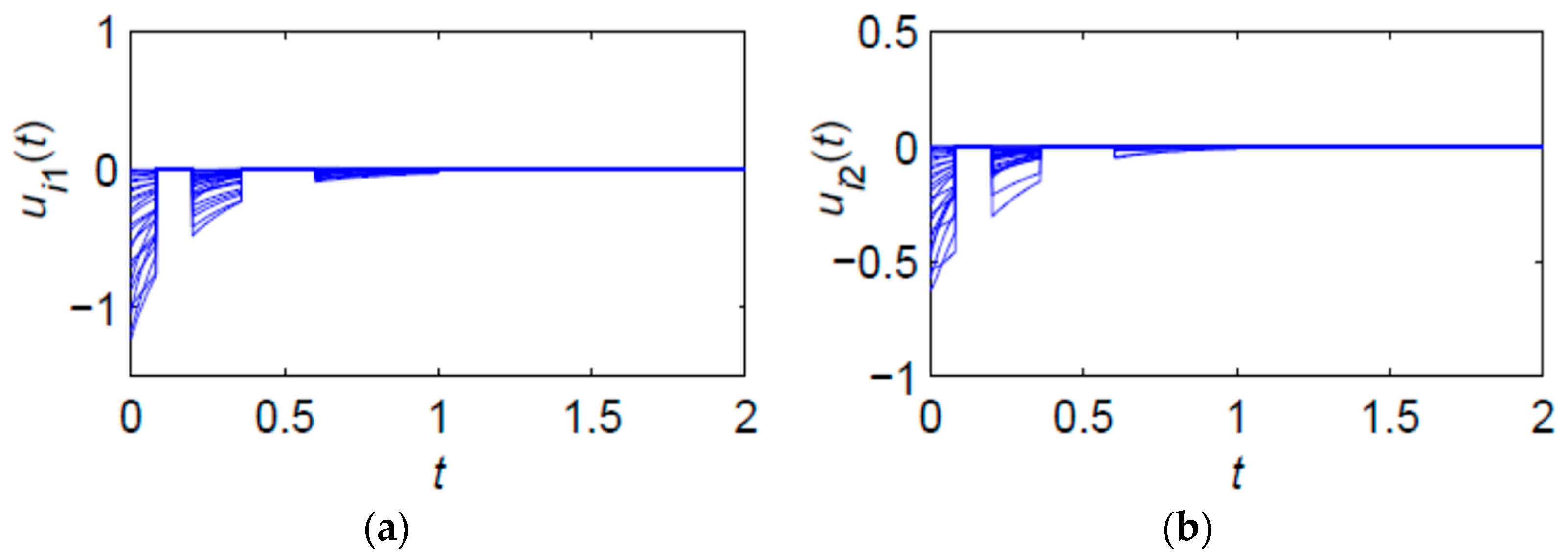
4.2. Simulation Example with Adaptive Intermittent Pinning Controller

In this numerical example, in order to compare the simulation effect with linear feedback control, the same network structures, dynamic system, and related parameters are chosen as the above simulation example 1. The first and second layers of networks are, respectively, a small-world network and scale-free network with 100 nodes. The parameters generating networks are the same as the above, and random pinning control strategy is used. The node nonlinear dynamic system is the same as the above example 1, clearly satisfying Hypothesis 1. Let $\Omega =I_2$, $D=I_2$, $c_1=c_2=0.2$, $l=25$, ${\epsilon }_i=5,1\le i\le 25$, $\overline{\omega }=1$, and $\overline{d}=1$, which yields $\overline{\rho }=\rho =0.2$; a maximum eigenvalue for $(\overline{\rho }{I}_N+{\displaystyle \sum _{k=1}^2(c_k{A}^{(k)})-\epsilon I_{Nl})}$ is 0.312, and $\overline{a}=0.624$, $\overline{b}=0.4$. When $\frac{h_k}{T_k}\ge 39.1\%$, $\underset{j\to \infty }{\lim }(-\overline{a}({\displaystyle \sum _{k=0}^j{h}_k})+\overline{b}({\displaystyle \sum _{k=0}^j{\overline{h}}_k}))=-\infty$ holds. Similarly, intermittent time slots are chosen as $T_1=[0,0.2)$, $T_2=[0.2,0,6)$, $T_3=[0.6,1.6)$, $T_4=[1.6,2.4)$,…; then, corresponding control widths are $h_1=0.08$, $h_2=0.16$, $h_3=0.4$, $h_4=0.32$, … Initial values of drive-response systems are respectively chosen as $x_{i1}(0)=0.02+0.1\times i\times {(-1)}^i$, $x_{i2}(0)=0.01+0.1\times i\times {(-1)}^i$, $y_{i1}(0)=0.01+0.2\times i\times {(-1)}^i$, and $y_{i2}(0)=0.02+0.2\times i\times {(-1)}^i$. Under the adaptive controller in Equation (10), evolution trends of synchronization errors are shown in Figure 7. Figure 8 shows evolution trends of the adaptive intermittent pinning controller. Lastly, evolution trends of adaptive control gain components were drawn in Figure 9.

From the simulation examples mentioned above, it can be seen that synchronization speed with an adaptive intermittent pinning controller is faster than that with a state-feedback intermittent pinning controller, and its pinning control effort is weaker.

5. Conclusions

In this paper, by using pinning and aperiodically intermittent controllers, we study the outer synchronization problem of two multi-layer dynamical networks with additive couplings, and the outer synchronization models of networks do not involve system delay and transmission delay. The sufficient conditions are obtained to ensure the synchronization of multi-layer networks under the state-feedback intermittent pinning controller and the adaptive intermittent pinning controller, respectively. Finally, from simulation examples, it can be observed that two multi-layer networks with two different control methods and different dynamical systems can achieve outer synchronization. In particular, three simulation examples show the intermittent and pinning control effect of control schemes.

References

1. Arenas, A.; Díaz-Guilera, A.; Kurths, J.; Moreno, Y.; Zhoug, C. Synchronization in complex networks. Phys. Rep. 2008, 469, 93–153. [Google Scholar] [CrossRef]
2. Zhu, J.; Lu, J.; Yu, X. Flocking of Multi-Agent Non-Holonomic Systems with Proximity Graphs. IEEE Trans. Circuits Syst. I 2013, 60, 199–210. [Google Scholar] [CrossRef]
3. Xie, Q.; Chen, G.; Bollt, E. Hybrid chaos synchronization and its application in information processing. Math. Comput. Model. 2002, 35, 145–163. [Google Scholar] [CrossRef]
4. Wang, P.; Lü, J.; Ogorzalek, M.J. Global relative parameter sensitivities of the feed-forward loops in genetic networks. Neurocomputing 2012, 78, 155–165. [Google Scholar] [CrossRef]
5. Tang, Y.; Qian, F.; Gao, H.; Kurths, J. Synchronization in complex networks and its application—A survey of recent advances and challenges. Annu. Rev. Control 2014, 38, 184–198. [Google Scholar] [CrossRef]
6. Zhao, L.-H.; Wen, S.; Li, C.; Shi, K.; Huang, T. A Recent Survey on Control for Synchronization and Passivity of Complex Networks. IEEE Trans. Netw. Sci. Eng. 2022, 9, 4235–4254. [Google Scholar] [CrossRef]
7. Boccaletti, S.; Bianconi, G.; Criado, R.; del Genio, C.; Gómez-Gardeñes, J.; Romance, M.; Sendiña-Nadal, I.; Wang, Z.; Zanin, M. The structure and dynamics of multilayer networks. Phys. Rep. 2014, 544, 1–122. [Google Scholar] [CrossRef]
8. Tang, L.; Wu, X.; Lü, J.; Lu, J.; Raissa, M.D. Master stability functions for complete, intralayer and interlayer synchronization in multiplex networks of coupled Rossler oscillators. Phys. Rev. E 2019, 99, 012304. [Google Scholar] [CrossRef]
9. Tang, L.; Lu, J.; Lü, J. A threshold effect of coupling delays on intra-layer synchronization in duplex networks. Sci. China-Technol. Sci. 2018, 61, 1907–1914. [Google Scholar] [CrossRef]
10. Bera, B.K.; Rakshit, S.; Ghosh, D. Intralayer synchronization in neuronal multiplex network. Eur. Phys. J. Spec. Top. 2019, 228, 2441–2454. [Google Scholar] [CrossRef]
11. Kivela, M.; Arenas, A.; Barthelemy, M. Multilayer networks. J. Complex Netw. 2014, 2, 203–271. [Google Scholar] [CrossRef]
12. Wang, G.; Cao, J.; Lu, J. Outer synchronization between two nonidentical networks with circumstance noise. Phys. A Stat. Mech. Appl. 2010, 389, 1480–1488. [Google Scholar] [CrossRef]
13. Hymavathi, M.; Ibrahim, T.F.; Syed Ali, M.; Stamov, G.; Stamova, I.; Younis, B.A.; Osman, K.I. Synchronization of fractional-order neural networks with time delays and reaction-diffusion terms via pinning control. Mathematics 2022, 10, 3916. [Google Scholar] [CrossRef]
14. Zhuang, J.; Zhou, Y.; Xia, Y. Synchronization analysis of drive-response multi-layer dynamical networks with additive couplings and stochastic perturbations. Discret. Contin. Dyn. Syst. S 2021, 14, 1607–1629. [Google Scholar] [CrossRef]
15. Żochowski, M. Intermittent dynamical control. Phys. D Nonlinear Phenom. 2000, 145, 181–190. [Google Scholar] [CrossRef]
16. Xia, W.; Cao, J. Pinning synchronization of delayed dynamical networks via periodically intermittent control. Chaos Interdiscip. J. Nonlinear Sci. 2009, 19, 013120. [Google Scholar] [CrossRef] [PubMed]
17. Cai, S.; Hao, J.; He, Q.; Liu, Z. Exponential synchronization of complex delayed dynamical networks via pinning periodically intermittent control. Phys. Lett. A 2011, 375, 1965–1971. [Google Scholar] [CrossRef]
18. Hu, C.; Yu, J.; Jiang, H.; Teng, Z. Exponential Synchronization of Complex Networks with Finite Distributed Delays Coupling. IEEE Trans. Neural Netw. 2011, 22, 1999–2010. [Google Scholar] [CrossRef] [PubMed]
19. Liang, Y.; Wang, X. Synchronization in complex networks with non-delay and delay couplings via intermittent control with two switched periods. Phys. A Stat. Mech. Its Appl. 2013, 395, 434–444. [Google Scholar] [CrossRef]
20. Liang, Y.; Qi, X.; Wei, Q. Synchronization of delayed complex networks via intermittent control with non-period. Phys. A Stat. Mech. Its Appl. 2018, 492, 1327–1339. [Google Scholar] [CrossRef]
21. Li, W.; Zhou, J.; Li, J.; Xie, T.; Lu, J.-A. Cluster Synchronization of Two-Layer Networks via Aperiodically Intermittent Pinning Control. IEEE Trans. Circuits Syst. II Express Briefs 2021, 68, 1338–1342. [Google Scholar] [CrossRef]
22. Jing, T.; Zhang, D.; Zhang, X. New Criteria for Synchronization of Multilayer Neural Networks via Aperiodically Intermittent Control. Comput. Intell. Neurosci. 2022, 2022, 8157794. [Google Scholar] [CrossRef]
23. Yang, H.; Wang, X.; Zhong, S.; Shu, L. Synchronization of nonlinear complex dynamical systems via delayed impulsive distributed control. Appl. Math. Comput. 2018, 320, 75–85. [Google Scholar] [CrossRef]
24. Zhuang, J.; Zhou, Y.; Xia, Y. Intra-layer synchronization in duplex networks with time-varying delays and stochastic perturba-tions under impulsive control. Neural Process. Lett. 2021, 52, 785–804. [Google Scholar] [CrossRef]
25. Liu, X.; Fu, H.; Liu, L. Leader-Following Mean Square Consensus of Stochastic Multi-agent Systems via Periodically Intermittent Event-Triggered Control. Neural Process. Lett. 2020, 53, 275–298. [Google Scholar] [CrossRef]
26. Zhang, C.; Zhang, C.; Meng, F.W.; Liang, Y. Event-Triggered Control for In-tra/Inter-Layer Synchronization and Quasi-Synchronization in Two-Layer Coupled Networks. Mathematics 2023, 11, 1458. [Google Scholar] [CrossRef]
27. Zhang, C.; Zhang, C.; Zhang, X.; Wang, F.; Liang, Y. Dynamic event-triggered control for intra/inter-layer synchronization in multi-layer networks. Commun. Nonlinear Sci. Numer. Simul. 2023, 119, 107124. [Google Scholar] [CrossRef]
28. Wang, X.F.; Chen, G. Pinning control of scale-free dynamical networks. Phys. A Stat. Mech. Appl. 2002, 310, 521–531. [Google Scholar] [CrossRef]
29. Porfiri, M.; Bernardo, M.D. Criteria for global pinning-controllability of complex networks. Automatica 2008, 44, 3100–3106. [Google Scholar] [CrossRef]
30. Yu, W.; Chen, G.; Lü, J.; Kurths, J.; Yu, G.C.W.; Jin, S.; Wang, D.; Zou, X.; Yan, F.; Gu, G.; et al. Synchronization via Pinning Control on General Complex Networks. SIAM J. Control Optim. 2013, 51, 1395–1416. [Google Scholar] [CrossRef]
31. Zhao, X.; Zhou, J.; Lu, J.-A. Pinning Synchronization of Multiplex Delayed Networks with Stochastic Perturbations. IEEE Trans. Cybern. 2019, 49, 4262–4270. [Google Scholar] [CrossRef] [PubMed]
32. Hai, X.; Ren, G.; Yu, Y.; Xu, C. Adaptive Pinning Synchronization of Fractional Complex Networks with Impulses and Reaction–Diffusion Terms. Mathematics 2019, 7, 405. [Google Scholar] [CrossRef]
33. Jin, X.; Wang, Z.; Yang, H.; Song, Q.; Xiao, M. Synchronization of multiplex networks with stochastic perturbations via pinning adaptive control. J. Frankl. Inst. 2021, 358, 3994–4012. [Google Scholar] [CrossRef]
34. He, W.; Chen, G.; Han, Q.-L.; Du, W.; Cao, J.; Qian, F. Multiagent Systems on Multilayer Networks: Synchronization Analysis and Network Design. IEEE Trans. Syst. Man Cybern. Syst. 2017, 47, 1655–1667. [Google Scholar] [CrossRef]
35. Zhuang, J.; Cao, J.; Tang, L.; Xia, Y.; Perc, M. Synchronization Analysis for Stochastic Delayed Multilayer Network with Additive Couplings. IEEE Trans. Syst. Man Cybern. Syst. 2020, 50, 4807–4816. [Google Scholar] [CrossRef]
36. Zhang, F. Matrix Theory; Springer: New York, NY, USA, 1999. [Google Scholar]
37. Lütkepohl, H. Handbook of Matrices; Wiley: New York, NY, USA, 1996. [Google Scholar]
38. Liang, Y.; Wang, X. A method of quickly calculating the number of pinning nodes on pinning synchronization in complex networks. Appl. Math. Comput. 2014, 246, 743–751. [Google Scholar] [CrossRef]
39. Lorenz, E.N. Deterministic nonperiodic flow. J. Atmos. Sci. 1963, 20, 130–141. [Google Scholar] [CrossRef]
40. Matsumoto, T. A chaotic attractor from Chua’s circuit. IEEE Trans. Circuits Syst. 1984, 31, 1055–1058. [Google Scholar] [CrossRef]
41. Lü, J.; Chen, G. A new chaotic attractor coined. Int. J. Bifurc. Chaos 2002, 12, 659–661. [Google Scholar] [CrossRef]
42. Al-Hayali, M.A.; Al-Azzawi, F.S. A 4D hyperchaotic Sprott S system with multistability and hidden attractors. J. Phys. Conf. Ser. 2021, 1879, 032031. [Google Scholar] [CrossRef]
43. Nadia, M.M.; Zeena, N.A. A new secure encryption algorithm based on RC4 cipher and 4D hyperchaotic Sprott-S system. In Proceedings of the 5th College of science International Conference on Recent Trends in Information Technology, Baghdad, Iraq, 15–16 November 2022. [Google Scholar] [CrossRef]
Figure 1. Evolution trends of synchronization errors of two-layer network with 100 nodes, where the blue curves represent error components of the pinned nodes (25 nodes). (a) Error components e i 1 ( t ) . (b) Error components e i 2 ( t ) , i = 1 , 2 , , 25 .
Mathematics 11 03543 g001
Figure 2. Evolution trends of the intermittent pinning controller. (a) Controller components u i 1 ( t ) . (b) Controller components u i 2 ( t ) , i = 1 , 2 , , 25 .
Mathematics 11 03543 g002
Figure 3. Evolution trends of pinned node errors. (a) Time evolution of error components e i 1 ( t ) . (b) Time evolution of error components e i 2 ( t ) , i = 1 , 2 , , 25 .
Mathematics 11 03543 g003
Figure 4. Evolution trends of synchronization errors of two-layer network with 100 nodes, where the blue curves represent error components of the pinned nodes (35 nodes). (a) Error components e i 1 ( t ) . (b) Error components e i 2 ( t ) . (c) Error components e i 2 ( t ) . (d) Error components e i 4 ( t ) , i = 1 , 2 , , 100 .
Mathematics 11 03543 g004
Figure 5. Evolution trends of the intermittent pinning controller. (a) Controller components u i 1 ( t ) . (b) Controller components u i 2 ( t ) . (c) Controller components u i 3 ( t ) . (d) Controller components u i 4 ( t ) , i = 1 , 2 , , 35 .
Mathematics 11 03543 g005
Figure 6. Evolution trends of pinned node errors. (a) Time evolution of error components e i 1 ( t ) . (b) Time evolution of error components e i 2 ( t ) . (c) Time evolution of error components e i 3 ( t ) . (d) Time evolution of error components e i 4 ( t ) , i = 1 , 2 , , 35 .
Mathematics 11 03543 g006
Figure 7. Evolution trends of synchronization errors of two-layer network with 100 nodes, where the blue curves represent error components of the pinned nodes (25 nodes). (a) Error components e i 1 ( t ) . (b) Error components e i 2 ( t ) , i = 1 , 2 , , 100 .
Mathematics 11 03543 g007
Figure 8. Evolution trends of the adaptive intermittent pinning controller. (a) Controller components u i 1 t . (b) Controller components u i 2 ( t ) , i = 1 , 2 , , 25 .
Mathematics 11 03543 g008
Figure 9. Evolution trends of the adaptive control gains. (a) Control gain components γ i 1 ( t ) . (b) Control gain components γ i 2 ( t ) , i = 1 , 2 , , 25 .
Mathematics 11 03543 g009
Disclaimer/Publisher’s Note: The statements, opinions and data contained in all publications are solely those of the individual author(s) and contributor(s) and not of MDPI and/or the editor(s). MDPI and/or the editor(s) disclaim responsibility for any injury to people or property resulting from any ideas, methods, instructions or products referred to in the content.