Generating Robust Optimal Mixture Designs Due to Missing Observation Using a Multi-Objective Genetic Algorithm

Abstract

Missing observation is a common problem in scientific and industrial experiments, particularly in a small-scale experiment. They often present significant challenges when experiment repetition is infeasible. In this research, we propose a multi-objective genetic algorithm as a practical alternative for generating optimal mixture designs that remain robust in the face of missing observation. Our algorithm prioritizes designs that exhibit superior D-efficiency while maintaining a high minimum D-efficiency due to missing observations. The focus on D-efficiency stems from its ability to minimize the impact of missing observations on parameter estimates, ensure reliability across the experimental space, and maximize the utility of available data. We study problems with three mixture components where the experimental region is an irregularly shaped polyhedral within the simplex. Our designs have proven to be D-optimal designs, demonstrating exceptional performance in terms of D-efficiency and robustness to missing observations. We provide a well-distributed set of optimal designs derived from the Pareto front, enabling experimenters to select the most suitable design based on their priorities using the desirability function.

1. Introduction

Response surface methodology (RSM) is a collection of statistical and mathematical techniques utilized to develop new processes, enhance formulations, and optimize process performance. A mixture experiment is a special case of a response surface experiment, in which the components of the mixture cannot vary independently because their proportions must sum-up to a constant. The primary goal of a mixture design is to determine the optimal component proportion settings that maximize, minimize, or specify the response. Mixture experiments are frequently encountered in industries where product formulation is required, such as food and beverage processing, cosmetics, glass manufacturing, pharmaceutical drug production, cement production, polymer production and so on. For a detailed description of response surface methodology and mixture experiments, see Cornell [1] and Myers et al. [2].

In real-world situations, carefully planned experiments may encounter issues such as the failure to observe, the loss of responses for one or more runs during data collection, or dubious responses in certain circumstances, leading to missing observations. Responses or observations may be absent or unobservable for a variety of reasons. For instance, certain combinations of factors might create unstable conditions, resulting in implausible responses in chemical or biotechnical processes. Malfunctions or failures in equipment may lead to the destruction of some experimental units, thereby rendering the response unmeasurable. Additionally, in industrial experiments, responses may be unattainable or difficult to replicate at a design point due to extraneous factors often unrelated to the basic design structure, such as cost constraints, inefficiencies in time, technical unsatisfactoriness, transit issues, or other factors. The types of missing observations previously mentioned are commonly encountered during experiments aimed at developing new products. The absence of responses negatively impacts statistical analysis results, specifically, the quality of the regression coefficient estimates, resulting in a poorly fitting model. Box and Draper [3] and Myers et al. [2] suggested that an experimental design should be robust against missing observation. Therefore, it is crucial to develop such robust designs.

In the field of experimental design, the robustness of a design in the face of missing observations has been extensively studied, with a multitude of criteria and measures being proposed to assess this robustness. Box and Draper [3] explored how outliers, or wild observations, affect fitted values as obtained via least squares estimation in central composite designs. They also examined the relationship between the diagonal elements of the hat-matrix, $\mathit{H}$, and the robustness of a design. Taking a different perspective, Herzberg and Andrews [4] introduced the concept of design breakdown probability and proposed both generalized variance and minimization of the maximum variance criteria as measures of expected precision for assessing design robustness. Later, Andrews and Herzberg [5] demonstrated how to easily calculate this expected precision and proposed the average precision criterion based on the determinant of the information matrix to evaluate design robustness to missing observations. Akhtar and Prescott [6] studied the effect of missing observations in central composite designs and developed a minimax loss criterion for missing observations based on the D-optimality criterion.

Numerous researchers have attempted to develop various algorithms to construct designs that remain robust in the face of missing data. The minimax loss criterion, a popular tool, is frequently used for generating such robust designs. Ahmad et al. [7] constructed augmented pairs minimax loss designs using the minimax loss criterion and assessed the impact of missing observations through a loss function criterion proposed by Akhtar and Prescott [6]. Ahmad and Akhtar [8] constructed the new second-order response surface designs, known as repaired resolution central composite designs, that are robust to missing observations under the minimax loss criterion. Chen et al. [9] suggested orthogonal-array-based composite minimax loss designs that are robust to missing data, considering D-efficiency and generalized scaled standard deviation for near-saturated, saturated, or supersaturated designs. Alrweili et al. [10] constructed minimax loss response surface designs, demonstrating robustness against missing design points in terms of the minimax loss criterion. Oladugba and Nwanonobi [11] constructed definitive screening composite minimax loss designs, demonstrating robustness to missing observations in terms of D-efficiency and generalized scaled standard deviation. Yankam and Oladugba [12] developed orthogonal uniform minimax loss (OUCM) designs, finding that the OUCM design outperforms the loss criterion and displays higher D-efficiency, A-efficiency, and T-efficiency. In addition to the minimax loss criterion, da Silva et al. [13] proposed exchange algorithms to generate optimal designs that satisfy the compound criteria. They incorporated leverage uniformity into the compound design criterion and used a compound criterion to identify designs that are robust to missing runs when fitting a second-order model. Smucker et al. [14] introduced the truncated Herzberg–Andrews criterion to construct designs that perform comparably or better than classical designs when observations are missing.

The Genetic Algorithm (GA) is widely recognized as one of the most popular metaheuristic algorithms for optimizing complex solution spaces. It has proven effective in generating high-quality solutions for various optimization problems. Several researchers have utilized genetic algorithms to generate optimal designs based on a single objective function. For instance, Borkowski [15] employed a genetic algorithm to generate near-optimal D, A, G, and IV exact-point response surface designs for the second-order model in a hypercube. Concurrently, Heredia-Langner et al. [16] proposed a genetic algorithm for generating D-optimal designs in factorial regions and mixture problems, demonstrating that the performance of the genetic algorithm was on par with other procedures. Building on their previous work, Heredia-Langner et al. [17] used a genetic algorithm to generate model-robust optimal designs, optimizing a desirability function of D- or I-optimality criteria for a given set of potential models. In a scenario where the experimental budget or cost is limited, Park et al. [18] applied a genetic algorithm to generate cost-constrained G-efficient designs over a cuboidal region. Limmun et al. [19] developed a genetic algorithm to generate optimal designs based on the weighted A-criterion in mixture experiments, and later, they proposed a genetic algorithm to generate optimal designs using a weighted criterion based on the geometric mean in mixture experiments [20]. Mahachaichanakul and Srisuradetchai [21] proposed a genetic algorithm to construct D- and G-optimal robust response surface designs that were robust against missing observation.

Many well-known researchers have primarily focused on studying multi-objective genetic algorithms in engineering and scientific problems. Srinivas and Deb [22] were the first to introduce the Non-Dominating Sorting Genetic Algorithm (NSGA). Later, Deb et al. [23] introduced NSGA-II, an extended version of the NSGA. This algorithm proposed a fast nondominated sorting approach, along with the concept of crowding distance. It efficiently categorizes solutions into different Pareto fronts based on their dominance relationships and considers crowding distance as a secondary sorting criterion within each front. Long et al. [24] proposed a ranking strategy to enhance multi-objective genetic algorithms by improving the selection operator’s performance in finding solutions along the Pareto front. Furthermore, although several researchers have focused on studying multi-objective optimal design, they have not used genetic algorithms. Cook and Wong [25] explored the relationship between constrained and compound optimal design with multiple objectives. They investigated the conditions under which these two types of designs were equivalent. Zhang et al. [26] presented a methodology for constructing dual-objective optimal designs in mixture experiments within a simplex experimental region. They considered two types of dual-objectives: D- and A-optimality, and D- and I-optimality. Lu et al. [27] introduced a focused Pareto-front search algorithm, identifying the best non-dominated solutions based on multiple criteria with a preference for a more focused weighting space. This approach prioritizes objectively superior solutions before considering subjective user priorities. However, the literature appears to lack a comprehensive exploration of multi-objective genetic algorithms in the context of generating optimal designs for mixture experiments.

The primary aim of this research was to address a significant gap in the literature regarding the application of multi-objective genetic algorithms for generating robust optimal mixture designs, especially in the context of missing observations. The major contributions of this paper are as follows:

• We proposed the use of multi-objective genetic algorithms to generate robust optimal mixture designs due to missing observation. In situations where a single missing observation is inevitable in an experiment, experimenters still need a design that remains robust against this absence, especially in smaller experimental settings. Our goal here is to generate designs robust against missing observations in small experiments using a genetic algorithm. These designs aim to preserve not just commendable D-efficiency, but also maintain a favorable minimum D-efficiency due to missing observations;
• We conducted a comparative assessment of our GA and NSGA-II based on both qualitative and quantitative performance metrics. To ensure fair evaluations of these competing methodologies, we adopted the same genetic operator and genetic algorithm parameters but employed distinct selection processes. Specifically, the NSGA approach incorporated non-dominated sorting, crowding distance, and tournament selection, whereas our GA approach combined non-dominated sorting with random pair selection;
• This paper proposed the concept of how to assess the robustness of designs in the face of missing observations. We evaluated the robustness due to missing observation of GA designs (as generated using our GA), NSGA designs (as generated using NSGA-II), and DX designs (as generated using Design-Expert 11 software);
• We also introduced the concept of how to select the optimal mixture design based on alignment with experimental priorities and considering the trade-offs between the two objective functions.

The remainder of this paper is organized into nine sections. Section 2 provides a theoretical background of our research. The loss of efficiency in terms of the optimality criteria is explored in Section 3. Our genetic algorithm, designed to address these multi-objective functions, is presented in Section 4. Section 5 outlines the methodology for examining the performance of the designs. Section 6 presents two illustrative experiments that demonstrate the performance of the proposed algorithm. Finally, Section 7 provides the conclusions and suggestions for future work directions.

2. Theoretical Background

2.1. Notation and Model

In a mixture experiment, the number of ingredients (components) is denoted by $q$, and the proportion of each ingredient (component) is represented by $x_1,x_2,\dots ,x_q$. The response variable in a mixture experiment depends solely on the relative proportions of the components. A defining characteristic of standard mixture experiments is that

$$0\le x_i\le 1 \mathrm{a}\mathrm{n}\mathrm{d} \sum _{i=1}^q{x}_i=1.$$

(1)

These restrictions remove a degree of freedom from the component proportions and then each $x_i$ can only lie inside a $(q-1)$-dimensional regular simplex. The lower ($L_i)$ and/or upper $\left(U_i\right)$ bound constraints are commonly applied to the component proportions, which are referred to as single-component constraints (SCCs). The SCCs are expressed as

$$0\le L_i\le x_i\le U_i\le 1 \mathrm{for} i=1, 2, \dots , q.$$

(2)

Moreover, the linear multiple-component constraints (MCCs) are frequently found among the proportions of the form’s components and are expressed as

$$C_j\le \sum _{i=1}^q{A}_{ij}{x}_i\le D_j;j=1, 2, \dots , h,$$

(3)

where $A_{ij}$ are constants defining multivariate linear with $C_j$ and $D_j$ being the lower and upper bounds of the MCCs, respectively. In addition, the nonlinear multicomponent constraints are also possible, but they are less common and seldom addressed in the theoretical literature. If the single-component constraints (SCCs) and/or multiple-component constraints (MCCs) are imposed on the component proportions, the experimental region of interest changes from a simplex to an irregularly shaped polyhedron within the simplex. For a detailed review of mixture experiments, see Cornell [1] and Myers et al. [2].

There is a wide range of potential models that can be employed in mixture experiments. The Scheffé models are most commonly used for data derived from mixture experiments because of their ability to handle the natural restrictions in mixture experiments. The Scheffé mixture models include all components in the model and do not contain an intercept term due to the constraints on component proportions. In a mixture experiment with $q$-components $(x_i; i=1, 2, \dots , q)$, the Scheffé linear mixture model has the form

$$y=\sum _{i=1}^q{\beta }_i{x}_i+\epsilon ,$$

(4)

and the Scheffé quadratic mixture model can be expressed as

$$y=\sum _{i=1}^q{\beta }_i{x}_i+\sum _{i=1}^{q-1}\sum _{j=i+1}^q{\beta }_{ij}{x}_i{x}_j+\epsilon ,$$

(5)

where $y$ represents the measured response variable; the coefficient ${\beta }_i$ represents the expected response to the $i$th pure component; the coefficient ${\beta }_{ij}$ represents the nonlinear blending between the $i$th and the $j$th components; and $\epsilon$ represents the error term accounting for random error. The error term is assumed to be independently and identically distributed as $N(0,{\sigma }^2)$.

In this research, we make the assumption that the experimenter believes that the Scheffé quadratic mixture model can adequately approximate the true model. In matrix notation, the Scheffé mixture model can be written as

$$\mathit{y}=\mathit{X}\mathit{\beta }+\mathit{\epsilon },$$

(6)

where $\mathit{y}$ is the $n$-dimensional vector of response, $\mathit{X}$ is the $n\times p$ model matrix containing the model expansions of the mixture component proportions (such as linear and cross-products terms) for each of the $n$ runs of the experiment, $\mathit{\beta }$ is the $p\times 1$ vector of model parameters, and $\mathit{\epsilon }$ is the $n$-dimensional vector of random errors associated with the natural variation of $\mathit{y}$ around the underlying surface. The design matrix for the Scheffé quadratic model is defined as $\mathit{X}={\left(x_1,x_2,\dots ,x_q,x_1{x}_2,x_1{x}_3,\dots ,x_{q-1}{x}_q\right)}^{\prime }$. We assume that $\mathit{\epsilon }$ is independently and identically distributed, following a normal distribution with zero mean and variance ${\sigma }^2{\mathit{I}}_n$. Note that ${\sigma }^2$ is an irrelevant constant; therefore, we set ${\sigma }^2$ to one without the loss of generality when searching for an optimal design. The ordinary least-square estimator of $\mathit{\beta }$, which is equivalent to the maximum likelihood estimator under normal error, is $\widehat{\mathit{\beta }}={\left({\mathit{X}}^{\mathit{\prime }}\mathit{X}\right)}^{-1}{\mathit{X}}^{\prime }\mathit{y}$ which has variance $\mathrm{V}\mathrm{a}\mathrm{r}\left(\widehat{\mathit{\beta }}\right)={\sigma }^2{\left({\mathit{X}}^{\prime }\mathit{X}\right)}^{-1},$ where ${\sigma }^2$ is the error variance. The fitted model is expressed as

$$\widehat{\mathit{y}}=\mathit{X}\widehat{\mathit{\beta }}={\mathit{X}\left({\mathit{X}}^{\prime }\mathit{X}\right)}^{-1}{\mathit{X}}^{\prime }\mathit{y}.$$

(7)

The variance–covariance matrix of the fitted values can be written as $\mathrm{V}\mathrm{a}\mathrm{r}\left(\widehat{\mathit{y}}\right)={\sigma }^2\left[{\mathit{X}\left({\mathit{X}}^{\prime }\mathit{X}\right)}^{-1}{\mathit{X}}^{\prime }\right]$. The scaled prediction variance (SPV) of the response at a point ${\mathit{x}}_{\mathbf{0}}$ is expressed as

$$\mathrm{S}\mathrm{P}\mathrm{V}=v\left({\mathit{x}}_{\mathbf{0}}\right)=\frac{n\mathrm{V}\mathrm{a}\mathrm{r}\left(\widehat{y}\left({\mathit{x}}_{\mathbf{0}}\right)\right)}{{\sigma }^2}=n{\mathit{x}}_{\mathbf{0}}^{\prime }{\left({\mathit{X}}^{\prime }\mathit{X}\right)}^{-1}{\mathit{x}}_{\mathbf{0}},$$

(8)

where ${\mathit{x}}_{\mathbf{0}}^{\prime }$ is an expansion of a mixture components vector corresponding to the $p$ terms in the model at the location ${\mathit{x}}_{\mathbf{0}}$, $\mathrm{V}\mathrm{a}\mathrm{r}\left(\widehat{y}\left(\mathit{x}\right)\right)$ is the variance of the estimated response at ${\mathit{x}}_{\mathbf{0}}$, and ${\sigma }^2$ is the error variance. The SPV allows the experimenters to assess the precision of the predicted response per observation and penalizes larger designs over small designs. For further information on the mixture model, see Cornell [1].

2.2. Design Optimality Criteria

A design optimality criterion is a single-value generally used to summarize the effectiveness of a design and compare its quality against other designs. Optimal experimental designs are generated based on a particular optimality criterion and are typically optimal only for a specific model. Four commonly used alphabetic optimality criteria for evaluating design include the A-, D-, G-, and IV-optimality criteria. The best-known among these that focus on precise parameter estimates are the A- and D-optimality criteria, while the G- and IV-optimality criteria emphasize precise prediction throughout the experimental region of interest. These criteria are defined based on the information matrix, ${\mathit{X}}^{\prime }\mathit{X}$, also known as the Fisher information matrix. The information matrix is proportional to the inverse of the ordinary least-squares estimator’s variance–covariance matrix. This information matrix not only quantifies the information that the experimental data provide about the unknown parameters but also serves to summarize the content of an experimental design with respect to the parameters of the model under consideration. Note that ${\mathit{X}}^{\prime }\mathit{X}$ is a function of experimental conditions only and ${\sigma }^2$ is a function of the response and experimental conditions.

The D-optimality criterion, which is widely used, seeks to minimize the generalized variance of the parameter estimates $\widehat{\mathit{\beta }}$, or equivalently, to maximize the determinant of the Fisher information matrix $\left|{\mathit{X}}^{\prime }\mathit{X}\right|$. The $\left|{\mathit{X}}^{\prime }\mathit{X}\right|$ is inversely related to the volume of the $p$-dimensional confidence ellipsoid about the model coefficients. The larger the $\left|{\mathit{X}}^{\prime }\mathit{X}\right|$, the better the estimation of the model parameters. The D-optimality criterion provides an assessment of the estimation quality for all the $p$ parameters and takes into account possible correlations among the parameter estimates in $\widehat{\mathit{\beta }}$. The A-optimality criterion aims to minimize the inverse of the information matrix, $\mathrm{t}\mathrm{r}\mathrm{a}\mathrm{c}\mathrm{e} {\left({\mathit{X}}^{\prime }\mathit{X}\right)}^{-1}$. The $\mathrm{t}\mathrm{r}\mathrm{a}\mathrm{c}\mathrm{e} {\left({\mathit{X}}^{\prime }\mathit{X}\right)}^{-1}$ equals to the sum of the $p$ elements on the main diagonal of the variance–covariance matrix of the ordinary least-squares estimator. Geometrically, this criterion minimizes the sum of the variances of the $p$ parameter estimates in $\widehat{\mathit{\beta }}$. The smaller the sum of the variances of the estimated coefficients, the more accurate the estimates of the model parameters. Note that D- and A-optimality criteria are defined solely as functions of the information matrix.

The G-optimality criterion seeks to minimize the maximum prediction variance over the experimental region of interest. This minimax-type design criterion is undifferentiable and requires solving at least two nested layers of optimization problems across the design space. The G-efficiency is approximated over a set of points from an extreme vertices design for finding the maximum scaled prediction variance. The boundary points, such as a vertex, face centroid, or edge centroid, typically yield the maximum scaled prediction variance. The IV-optimality criterion, on the other hand, aims to minimize the average prediction variance over the entire experimental region. This averaging-type design criterion focuses on minimizing the overall average prediction variance. According to Borkowski [28], the average prediction variance (APV) calculated using a random set of interior points is superior to that calculated using a fixed set of points. As the sample size of the random set of points increases, the estimators of this method provide an excellent approximation. In this research, we use an evaluation set of 5000 points. For the optimal experimental design society, the IV-optimality criterion is often called the Q-, I- or Q-optimality criterion (see, for instance, Myers et al. [2], Goos et al. [29], and Atkinson et al. [30], respectively).

In this research, we used the D, A, G, and IV-optimality criteria to evaluate and select the design that best meets the specific objectives of the experiment. These criteria are defined as follows:

$$\mathrm{D}-\mathrm{e}\mathrm{f}\mathrm{f}\mathrm{i}\mathrm{c}\mathrm{i}\mathrm{e}\mathrm{n}\mathrm{c}\mathrm{y}=\frac{100{\left|{\mathit{X}}^{\prime }\mathit{X}\right|}^{1/p}}{n},$$

(9)

$$\mathrm{A}-\mathrm{e}\mathrm{f}\mathrm{f}\mathrm{i}\mathrm{c}\mathrm{i}\mathrm{e}\mathrm{n}\mathrm{c}\mathrm{y}=\frac{100p}{\mathrm{t}\mathrm{r}\mathrm{a}\mathrm{c}\mathrm{e}\left[n{\left({\mathit{X}}^{\prime }\mathit{X}\right)}^{-1}\right]},$$

(10)

$$\mathrm{G}-\mathrm{e}\mathrm{f}\mathrm{f}\mathrm{i}\mathrm{c}\mathrm{i}\mathrm{e}\mathrm{n}\mathrm{c}\mathrm{y}=\frac{100p}{\underset{x\epsilon \chi }{\max }\left[n{{\mathit{x}}_{\mathbf{0}}^{\prime }\left({\mathit{X}}^{\prime }\mathit{X}\right)}^{-1}{\mathit{x}}_{\mathbf{0}}^{}\right]},$$

(11)

$$\mathrm{I}\mathrm{V}-\mathrm{e}\mathrm{f}\mathrm{f}\mathrm{i}\mathrm{c}\mathrm{i}\mathrm{e}\mathrm{n}\mathrm{c}\mathrm{y}=\frac{V}{{\int }_{\chi }n{{\mathit{x}}_{\mathbf{0}}^{\prime }\left({\mathit{X}}^{\prime }\mathit{X}\right)}^{-1}{\mathit{x}}_{\mathbf{0}}^{}d{x}_1{x}_2\dots x_q},$$

(12)

where $\mathit{X}$ is the model matrix for a given design, $n$ is the number of design points, $p$ is the number of parameters, ${\mathit{x}}_{\mathbf{0}}^{}$ is a vector of a point in the design region expanded to model form, $\chi$ is the experimental design space, and $V$ is the volume of the experimental design space $\chi$. For example, if we consider the Scheffé quadratic model with $q$ mixture components, then ${\mathit{x}}_{\mathbf{0}}^{\prime }=\left(x_1,x_2,\dots ,x_q,x_1{x}_2,x_1{x}_3,\dots ,x_{q-1}{x}_q\right)$ and matrix $\mathit{X}$ has dimension $n\times \left(\frac{q\left(q+1\right)}{2}\right)$. In this research, a larger D-, A-, G- and IV-efficiency value indicates better performance. For further details regarding the motivations and applications of these optimality criteria, see Kiefer [31], Pukelsheim [32], and Atkinson et al. [30].

2.3. Leave-$m$-Out Optimality Criteria

The leave-$m$-out optimality criteria is a methodology used in experimental designs to assess the robustness of an experiment against the loss of data points. This method allows experimenters to evaluate the sensitivity of their design’s optimality to missing or lost data. If $m$ arbitrary design points in an experiment lack observations, the optimality of the design, which is specifically constructed based on a model and design size, may no longer hold for the given model. Throughout this research, the model under consideration is the Scheffé quadratic mixture model. Suppose that the complete information matrix ${\mathit{X}}^{\prime }\mathit{X}$ is $n\times p$ where $n$ is the number of design points, and $p$ is the number of parameters in the Scheffé quadratic mixture model. If $m$ arbitrary design points have the missing observations, then the model matrix $\mathit{X}$ is reduced by $m$ rows. The model matrix $\mathit{X}$ can be partitioned as ${\left[{\mathit{X}}_{\left(r\right)}^{\prime }:{\mathit{X}}_{\left(m\right)}^{\prime }\right]}^{\prime }$ where ${\mathit{X}}_{\left(r\right)}^{}$ is the $n-m$ remaining rows of the full model matrix $\mathit{X}$ for the reduced design, excluding the missing observations and ${\mathit{X}}_{\left(m\right)}^{}$ is the matrix of $m$ rows corresponding to the $m$ missing observations for some $1\le m\le n$. For $m$ missing observations, the complete information matrix can be expressed as ${\mathit{X}}^{\prime }\mathit{X}={\mathit{X}}_{\left(r\right)}^{\prime }{\mathit{X}}_{\left(r\right)}^{}+{\mathit{X}}_{\left(m\right)}^{\prime }{\mathit{X}}_{\left(m\right)}$. Consequently, the information matrix for the reduced design differs from that of the complete design and can be defined as ${\mathit{X}}_{\left(r\right)}^{\prime }{\mathit{X}}_{\left(r\right)}^{}={\mathit{X}}^{\prime }\mathit{X}-{\mathit{X}}_{\left(m\right)}^{\prime }{\mathit{X}}_{\left(m\right)}^{}.$ Note that if the rank of the information matrix for the reduced design, ${\mathit{X}}_{\left(r\right)}^{\prime }{\mathit{X}}_{\left(r\right)}^{}$, is less than the number of parameters in the model, then the determinant for the reduced design, $\left|{\mathit{X}}_{\left(r\right)}^{\prime }{\mathit{X}}_{\left(r\right)}^{}\right|$, is zero, and the model parameters become unestimable. In real-world scenarios, it is impossible to predict which observations will be lost during an experiment. As such, all design points are equally likely to be missing. The D-, A-, G-, and IV-efficiency values of omitting the m design points can be, respectively, defined as follows:

$$D_{\left(m^{-}\right)}=\frac{100{\left|{\mathit{X}}_{\left(r\right)}^{\prime }{\mathit{X}}_{\left(r\right)}\right|}^{1/p}}{n-m},$$

(13)

$$A_{\left(m^{-}\right)}=\frac{100p}{\mathrm{t}\mathrm{r}\mathrm{a}\mathrm{c}\mathrm{e}\left[(n-m){\left({\mathit{X}}_{\left(r\right)}^{\prime }{\mathit{X}}_{\left(r\right)}\right)}^{-1}\right]},$$

(14)

$$G_{\left(m^{-}\right)}=\frac{100p}{\underset{x\epsilon \chi }{\max }\left[(n-m){{\mathit{x}}_{\mathbf{0}}^{\prime }\left({\mathit{X}}_{\left(r\right)}^{\prime }{\mathit{X}}_{\left(r\right)}\right)}^{-1}{\mathit{x}}_{\mathbf{0}}^{}\right]},$$

(15)

$${IV}_{\left(m^{-}\right)}=\frac{V}{{\int }_{\chi }(n-m){{\mathit{x}}_{\mathbf{0}}^{\prime }\left({\mathit{X}}_{\left(r\right)}^{\prime }{\mathit{X}}_{\left(r\right)}\right)}^{-1}{\mathit{x}}_{\mathbf{0}}^{}d{x}_1{x}_2\dots x_q}.$$

(16)

In this research, we focus on scenarios with a missing observation, where a missing observation is defined as an arbitrary design point. Consequently, we propose the leave-one-out D-, A-, G-, and IV-efficiency measures to protect against potential missing observations. Specifically, $m$ will be replaced by 1 in our case. Suppose the $i$th design point is missing; the complete model matrix $\mathit{X}$ will then be reduced by the $i$th row. The leave-one-out D-, A-, G-, and IV-efficiency can be calculated by substituting $m$ with 1 in Equations (13)–(16), respectively. The minimum values of leave-one-out efficiency occur when the observation with the most significant impact is missing from the experiment. These minimum values of leave-one-out D-, A-, G-, and IV-efficiency are referred to as the minimum D-, A-, G-, and IV-efficiency due to missing observation, respectively. However, it is unfeasible to identify the location of the missing observation in real-world situations. Losing the most sensitive observation in an experiment can be considered as the worst-case scenario, as a missing observation can lead to minimal design efficiency. Indeed, the minimum leave-one-out criterion represents the design efficiency under the worst-case scenario of losing an observation. If an experiment loses an observation, but the design still maintains a high minimum D-efficiency, it indicates that the design is robust against missing observations. In this research, we consider the minimum D-efficiency due to missing observation, identified as the worst-case scenario, as one of the objective functions.

2.4. Pareto-Optimal in Multi-Objective Optimization

In many real-world problems, researchers often aim to optimize multiple objectives simultaneously. For example, they may need to optimize both taste and manufacturing cost or time in creating composite foods. The multi-objective optimization (MOO) is specifically designed to tackle these types of problems, wherein multiple objectives need to be optimized simultaneously. Unlike single-objective problems, multi-objective problems might not have the best (global) optimal solution that meets all objectives. Rather, they may yield a set of superior solutions within the search space, known as Pareto-optimal or non-dominated solutions. These Pareto-optimal solutions represent a trade-off among multiple objectives. The Pareto approach constructs a frontier of competitive designs, wherein no design can improve one criterion without compromising another. Once the Pareto-optimal set is obtained, researchers often seek a single-optimal solution or a reduced set of solutions from the Pareto-optimal set to facilitate the decision-making process. Various methods exist for extracting a single-optimal solution or a smaller subset from the Pareto-optimal set. For more details about multiple objectives function, see Deb [33] and Marler and Arora [34].

2.5. Non-Dominated Sorting

Non-dominated sorting is primarily used to sort solutions according to the Pareto dominance principle. The Pareto front represents a set of solutions for which no other solutions in the search space are superior across all objectives. A solution is considered non-dominated (or Pareto-optimal) if (1) the solution ${\mathit{x}}^{\left(\mathbf{1}\right)}$ is as good as or superior to the solution ${\mathit{x}}^{\left(\mathbf{2}\right)}$ in all objectives and (2) the solution ${\mathit{x}}^{\left(\mathbf{1}\right)}$ is strictly superior to the solution ${\mathit{x}}^{\left(\mathbf{2}\right)}$ for at least one objective. In other words, a solution is Pareto-optimal if no other solution dominates it and its corresponding objective vector is non-dominated. The non-dominated sorting process in this research involves the following steps:

• Compare each solution with all other solutions in the population. If a solution is not dominated by any other solution, it is a part of the first non-dominated Pareto front;
• Remove the first non-dominated Pareto front from the population and repeat the process for the remaining solutions. The next set of solutions that are not dominated by any other solution are assigned to the second non-dominated Pareto front;
• Repeat the process until all solutions are assigned to a Pareto front.

2.6. Thin a Rich Pareto Front Based on ε-Dominance

The $\epsilon$-dominance method provides a reduced approximation of the full Pareto set. This method constructs a grid in the objective function space and accepts only one solution per grid cell. This grid creates an $\epsilon$-box around each solution, and any new solution that falls within this $\epsilon$-box is considered dominated and therefore discarded. A solution $\mathit{x}$ is said to have $\epsilon$-dominace over another solution $\mathit{y}$ for some $\epsilon >0$, if and only if ${\mathit{x}}_j+\epsilon \ge {\mathit{y}}_j$ for $i=1,\dots ,k$ where $k$ is the number of objective functions.

Laumanns et al. [35] proposed the concept of ε-dominance to address a problem encountered in earlier multi-objective evolutionary algorithms (MOEAs) regarding their convergence and distribution properties. The ε-dominance overcomes this problem and provably leads to MOEAs that exhibit both the desired convergence towards the Pareto front and a well-distributed set of solutions. Walsh et al. [36] extended the work of Laumanns et al. [35] to propose thin a rich Pareto front based on ε-dominance to improve the convergence and diversity of Pareto front solutions for multi-objective evolutionary algorithms. The method to thin a rich Pareto front based on $\epsilon$-dominance partitions the objective space into a series of hypercubes of length $\epsilon$. Subsequently, the Euclidean distance to each hypercube’s utopia point is minimized, enabling the selection of a smaller set of solutions from each hypercube containing $\epsilon$-dominated solutions. The quantity of reduced solutions hinges on the selection of $\epsilon$, in conjunction with the shape and diversity of the original Pareto front. For more details on thinning a rich Pareto front based on $\epsilon$-dominance, see Walsh et al. [36]. In this research, we utilize the method proposed by Walsh et al. [36] to choose an appropriate design from the Pareto front.

2.7. Desirability Functions

Desirability functions are particularly useful when optimizing a process with multiple objectives, as they enable prioritization of these objectives according to their importance. This methodology employs weights to represent different user priorities, allowing the researcher to select the best single solution based on these different weight values. The individual desirability score $\left(d_i\right)$ for each objective is combined into an overall desirability function $\left(DF\right)$, using either the arithmetic or geometric mean. Each objective function is converted into a desirability score $\left(d_i\right)$ that ranges from 0 to 1, with 1 indicating the most desirable outcome and 0 being completely undesirable. The desirability function based on the arithmetic mean can be mathematically represented as

$$D{F}_{Ari}=\sum _{i=1}^m{w}_i{d}_i,$$

(17)

where $m$ denotes the number of objective functions, $w_i\in \left[\mathrm{0,1}\right]$ is the selected weight for the $i$th objective function, and $d_i$ is the desirability score of the $i$th objective function. The sum of all weights, $w_i,$ must equal one, $\sum _{i=1}^m{w}_i=1$. The desirability function based on the geometric mean can be mathematically represented as

$$D{F}_{Geo}=d_1^{w_1}{d}_2^{w_2}\dots d_m^{w_m}.$$

(18)

In this research, the desirability function based on the geometric mean is adopted because if one of the objective functions has a desirability score close to zero, the geometric mean will be significantly affected, resulting in low overall desirability. This reflects the fact that a poor outcome in one objective function cannot be compensated for by better outcomes in other objective functions. For further details on the desirability function, see Derringer and Suich [37] and Myers et al. [2]. In this research, the $D{F}_{Geo}$ is defined as

$$D{F}_{Geo}=D^w{D}_{1^{-}}^{1-w},$$

(19)

where $D$ and $D_{1^{-}}$ are the scaled values of the D-efficiency and the minimum D-efficiency due to missing observation, respectively. We explore all regions of the Pareto front by considering the weight, $w_i$, in a sequence of (0, 0.1, 0.2, …, 0.9, 1). If the weight equals 0, the design will be deemed as optimal based on the minimum D-efficiency due to missing observation. Conversely, if the weight equals 1, the design will be deemed as optimal based on D-efficiency. For any other weight assignment, there are trade-offs between these two criteria. This method offers an alternative way to select the design based on aligning with the experimental priorities and considering the trade-offs between the two objective functions.

3. Loss of Efficiency in Terms of the Optimality Criteria

The absence of observations can significantly influence the reliability and validity of the experimental outcomes. Therefore, understanding and evaluating the impact of missing observation becomes vital in designing robust and effective experiments. Loss of efficiency refers to a decrease in the precision or power of an experiment, a statistical test, or a model. It can be quantified as the percentage of the total criterion value that a design loses due to a missing observation. The minimax loss criterion is the most practical approach to mitigate the impact of missing observations from the design. This criterion seeks to minimize the worst-case scenario, that is, the maximum potential loss that could result from these missing observations. This criterion is based on the D-optimality criterion. Herzberg and Andrews [4], Andrews and Herzberg [5] and Akhtar and Prescott [6] employed a criterion based on the relative loss of efficiency in terms of $\left|{\mathit{X}}^{\prime }\mathit{X}\right|$, equivalent to the D-optimality criterion, to assess the impact of missing observations. The loss due to the absence of a set of $m$ observations, as defined by Andrews and Herzberg [5] and Akhtar and Prescott [6], is denoted as

$$l_{ij\dots }=\frac{\left|{\mathit{X}}^{\prime }\mathit{X}\right|-\left|{\mathit{X}}_{\left(r\right)}^{\prime }{\mathit{X}}_{\left(r\right)}^{}\right|}{\left|{\mathit{X}}^{\prime }\mathit{X}\right|}=1-\frac{\left|{\mathit{X}}_{\left(r\right)}^{\prime }{\mathit{X}}_{\left(r\right)}^{}\right|}{\left|{\mathit{X}}^{\prime }\mathit{X}\right|},$$

(20)

where ${\mathit{X}}_{\left(r\right)}^{}$ represent the $n-m$ remaining rows of the full model matrix $\mathit{X}$ due to $m$ missing observations.

Given $n$ design points, there are $\left(\begin{array}{c}n\\ m\end{array}\right)$ possible subset designs having $m$ missing observations. The loss of D-, A-, G-, and IV-efficiency due to $m$ missing observations can be expressed as follows:

$$l_D\left(i,m\right)=1-\frac{D_{\left(m^{-}\right)}}{\mathrm{D}-\mathrm{e}\mathrm{f}\mathrm{f}\mathrm{i}\mathrm{c}\mathrm{i}\mathrm{e}\mathrm{n}\mathrm{c}\mathrm{y}},$$

(21)

$$l_A\left(i,m\right)=1-\frac{ A_{\left(m^{-}\right)}}{\mathrm{A}-\mathrm{e}\mathrm{f}\mathrm{f}\mathrm{i}\mathrm{c}\mathrm{i}\mathrm{e}\mathrm{n}\mathrm{c}\mathrm{y}},$$

(22)

$$l_G\left(i,m\right)=1-\frac{ G_{\left(m^{-}\right)}}{\mathrm{G}-\mathrm{e}\mathrm{f}\mathrm{f}\mathrm{i}\mathrm{c}\mathrm{i}\mathrm{e}\mathrm{n}\mathrm{c}\mathrm{y}},$$

(23)

$$l_{IV}\left(i,m\right)=1-\frac{ {IV}_{\left(m^{-}\right)}}{\mathrm{I}\mathrm{V}-\mathrm{e}\mathrm{f}\mathrm{f}\mathrm{i}\mathrm{c}\mathrm{i}\mathrm{e}\mathrm{n}\mathrm{c}\mathrm{y}},$$

(24)

where $i$ represents the $i$th possible subset designs due to $m$ missing observations for $i=\mathrm{1,2},\dots ,\left(\begin{array}{c}n\\ m\end{array}\right)$, and $D_{\left(m^{-}\right)}, A_{\left(m^{-}\right)}, G_{\left(m^{-}\right)}$ and ${IV}_{\left(m^{-}\right)}$ denote the leave-$m$-out D-, A-, G- and IV-efficiency, respectively. The loss of efficiency ranges from 0 to 1, and it is preferable to select a design that minimizes this loss. A loss of efficiency equal to 0 indicates no reduction in the determinant of the design’s information matrix due to missing observations. Conversely, a loss of efficiency equal to 1 signifies a complete breakdown of the design, rendering the model coefficients unestimable due to missing observations. A low value of efficiency loss signifies a minimal reduction in the determinant of the information matrix, and thus, less information is lost. The worst-case scenario, involving missing $m$ observations, is characterized by the situation where the minimum leave-$m$-out criterion leads to the maximum efficiency loss. Hence, the maximum loss of D-, A-, G-, and IV-efficiency attributable to $m$ missing observations can be represented as follows:

$$\mathrm{m}\mathrm{a}\mathrm{x}{l}_D\left(i,m\right)=1-\frac{\mathrm{m}\mathrm{i}\mathrm{n}{D}_{\left(m^{-}\right)}}{\mathrm{D}-\mathrm{e}\mathrm{f}\mathrm{f}\mathrm{i}\mathrm{c}\mathrm{i}\mathrm{e}\mathrm{n}\mathrm{c}\mathrm{y}},$$

(25)

$$\mathrm{m}\mathrm{a}\mathrm{x}{l}_A\left(i,m\right)=1-\frac{\mathrm{m}\mathrm{i}\mathrm{n} A_{\left(m^{-}\right)}}{\mathrm{A}-\mathrm{e}\mathrm{f}\mathrm{f}\mathrm{i}\mathrm{c}\mathrm{i}\mathrm{e}\mathrm{n}\mathrm{c}\mathrm{y}},$$

(26)

$$\mathrm{m}\mathrm{a}\mathrm{x}{l}_G\left(i,m\right)=1-\frac{ \mathrm{m}\mathrm{i}\mathrm{n}{G}_{\left(m^{-}\right)}}{\mathrm{G}-\mathrm{e}\mathrm{f}\mathrm{f}\mathrm{i}\mathrm{c}\mathrm{i}\mathrm{e}\mathrm{n}\mathrm{c}\mathrm{y}},$$

(27)

$$\mathrm{m}\mathrm{a}\mathrm{x}{l}_{IV}\left(i,m\right)=1-\frac{\mathrm{m}\mathrm{i}\mathrm{n} {IV}_{\left(m^{-}\right)}}{\mathrm{I}\mathrm{V}-\mathrm{e}\mathrm{f}\mathrm{f}\mathrm{i}\mathrm{c}\mathrm{i}\mathrm{e}\mathrm{n}\mathrm{c}\mathrm{y}},$$

(28)

where $\mathrm{m}\mathrm{i}\mathrm{n} D_{\left(m^{-}\right)}, \mathrm{m}\mathrm{i}\mathrm{n} A_{\left(m^{-}\right)},\mathrm{m}\mathrm{i}\mathrm{n} G_{\left(m^{-}\right)}$ and $\mathrm{m}\mathrm{i}\mathrm{n} {IV}_{\left(m^{-}\right)}$ denote the minimum of leave-$m$-out D-, A-, G- and IV-efficiency, respectively. When substituting $m$ with 1 in Equations (25)–(28), we obtain the maximum loss of efficiency due to missing observations based on D, A, G, and IV-efficiency, respectively. The principle of minimizing the maximum loss of efficiency is the idea behind the minimax loss criterion put forth by Akhtar and Prescott [6].

The effect of missing observations on parameter estimates directly correlates with the loss of D- and A-efficiency. The loss of D-efficiency quantifies the impact of missing observation on the volume of the joint confidence region for the vector of regression coefficients, while the loss of A-efficiency considers the effect of missing observation on the sum of the variances of the regression coefficients. In a mixture experiment, experimenters are more concerned with prediction variance than parameter estimation because the design points on the fitted surface represent predicted responses. The influence of missing observations on prediction variance directly correlates with the loss of G- and IV-efficiency. The effect of missing observation on the maximum variance of any predicted value over the experimental region is quantified by the loss of G-efficiency, whereas the impact of missing observation on the average variance of any predicted value over the experimental region is quantified by the loss of IV-efficiency. To mitigate the impact of a missing observation in an experiment, it is important for the experimenter to employ a design that is robust to missing observations and that performs well in unpredictable situations. Therefore, we propose to assess the fitness of each chromosome (design) in a genetic algorithm using the maximum loss of D-, A-, G-, and IV-efficiency due to a missing observations.

4. Genetic Algorithms for Generating Optimal Design

Genetic algorithms (GAs) are bio-inspired artificial intelligence tools modeled on the principles of genetics and natural selection in biology. They excel at finding optimal solutions in complex spaces, starting with an initial population of parent chromosomes, which undergo evolution through selection, crossover, and mutation. The process preserves the best chromosomes for subsequent generations, continuing until a termination condition is met. For an introduction and review of genetic algorithms, see Goldberg [38], Michalewicz [39], and Haupt and Haupt [40]. Genetic algorithms are particularly effective in handling optimization problems in a large or complex design space. Their inherent parallel nature allows them to explore various potential solutions simultaneously, which is a valuable feature when dealing with both single-objective and multi-objective functions. GAs are also robust to changes in the problem setup and are not easily trapped in local optima. Therefore, they are suited to a variety of applications such as engineering, architecture, machine learning, and artificial intelligence, where optimal or near-optimal solutions are pursued.

4.1. Multi-Objective Functions in Our Algorithm

The D-efficiency is a widely recognized optimality criterion for experimental design optimization. It is favored due to its ease of interpretation, flexibility, comprehensiveness, and computational efficiency. The D-efficiency serves as a measure of the quality of a design in a regression model, succinctly summarizing the information the design provides about the model parameters. The minimum D-efficiency due to a missing observation evaluates the worst-case scenario of the leave-one-out D-efficiency. This measurement determines how well a design can estimate the model parameters in the absence of an observation. As such, it provides the reliability of parameter estimates in the presence of missing data. In this research, both the minimum D-efficiency due to a missing observation and the D-efficiency are considered as objective functions of the GA. It is important to note that a higher D-efficiency indicates a more informative design, leading to more precise parameter estimates. Similarly, a design with a high minimum D-efficiency due to a missing observation is preferred because it results in a lower loss of D-efficiency due to missing observations.

4.2. The Proposed Genetic Algorithm

In this work, a chromosome is represented by the experimental design matrix, and a gene represents a row within this design matrix, or chromosome. Rather than using binary or other encoding methods, we employ real-value encoding with a precision of four decimal places for three reasons: (1) it is well-suited for optimization in a continuous search space, (2) it permits a wider range of possible values within smaller chromosomes, and (3) it is advantageous when addressing problems involving more complex values. As presented by Michalewicz [39], compared to binary encoding, real-valued encoding provides greater efficiency in terms of CPU time and offers superior precision for replications. A chromosome $C$ with $n\times q$ dimension represents a possible design where $n$ denotes the number of the design points and $q$ represents the number of mixture components. Each row of chromosome $C$ represents a gene ${\mathit{x}}_{\mathit{i}}=\left[x_{i1} x_{i2} \dots x_{iq}\right]$ for $i=1, 2, \dots n$. For example, if there are seven design points, a chromosome $C$ consists of $\left({\mathit{x}}_{\mathbf{1}},{\mathit{x}}_{\mathbf{2}},{\mathit{x}}_{\mathbf{3}},{\mathit{x}}_{\mathbf{4}},{\mathit{x}}_{\mathbf{5}},{\mathit{x}}_{\mathbf{6}},{\mathit{x}}_{\mathbf{7}}\right)$.

In our experiment, we employ various genetic operators, including blending, between-parent crossover, within-parent crossover, extreme gene, and mutation operators, to maintain diversity in our genetic algorithm. Each of these operators has its own success probability, represented by the blending rate $\left({\alpha }_b\right)$, the crossover rate $\left({\alpha }_{cb}, {\alpha }_{cw}\right)$, the extreme rate $\left({\alpha }_e\right)$, and the mutation rate $\left({\alpha }_{mu}\right)$. If a probability test is passed (PTIP), a genetic operator is executed, altering a gene or set of genes. A probability test follows a Bernoulli distribution with a success probability of ${\alpha }_i$. Let $U$ be a uniformly distributed random variable ranging from 0 to 1. If $0\le U \le {\alpha }_i$, a PTIP occurs and the operator is applied to a parent chromosome, generating an offspring chromosome. The performance of the genetic algorithm can be improved by using success probabilities within the range $G_i\le {\alpha }_i\le H_i$. The higher rates $\left(H_i\right)$ of the genetic parameter are utilized in the early iterations, followed by the lower rates $\left(G_i\right)$ in later iterations. This approach allows for substantial changes in the initial generations and subsequent convergence toward a more precise solution.

The rate of these genetic parameters directly impacts the efficiency of the algorithm. As the selection of these parameters remains an area of ongoing research with no one-size-fits-all solution, we rely on the author’s judgment by analyzing the convergence rate in this research. To identify the optimal parameter values, we explore several sets of genetic parameter rates and assess their convergence rates. Ultimately, we select the set of genetic parameters that yield the highest values for both objective functions and demonstrate stability throughout the later iterations. Additionally, before executing the genetic algorithm, we conduct investigations into the values of genetic parameters. Our genetic algorithm, which is based on the work of Limmun et al. [20], is summarized into 10 steps in the following paragraph. For more detailed information on the genetic operators appearing in Step 4, refer to Limmun et al. [20].

Step 1: Determine the genetic parameters, including the initial population size $\left(M\right)$, the number of iterations, the selection method, the blending rate $\left({\alpha }_b\right)$, the crossover rate $\left({\alpha }_{cb},{\alpha }_{cw}\right)$, the extreme rate $\left({\alpha }_e\right)$, and the mutation rate $\left({\alpha }_{mu}\right)$.

Step 2: Generate the initial population with an even number $M$ chromosomes (mixture designs). We use the function of Borkowski and Piepel [41] to map randomly sampled points in a hypercube into a constrained mixture space. Encode each chromosome with real-value encoding rounded to four decimal places.

Step 3: Randomly select pairs from the $M$ chromosomes for the reproduction process. Pairing chromosomes during reproduction is essential for promoting genetic diversity and ensuring population survival.

Step 4: Apply genetic operators, including blending, between-parent crossover, within-parent crossover, extreme gene, and mutation, to the parent chromosomes to produce offspring chromosomes. These operators are only applied to the parents if they pass the probability test. In this research, we have adapted the genetic operators proposed by Limmun et al. [26].

Step 5: Combine parent chromosomes of size $M$ with offspring chromosomes of size $M$ to form a new mixture population of size $2M$.

Step 6: Calculate the minimum D-efficiency due to one missing observation and the D-efficiency as the objective functions for the entire new mixture population of size $2M$; then construct and evaluate the Pareto fronts of this mixture population.

Step 7: Choose the best $M$ chromosomes to form the new generation of the evolutionary population using the non-dominated sorting strategy. If the last allowed Pareto front contains more chromosomes than the number of required chromosomes, a random selection of chromosomes from this front will be included to fulfill the requirement.

Step 8: Repeat Steps 3 through 7 until the specified stopping criterion is satisfied, indicating convergence towards the optimal or near-optimal designs. The genetic algorithm will iteratively generate optimal or near-optimal, leading to the identification of highly efficient designs.

Step 9: Apply the blending operator to the optimal or near-optimal designs from Step 8 that have similar minimum D-efficiency due to a single missing observation and similar D-efficiency as they are considered to be the objective functions. This strategy aims to enhance these objective functions and protect against settling on local optima or sub-optimal solutions. Then, the non-dominated designs (chromosomes) appearing on the first Pareto front are selected and considered optimal designs.

Step 10: Select a well-distributed set of optimal designs from the optimal designs in Step 9 using thinning a rich Pareto front based on $\epsilon$-dominance. This approach ensures broader coverage across all criteria values, providing a condensed but thorough depiction of the trade-off space.

The non-dominated sorting strategy is employed to identify the non-dominated designs based on two criteria: D-efficiency and minimum D-efficiency due to missing observations from the entire Pareto set. These non-dominated designs demonstrate both high D-efficiency and favorable minimum D-efficiency. In Steps 7 and 8, we carefully choose the best $M$ designs, which may not necessarily originate solely from the first Pareto front. Instead, we prioritize the order of Pareto fronts when selecting these designs. However, we use a random selection of non-dominated designs from the same Pareto front in this research. We did not specifically focus on examining the performance of multi-objective optimization algorithms.

However, in Step 9 of our algorithm, we implement the process to assess the uniformity or coverage of the non-dominated designs appearing on the Pareto front. This process is similar to a spacing approach and aims to provide non-dominated designs that are more spread-out and evenly distributed along the true Pareto front. By including this step in our algorithm, we aimed to address the need for evaluating the diversity and coverage of the obtained non-dominated solutions, thereby ensuring the generation of a well-distributed and representative set of solutions that approximate the true Pareto front more effectively. When there is a finite set of optimal designs obtained from Step 9, the thin a rich Pareto front based on $\epsilon$-dominance is used to select a suite of few optimal designs for the competing design. This approach achieves optimal design selection by offering high diversity among the chosen designs, allowing for efficient exploration of the solution space. Additionally, the selected designs are more representative of the entire Pareto set, providing a good approximation of the optimal trade-off surface. The number of reduced designs obtained from the thin a rich Pareto front based on $\epsilon$-dominance depends on the value of $\epsilon$ and the shape of the Pareto front. Walsh et al. [36] recommend exploring different $\epsilon$ values to achieve a desired density of the thinned Pareto front for subsequent solution selections. This means that by adjusting the value of ε, one can control the density of the selected designs on the Pareto front. In this research, the value of $\epsilon$ is selected based on the desired density of the thinned Pareto front and the number of reduced designs required for further analysis or decision-making. This approach ensures the fulfillment of our goal, as the designs aim to maintain commendable D-efficiency and a favorable minimum D-efficiency, even in scenarios with potential missing observations.

Regarding the theoretical time complexity of our algorithm, Steps 2 through 5, as well as Step 9, each have a complexity of $O\left(M\right)$, where $M$ is the population size in these steps. Steps 6 and 7 have complexities of $O\left(M^2\right)$ due to the nature of the operations within them. Step 8, which involves looping through the population and encapsulating the dominant complexities of Steps 6 and 7, has a complexity of $O\left({IP}^2\right)$ where $I$ is the number of generations. Therefore, considering all these factors, the overall complexity of our GA is $O\left({IM}^2\right)$. The time complexities of our GA and NSGA-II are equivalent.

5. Examining the Performance

5.1. Performance Metric

In this paper, we evaluate the performance of our GA and NSGA-II using both qualitative and quantitative metrics. For quantitative assessment, we employ two primary metrics: the Hypervolume Indicator (HV) and spacing.

(1)

The Hypervolume Indicator quantifies the volume of the region dominated by the Pareto front and bounded by a reference point. The choice of this reference point can have a significant impact on the calculated hypervolume. For this study, the reference points originate from the maximum objective functions identified across all optimization solutions. A larger hypervolume typically indicates a more optimal Pareto front. Taking $R$ as the boundary, $HV\left(A\right)$ is noted as

$$HV\left(A\right)=V\left({\bigcup }_{X\in A}\left[f_1\left(x\right),r_1\right]\times \left[f_2\left(x\right),r_2\right]\times \dots \times \left[f_n\left(x\right),r_n\right]\right),$$

(29)

where $n$ is the objective number, $F=\left(f_1\left(x\right),f_2\left(x\right),\dots ,f_n\left(x\right)\right)$ is the objective function in $P_f$, and $V$ is the Lebesgue measure of $P_f$.

(2)

Spacing evaluates the distribution uniformity of the Pareto-optimal solutions within the objective space. It is defined by the average distance between each Pareto-optimal solution and its closest neighbor in the set. An ideal Pareto front features solutions that are evenly distributed. Spacing is formulated as

$$S=\sqrt{\frac{{\sum }_{i=1}^n{\left(d_i-\overline{d}\right)}^2}{n}},$$

(30)

where $n$ is the number of true Pareto solutions set, $d_i$ is the Euclidean distance between the true Pareto front and the closest obtained Pareto solution, and $\overline{d}$ is the mean of all these Euclidean distances.

For a more in-depth discussion on performance quantitative metrics in multi-objective optimization, refer to Deb [33] and Riquelme et al. [42]. For qualitative assessment, we use the boxplot behavior analysis. Boxplots depict data distribution and can describe the consistency within the data.

In addition to these metrics, the Wilcoxon rank-sum test is a non-parametric test used to compare the median performance of our GA and NSGA-II. The null hypothesis posits that there is no difference between the objective functions of our GA and NSGA-II. Conversely, the alternative hypothesis suggests a significant difference between the objective functions of the two algorithms. We have set the significance level at 5%. If the p-value is less than 0.05, indicating there is a significant difference, we reject the null hypothesis.

5.2. Performance of the Competing Designs

After identifying the competing optimal designs, the next step is to evaluate their performance. This involves understanding their strengths and assessing the trade-offs between different objectives, allowing us to more effectively match the designs to user priorities. In this research, we adopt the desirability function based on the geometric mean, $D{F}_{Geo},$ as shown in Equation (19), to evaluate the performance of individual designs. This approach aids in understanding the trade-offs inherent in each design, thus facilitating the alignment of designs with user priorities. Note that a larger value is preferable.

For evaluating the performance of the design in this research, we adopt D-, A-, G-, and IV-efficiency. To assess the robustness of the designs in the presence of missing observations, we utilize the minimax loss efficiency based on the D-, A-, G-, and IV-criterion. If the maximum loss of efficiency is close to 1, this indicates a higher loss of information due to missing observations. Conversely, if the maximum loss of efficiency is close to 0, it suggests minimal information loss due to missing observation. The breakdown of an experimental design in the case of missing observations occurs when the determinant of information matrix for the reduce design equals 0, $\left|{\mathit{X}}_{\left(r\right)}^{\prime }{\mathit{X}}_{\left(r\right)}^{}\right|=0$. This situation becomes a serious problem because the matrix is singular and cannot be inverted. As a result, the model parameters become unestimable, or any estimates that are obtained could be highly sensitive and unreliable. The maximum number of missing observations can indeed be arbitrary. However, the prerequisite is that, even after losing these observations, the model matrix of the design must retain full rank. Furthermore, all model parameters should remain estimable under the assumed model to guarantee accurate parameter estimation. In the worst-case scenarios, we frequently find that $\left|{\mathit{X}}_{\left(r\right)}^{\prime }{\mathit{X}}_{\left(r\right)}^{}\right|=0$ when the number of missing observations in a small experiment exceeds 1, resulting in a loss efficiency of 1. Consequently, in this research, we have limited our consideration to cases where the number of missing observation equals 1.

We also use the fraction of design space (FDS) plot to assess the robustness of the design to missing observations. The FDS plot provides a visual depiction of the experimental region, demonstrating how prediction variance changes across different portions of the design space. We consider both the FDS curve of the complete design and the FDS curve of the design that excludes the most impactful point. These curves offer a manageable summary that facilitates the comparison of prediction variance performance. A design that maintains flatter and lower FDS curves for both the complete design and the design with missing observation across the design space is likely to exhibit good robustness properties. For a more detailed discussion on FDS plots, see Goldfarb et al. [43] and Ozol-Godfrey et al. [44].

6. Numerical Examples

We addressed two mixture design problems that involved three mixture components where the experimental region was a polyhedral region within an irregular shape. The two illustrations that we presented depicted distinct patterns of experimental regions: the first illustration displayed a region with four vertices, while the second illustration featured a region with six vertices. The full model under consideration in these cases was the Scheffé quadratic mixture mode, which is expressed as

$$E\left(y\right)={\beta }_1{x}_1+{\beta }_2{x}_2+{\beta }_3{x}_3+{\beta }_{12}{x}_1{x}_2+{\beta }_{13}{x}_1{x}_3+{\beta }_{23}{x}_2{x}_3.$$

(31)

Note that this model contains six parameters. In both illustrations, the GA population consists of $M$ = 100 chromosomes. To evaluate performance efficiency, we compared the optimal designs generated with our GA (denoted as GA designs) with those from NSGA-II (denoted as NSGA designs) produced via Design-Expert 11 software (denoted as DX designs). The GA and NSGA designs were generated using a MATLAB program developed by the author, whereas all DX designs were produced using the Design-Expert 11 software. The latter utilized the best search algorithm based on the D-criterion and supplemented by an additional model point option. This algorithm combined Point Exchange and Coordinate Exchange searches to explore the design space comprehensively. In our study, to ensure a balanced comparison, we maintained identical genetic parameters for both our GA and NSGA designs, only differing in their respective selection processes. Our GA methodology utilized a combination of non-dominated sorting and random pair selection, offering advantages in its straightforwardness and ease of implementation. This simplicity translates to a less computationally intensive process, making it an advantageous choice when dealing with limited computational resources. Contrastingly, the NSGA designs deployed a more complex approach, comprising non-dominated sorting, crowding distance, and tournament selection. While this approach might require more computational resources, NSGA-II has the upper hand when dealing with more intricate multi-objective problems. Its ability to uphold diversity in the population while averting premature convergence positions it as an effective solution in these scenarios. The determination of the most effective method largely hinges on the specifics of the problem. While the NSGA-II shows strength in complexity, our GA shines in simpler scenarios or those restricted by computational resources. Therefore, we put forth a comparative analysis of our GA’s performance against NSGA-II to provide more context-dependent insights. Researchers who are interested in obtaining the code for our genetic algorithm are welcome to contact the corresponding author for assistance and support.

6.1. Example 1: Sugar Formulation

We examined an example from Spanemberg et al. [45]. The objective of the experiment was to identify the optimal sugar formulation that maximized the shelf life and critical moisture content of hard candy. Sugar composition comprises three components: sucrose $\left(x_1\right)$, high-maltose corn syrup $\left(x_2\right)$, and 40 DE corn syrup $\left(x_3\right)$. The range of constraints for the sugar mixture are presented below:

$$0.50\le x_1\le 0.60; 0.00\le x_2\le 0.50; 0.00\le x_3\le 0.50.$$

The boundary under consideration comprised four vertices. Prior to implementing the GA, we conducted a comprehensive investigation into the selection of GA parameter values and determined the suitable number of generations needed to achieve convergence. We set a limit of 1500 generations. Furthermore, we established the following ranges for the genetic parameter values:

$$0.05\le {\alpha }_b\le 0.25, 0.05\le {\alpha }_{cb}, {\alpha }_{cw}\le 0.20, 0.005\le {\alpha }_e\le 0.15, 0.003\le {\alpha }_{mu}\le 0.20, 0.01\le \sigma \le 0.10$$

where ${\alpha }_b,{\alpha }_{cb}, {\alpha }_{cw},{\alpha }_e$ and ${\alpha }_{mu}$ represent the blending rate, between-parent crossover rate, within-parent crossover rate, extreme rate, and mutation rate, respectively. The genetic parameter values were initially set to their maximum levels and then systematically reduced to lower levels after 400 generations.

The performance of the competing designs was evaluated by considering those with 7 to 10 runs. Figure 1 illustrates the Pareto front of our GA (highlighted in gray) and NSGAII (highlighted in yellow) which showcases a well-distributed set of optimal GA and optimal NSGA designs derived from thinning a rich Pareto front using ε-dominance. The designs GA$n$.1, GA$n$.2, GA$n$.3, and GA$n$.4 are represented by red, blue, black, and magenta dots, respectively. The color representations for the NSGA designs follow those of the GA designs. For $n$ = 7, the gap between the highest and the lowest D-efficiency of GA was approximately 0.0137, and the gap between the highest and lowest minimum D-efficiency due to a missing observation of GA was around 0.008. NSGA7 presented only a few solutions, with their D-efficiencies closely aligned. Similarly, the minimum D-efficiencies due to missing observations showed tight congruence. However, this marked contrast in GA lessened significantly for $n$ = 8 to 10. In this range, the gap between the highest and lowest D-efficiency was below 0.0001, and the difference between the highest and lowest minimum D-efficiency due to a missing observation was under 0.002. For $n$ = 8, the difference between the highest and lowest D-efficiency of NSGA was approximately 0.0014. Meanwhile, the gap between the highest and lowest minimum D-efficiency due to a missing observation in NSGA was less than 0.0001. For $n$ = 9, the discrepancy between the highest and lowest D-efficiency of NSGA was approximately 0.0002, while for $n$ = 10 it was 0.003. For $n$ = 9 and 10, the gaps in the highest and lowest minimum D-efficiency due to a missing observation in NSGA were around 0.0015 and 0.008, respectively. For $n$ = 8 and 9, NSGAII solutions outperformed those of our GA based on the minimum D-efficiency due to missing observations. Yet, when assessing D-efficiency alone, our GA outperforms NSGAII. For $n$ = 10, our GA’s solutions surpassed NSGAII’s based on both objectives. The Pareto fronts of our GA and NSGA exhibited distinct distribution patterns, as depicted in Figure 1.

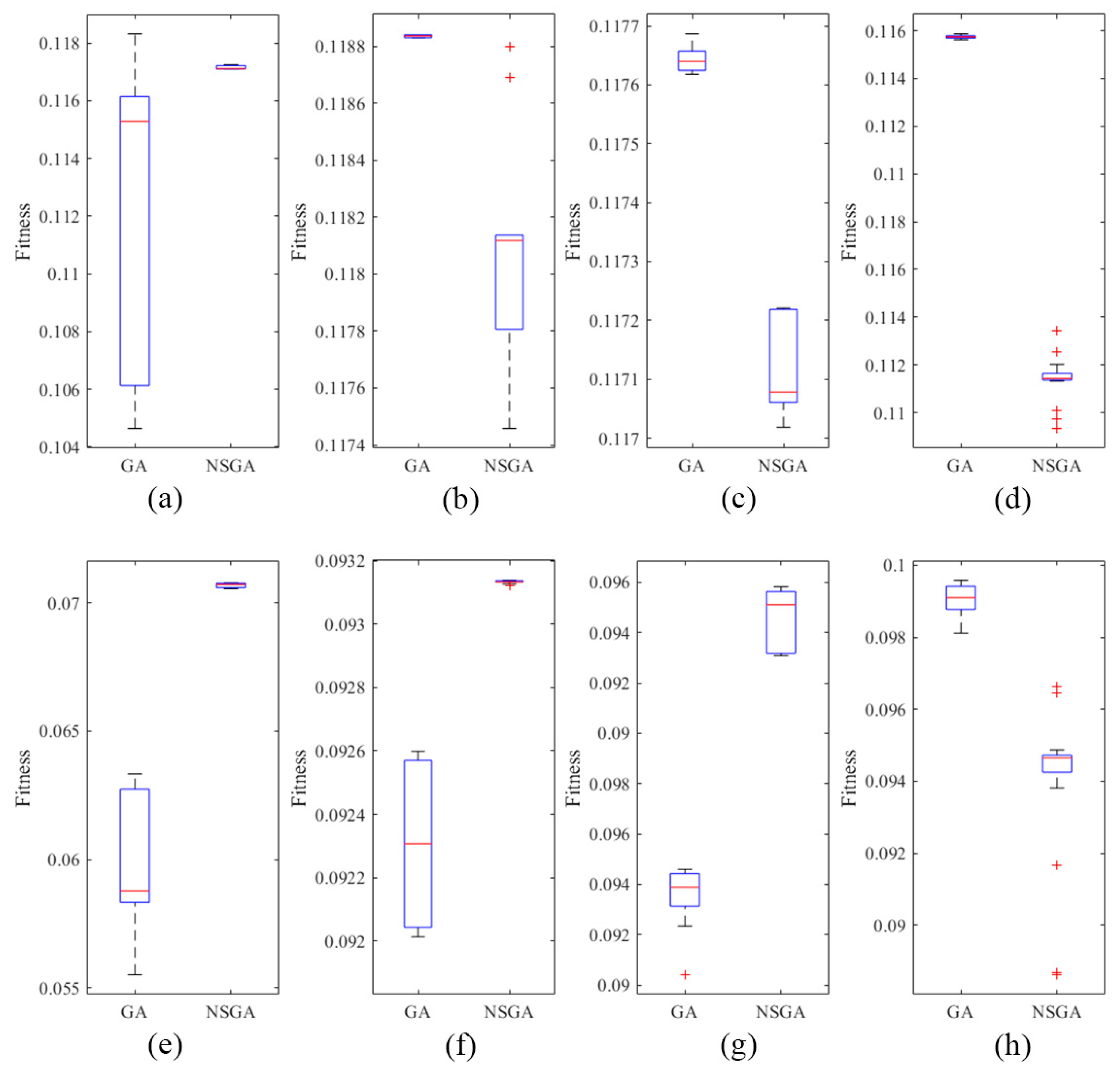
The performance of the solutions from our GA and NSGA was assessed using boxplot behavior analysis, the Wilcoxon rank-sum test, and performance metrics, as depicted in Figure 2,

Table 1. Statistical results of algorithms on two functions using Wilcoxon rank-sum test in the sugar example.

Objective Function	n = 7	n = 8	n = 9	n = 10
D-efficiency	0.1133	5.16 × 10−4	4.20 × 10−9	7.53 × 10−15
Min D-efficiency due to missing observation	0.0028	5.16 × 10−4	4.20 × 10−9	7.51 × 10−15

and

Table 2. The value of performance metrics in the sugar example.

Index	n = 7		n = 8		n = 9		n = 10
	GA	NSGA	GA	NSGA	GA	NSGA	GA	NSGA
HV	0.8715	0.8505	0.8343	0.8345	0.8364	0.8325	0.8309	0.8432
Spacing	1.02 × 10−4	1.26 × 10−4	4.45 × 10−7	9.29 × 10−5	1.46 × 10−4	4.17 × 10−5	2.49 × 10−5	6.33 × 10−5

, respectively. In the boxplot analysis shown in Figure 2b–d,g, the data spread for GA was noticeably narrower than for NSGA. This observation suggested that GA outperformed NSGA in terms of data distribution for D-efficiency when $n$ = 8 to 10, and in terms of minimum D-efficiency due to missing observations for $n$ = 9. For n = 10, GA and NSGA exhibited similar performances in terms of minimum D-efficiency resulting from missing observations, as illustrated in Figure 2h. Based on the Wilcoxon rank-sum test, as detailed in Table 1, the results indicated that (1) there was no difference in D-efficiency between GA7 and NSGA7; however, there was a difference in minimum D-efficiency due to missing observation between GA7 and NSGA7, (2) there is a difference in D-efficiency between GA and NSGA for $n$ = 8 to 10, and (3) there was a difference in minimum D-efficiency due to missing observations between GA and NSGA for $n$ = 10. For $n$ = 8 to 9, the D-efficiency of GA outperformed that of NSGA. For $n$ = 10, the minimum D-efficiency of GA due to missing observations was superior to that of NSGA. These outcomes aligned with the observations from Figure 2. Based on the quantitative performance metrics that were outlined in Table 2, our GA had exhibited the highest HV value for $n$ = 7 and 9. However, for $n$ = 8, the HV values of both GA and NSGA had been comparable. In terms of spacing values, GA’s values had generally been lower than those of NSGA, with the exception of $n$ = 9. Based on our analysis, we could infer that our GA had been comparable to NSGA-II in terms of convergence accuracy and statistical significance for most benchmark functions.

Figure 3, Figure 4, Figure 5 and Figure 6 display the distribution point patterns of all GA designs, all NSGA designs and the DX design for a range of design points from 7 to 10, respectively. Figure 7 illustrates the FDS plot for all GA designs, all NSGA designs and the DX design in the context of a complete design, whereas Figure 8 showcases the FDS plot for all GA designs, all GA designs and the DX design when the most impactful observation point was omitted.

Table 3. The D-, A-, G-, and IV-efficiency and the maximum loss of D, A, G, and IV-efficiency due to single missing observation in the sugar example.

$\mathit{n}$	Design	D-eff	A-eff	G-eff	IV-eff	$\mathbf{max} {\mathit{l}}_{\mathit{D}}$	$\mathbf{max} {\mathit{l}}_{\mathit{A}}$	$\mathbf{max} {\mathit{l}}_{\mathit{G}}$	$\mathbf{max} {\mathit{l}}_{\mathit{I}\mathit{V}}$
7	GA7.1	0.1046	2.8844 × 10−4	45.4001	0.1980	0.3946	0.8693	0.9753	0.8941
	GA7.2	0.1064	2.8896 × 10−4	49.9959	0.2033	0.4119	0.8661	0.9796	0.9055
	GA7.3	0.1129	2.9015 × 10−4	60.9705	0.2195	0.4696	0.8571	0.9882	0.9368
	GA7.4	0.1183	2.9248 × 10−4	68.7810	0.2301	0.5307	0.8388	0.9938	0.9633
	NSGA7.1	0.1171	2.7544 × 10−4	61.8542	0.2218	0.3961	0.8906	0.9683	0.8197
	DX7	0.1183	2.9272 × 10−4	68.9232	0.2299	0.5423	0.8363	0.9947	0.9682
8	GA8.1	0.1188	3.8096 × 10−4	83.3905	0.2419	0.2206	0.4536	0.8850	0.4198
	GA8.2	0.1188	3.8102 × 10−4	83.3579	0.2419	0.2210	0.4539	0.8854	0.4210
	GA8.3	0.1188	3.8130 × 10−4	83.0683	0.2418	0.2252	0.4566	0.8890	0.4321
	GA8.4	0.1188	3.8132 × 10−4	83.0354	0.2418	0.2256	0.4569	0.8894	0.4333
	NSGA8.1	0.1175	3.8314 × 10−4	80.3985	0.2431	0.2070	0.4331	0.8719	0.3929
	NSGA8.2	0.1178	3.8249 × 10−4	80.2739	0.2428	0.2094	0.4433	0.8742	0.3923
	NSGA8.3	0.1181	3.8185 × 10−4	80.6440	0.2426	0.2115	0.4494	0.8764	0.3939
	NSGA8.4	0.1188	3.8029 × 10−4	83.7217	0.2419	0.2161	0.4483	0.8809	0.4087
	DX8	0.1188	3.8093 × 10−4	82.6746	0.2417	0.2310	0.4636	0.8939	0.4389
9	GA9.1	0.1176	3.5533 × 10−4	75.3398	0.2244	0.2153	0.4301	0.8705	0.3864
	GA9.2	0.1176	3.5525 × 10−4	75.2591	0.2244	0.2164	0.4325	0.8716	0.3889
	GA9.3	0.1176	3.5556 × 10−4	74.7365	0.2243	0.2237	0.4402	0.8785	0.4090
	GA9.4	0.1177	3.5575 × 10−4	74.0821	0.2240	0.2334	0.4471	0.8874	0.4367
	NSGA9.1	0.1170	3.6787 × 10−4	80.2516	0.2418	0.1633	0.2547	0.8096	0.2972
	NSGA9.2	0.1171	3.6741 × 10−4	80.1273	0.2420	0.1643	0.2554	0.8110	0.3009
	NSGA9.3	0.1172	3.7130 × 10−4	79.0121	0.2427	0.1744	0.2483	0.8242	0.3273
	NSGA9.4	0.1172	3.7068 × 10−4	78.8122	0.2432	0.1763	0.2483	0.8266	0.3335
	DX9	0.1176	3.5303 × 10−4	73.7343	0.2237	0.2389	0.4592	0.8922	0.4496
10	GA10.1	0.1178	3.2133 × 10−4	74.4264	0.2105	0.1547	0.2762	0.7846	0.4118
	GA10.2	0.1178	3.2122 × 10−4	74.3539	0.2106	0.1553	0.2751	0.7855	0.4125
	GA10.3	0.1179	3.2750 × 10−4	73.4573	0.2114	0.1626	0.2799	0.7964	0.4049
	GA10.4	0.1179	3.3102 × 10−4	72.8185	0.2119	0.1682	0.2823	0.8044	0.4006
	NSGA10.1	0.1097	3.3079 × 10−4	63.3269	0.2110	0.1189	0.3415	0.6883	0.3935
	NSGA10.2	0.1107	3.4331 × 10−4	63.1228	0.2175	0.1442	0.2962	0.7486	0.3405
	NSGA10.3	0.1108	3.3626 × 10−4	62.7362	0.2168	0.1496	0.3020	0.7582	0.3411
	NSGA10.4	0.1117	3.3624 × 10−4	55.2538	0.2065	0.2068	0.4084	0.8445	0.3840
	DX10	0.1177	3.3199 × 10−4	69.8465	0.2115	0.1984	0.3021	0.8434	0.3955

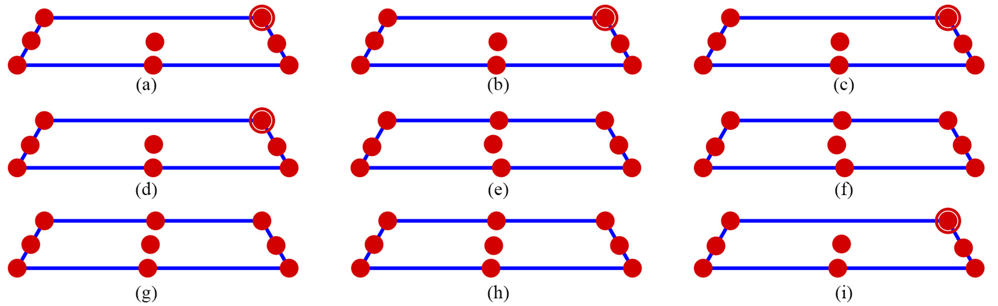
shows the D, A, G, and IV-efficiency and the maximum loss of D, A, G, and IV-efficiency due to a single missing observation. In Figure 3, for $n$ = 7, the distribution point patterns of all GA, NSGA and DX designs tended to occupy all vertices or locations near them, as well as positions close to two edge centroid points and near the overall centroid. The distribution point patterns of GA7.1, GA7.2, and GA7.3 designs were distinct, and they differed from those of the GA7.4 and DX7 designs. The GA7.4 and DX7 designs exhibited slight differences on the edge centroid points and overall centroid point, with other points being similar. In contrast, both the GA7.4 and DX7 designs varied from the NSAG7.1 design, particularly where their edge centroid points were located on different sides. Consequently, GA7.4 and DX7 designs demonstrated comparable performance in terms of D, A, G, and IV-efficiency as well as the maximum loss of D, A, G, and IV-efficiency due to a single missing observation. However, both GA7.4 and DX7 designs surpassed NSAG7.1 in measures of D, A, G, and IV-efficiency, and especially in the maximum loss of A-efficiency due to a single missing observation, as detailed in Table 1. Additionally, both GA7.4 and DX7 designs had identical FDS curves for the complete design and demonstrated better performance in terms of prediction variance, as shown in Figure 7a. However, when considering the FDS plot that omits the most impactful observation point, as illustrated in Figure 8a, the FDS curves of NSGA7.1 design appeared lower and flatter compared to the other designs. Meanwhile, the FDS curves of GA7.4 and DX7 designs were comparable, except at the boundary of the design region. As depicted in Figure 4, for $n$ = 8, the distribution point patterns of all GA, all NSGA and DX designs bore resemblance to those of $n$ = 7, but they tend to be closer to three edge centroid points, rather than two. In the case of $n$ = 9, as depicted in Figure 5, the point distribution patterns of all GA, NSGA, and DX designs resembled those of $n$ = 8. However, there was an additional replicated point at a vertex for both GA and DX designs, while the NSGA designs featured a point on the long edge centroid. Lastly, for $n$ = 10, the distribution point patterns of all GA and DX designs, as displayed in Figure 6, mirrored those for $n$ = 9, but with an added replicated point at two vertices. In contrast, the NSGA10 designs included an additional replicated point at one vertex, setting them apart from the GA10 and DX10 designs. Moreover, they did not mirror the patterns observed for $n$ = 9.

As a result, the GA and DX design demonstrate similar performance in terms of (1) D-, A-, G-, and IV-efficiency, and (2) the FDS curves for both the complete design and scenarios where the most impactful observation point is omitted, as indicated in Table 3 and Figure 7 and Figure 8. Based on D-efficiency, the GA and DX designs surpassed the NSAG designs. For A-efficiency, the GA, NSGA, and DX designs were comparable to each other. With respect to G-efficiency, the GA and DX designs were superior to the NSAG designs, except for $n$ = 9. However, in terms of IV-efficiency, the three designs—GA, NSGA, and DX—were closely matched, with the exception of $n$ = 9. Notably, most NSAG designs surpassed the GA and DX designs when considering the maximum efficiency loss due to a single missing observation. However, most GA designs outperformed the DX design when considering the maximum loss of D-, A-, G-, and IV-efficiency due to a single missing observation. As indicated in Table 3, the GA7.4 design neither possessed the highest D-, A-, G-, and IV-efficiency nor did it have the lowest maximum loss of D-, A-, G-, and IV-efficiency due to a single missing observation. Instead, it maintained a middle level for all these values, which was considered desirable. As demonstrated in Figure 7a and Figure 8a, the GA7.4 design, when compared to other GA7 designs, displayed robustness against missing observations in terms of prediction variance. On the other hand, the NSGA7.1 design emerged as the most robust against missing observations with respect to prediction variance. This distinction for the NSGA7.1 design was particularly evident in its FDS curves. They were notably flatter and lower in both the complete design and scenarios involving the omission of more impactful observations. For $n$ = 8, the FDS curves, depicted in Figure 7b and Figure 8b, revealed similar trends across all evaluated designs, whether considering the complete design or those scenarios that excluded key observations. For $n$ = 9, as showcased in Figure 7c and Figure 8c, the GA and DX designs maintained similar levels of robustness against missing observations for prediction variance. However, the NSGA designs demonstrated greater robustness in this aspect than the GA designs. Regarding n = 10, the FDS curves of all designs, with the exception of the NSGA10.4, were consistent when viewing the complete design and the scenarios that omitted significant observations, as seen in Figure 7d and Figure 8d. Nevertheless, when influential observations were excluded, the FDS curves for DX10 and NSGA10.4 became less competitive at the boundary of the design region, as indicated in Figure 8d.

From our analysis, it became evident that the designs generated by our Genetic Algorithm (GA) seemed to exhibit robust properties against missing observation in terms of prediction variance. Our algorithm focused on creating robust designs that performed well not only in terms of D-efficiency but also in terms of minimum D-efficiency due to missing observation. Our GA designs successfully achieved these objectives. Furthermore, they also provided commendable A-, G-, and IV-efficiency, as well as manageable maximum losses of A-, G-, and IV-efficiency due to a single missing observation.

Following the strong performance of our GA in generating optimal mixture designs, we provided four GA designs as a reference to help experimenters understand their performance and balance requirements. This assisted in assessing how well these designs aligned with user priorities and their robustness in handling missing observation. An assessment was performed using the desirability function based on the geometric mean, $D{F}_{Geo}$. Figure 9 showed the desirability function based on the geometric mean. The numbers displayed in Figure 8 corresponded to the numbers following the dots in the GA designs. The GA$n$.1 design was the optimal choice when the weight was 0, indicating that it was the optimal design based on the minimum D-efficiency due to missing observation. Conversely, the GA$n$.4 design was the optimal choice when the weight was 1, indicating that it was the optimal design based on the D-efficiency. The GA$n$.2 and GA$n$.3 designs became optimal when the weight ranged from 0.1 to 0.9, representing a trade-off between the minimum D-efficiency due to the missing observations and the D-efficiency. As illustrated in Figure 9, for $n$ = 7 and 9, the GA$n$.2 design was the optimal choice when the weight fell between 0.1 and 0.2. However, the GA$n$.3 design became the optimal choice when the weight was in the range of 0.3 to 0.9. For $n$ = 8, the GA8.2 design was optimal when the weight ranged from 0.1 to 0.5, and the GA8.3 design was optimal when the weight ranged from 0.6 to 0.9. Interestingly, for $n$ = 9, the GA9.2 design was the optimal choice when the weight was between 0.1 and 0.3, while the GA9.3 design became optimal for weights from 0.4 to 0.9. The $D{F}_{Geo}$ can serve as a tool, enabling experimenters to select the most robust optimal design based on their individual priorities. Therefore, in practice, if the primary focus of the experimenter was on minimizing the D-efficiency loss due to missing observations, the GA$n$.1 design would be preferred. However, if the emphasis was on the D-efficiency, the GA$n$.4 design would be more suitable. In cases where the experimenter wished to balance both criteria, the GA$n$.2 and GA$n$.3 designs would be the preferred choices.

6.2. Example 2: Mixture Problem as Presented in Myers et al. [2]

For our second example, we considered a mixture problem as presented by Myers et al. [2]. The lower and upper proportion constraints for this problem are as follows:

$$0.10\le x_1\le 0.80; 0.00\le x_2\le 0.75; 0.00\le x_3\le 0.60.$$

The boundary in this case consists of six vertices. Even though this example has the same number of components as the first example, the shape of the experimental region differs. Similar to the first example, we thoroughly examined the selection of GA parameter values before implementing the GA. We determined an appropriate number of generations for convergence, setting a limit of 1500 generations. Consequently, the genetic parameter values in this example differ from those in the first example. Furthermore, we established the following ranges for the genetic parameter values:

$$0.03\le {\alpha }_b\le 0.20, 0.03\le {\alpha }_{cb}, {\alpha }_{cw}\le 0.20, 0.005\le {\alpha }_e\le 0.15, 0.005\le {\alpha }_{mu}\le 0.10, 0.01\le \sigma \le 0.10.$$

Initially, the genetic parameter values are set to their maximum levels, and then systematically decreased to lower levels after 500 generations. In this example, the performance of the competing designs, encompassing 7 to 10 runs, is demonstrated. Figure 10 features the Pareto front, emphasized in gray, and illustrates a well-distributed set of optimal GA and optimal NSGA designs. These designs resulted from the application of a thinning technique to a rich Pareto front using $\epsilon$-dominance. The five GA designs chosen from the Pareto front, namely GAM$n$.1, GAM$n$.2, GAM$n$.3, GAM$n$.4, and GAM$n$.5, are denoted by red, blue, black, magenta, and cyan dots, respectively. The three NSGA designs chosen from the Pareto front, namely NSGAM$n$.1, NSGAM$n$.2, and NSGAM$n$.3, are denoted by red, magenta, and cyan dots, respectively.

As evidenced in the initial example, the gap between the highest and lowest D-efficiency, as well as the gap between the highest and lowest minimum D-efficiency due to a missing observation, were greater for $n$ = 7 compared to $n$ = 8 to 10 in the GA. Conversely, these gaps were generally smaller for NSGA than for GA, except in the cases of $n$ = 9. Moreover, the distribution patterns of the Pareto front for GA and NSGA exhibited distinct differences, as illustrated in Figure 10. The performance of the solutions from our GA and NSGA was assessed using boxplot behavior analysis, the Wilcoxon rank-sum test, and performance metrics, as depicted in Figure 11,

Table 4. Statistical results of algorithms on two functions using Wilcoxon rank-sum test in the Myers et al. [2] example.

Objective Function	n = 7	n = 8	n = 9	n = 10
D-efficiency	5.83 × 10−8	0.3257	2.81 × 10−11	2.27 × 10−4
Min D-efficiency Due to missing observation	5.38 × 10−8	0.4663	0.1855	2.27 × 10−4

and

Table 5. The value of performance metrics in the Myers et al. [2] example.

Index	n = 7		n = 8		n = 9		n = 10
	GA	NSGA	GA	NSGA	GA	NSGA	GA	NSGA
HV	0.3456	0.2393	0.2268	0.2245	0.2246	0.2276	0.2157	0.2111
Spacing	0.0050	0.0042	3.83 × 10−5	0.0058	6.37 × 10−5	0.0069	6.38 × 10−5	4.26 × 10−5

, respectively. In the boxplot analysis presented in Figure 11, the data spread for GA was notably wider than that for NSGA, although the range of the y-axis was quite small. Upon considering the Wilcoxon rank-sum test presented in Table 4, the results indicated that (1) there was no significant difference in D-efficiency and minimum D-efficiency due to missing observations between GA8 and NSGA8, (2) there was no significant difference in minimum D-efficiency due to missing observations between GA9 and NSGA9, (3) there was a significant difference in D-efficiency and minimum D-efficiency due to missing observations between GA and NSGA for n = 7 and 10, and (4) there was a notable difference in D-efficiency between GA9 and NSGA9. These results are consistent with the findings from the boxplot analysis. Based on the quantitative performance metrics presented in Table 5, our GA demonstrated superior performance by achieving the highest HV value and lower or comparable spacing across all design points. From this analysis, we can infer that our GA generally outperforms or is at least comparable to the NSGA-II in terms of convergence accuracy and statistical significance for the majority of benchmark functions.

As depicted in Figure 12, for $n$ = 7, the distribution point patterns of all GA and DX designs tended to be positioned on or near all vertices, as well as close to the overall centroid. In contrast, the distribution patterns of all points in NSGA7 were primarily near the overall centroid but did not necessarily align with or near all vertices. In the case of $n$ = 8, illustrated in Figure 13, the distribution point patterns of all GA and DX designs resembled those of $n$ = 7, but with an additional point near the edge centroid. The distribution patterns of all points in NSGA8 resembled those of the GA and DX designs. For $n$ = 9, as shown in Figure 14, the distribution point patterns of all GA and DX designs mirrored those of $n$ = 8, but they were located near two edge centroid points instead of one. On the other hand, the distribution patterns of all points in NSGA9 differed from those of NSGA8, including a point on the face and an edge centroid on the opposite side. Finally, when $n$ = 10, as depicted in Figure 15, the distribution point patterns of the GA and DX designs differed. However, the distribution patterns of the points for GA and NSGA designs exhibited similarities. The GA and NSGA designs tended to be located on or near all vertices, close to three edge centroid points and the overall centroid point. On the other hand, the DX designs were positioned on or near all vertices, at two replicated vertices, near an edge centroid point and the overall centroid point.

Figure 16 presents the FDS plot for all GA designs, all NSGA designs and the DX design for a complete design, while Figure 17 depicts the FDS plot for all GA designs, all NSGA designs and the DX design when the most impactful observation point is omitted.

Table 6. The D, A, G, and IV-efficiency and the maximum loss of D, A, G, and IV-efficiency due to single missing observation in the Myers et al. [2] example.

$\mathit{n}$	Design	D-eff	A-eff	G-eff	IV-eff	$\mathbf{max} {\mathit{l}}_{\mathit{D}}$	$\mathbf{max} {\mathit{l}}_{\mathit{A}}$	$\mathbf{max} {\mathit{l}}_{\mathit{G}}$	$\mathbf{max} {\mathit{l}}_{\mathit{I}\mathit{V}}$
7	GAM7.1	1.4533	0.1937	59.0077	0.2012	0.2989	0.9025	0.9177	0.9023
	GAM7.2	1.5341	0.2157	71.8442	0.2038	0.3713	0.9494	0.9651	0.9505
	GAM7.3	1.5470	0.2166	71.0432	0.1995	0.4416	0.9751	0.9829	0.9757
	GAM7.4	1.5470	0.2166	71.0432	0.1995	0.4416	0.9751	0.9829	0.9757
	GAM7.5	1.5576	0.2148	73.2303	0.1983	0.6120	0.9972	0.9982	0.9972
	NSGAM7.1	1.5093	0.2039	75.0825	0.2188	0.2294	0.8450	0.8793	0.8267
	NSGAM7.2	1.5231	0.2050	76.7376	0.2171	0.2463	0.8648	0.8980	0.8522
	NSGAM7.3	1.5258	0.2060	79.8187	0.2159	0.2579	0.8762	0.9111	0.8638
	DXM7	1.5628	0.2149	72.2797	0.1973	0.9957	1.0000	0.8516	1.0000
8	GAM8.1	1.5470	0.2166	71.0432	0.1995	0.4416	0.9751	0.9829	0.9757
	GAM8.2	1.5470	0.2166	71.0432	0.1995	0.4416	0.9751	0.9829	0.9757
	GAM8.3	1.5592	0.2054	83.6974	0.2092	0.2164	0.7588	0.8812	0.7452
	GAM8.4	1.5602	0.2045	83.4824	0.2074	0.2193	0.7634	0.8839	0.7545
	GAM8.5	1.5609	0.2053	83.4081	0.2086	0.2203	0.7645	0.8848	0.7543
	NSGAM8.1	1.5576	0.2054	83.9439	0.2111	0.2131	0.7544	0.8782	0.7386
	NSGAM8.2	1.5606	0.2051	83.4918	0.2075	0.2192	0.7640	0.8838	0.7490
	DXM8	1.5607	0.2049	83.4166	0.2081	0.2202	0.7647	0.8847	0.7509
9	GAM9.1	1.5256	0.2034	79.3612	0.2173	0.1525	0.5556	0.7886	0.5307
	GAM9.2	1.5325	0.2021	80.6834	0.2167	0.1596	0.5680	0.8046	0.5444
	GAM9.3	1.5413	0.2007	79.8332	0.2135	0.1669	0.5811	0.8145	0.5651
	GAM9.4	1.5423	0.2016	79.6607	0.2128	0.1684	0.5831	0.8165	0.5640
	GAM9.5	1.5448	0.2039	79.1202	0.2147	0.1734	0.5878	0.8229	0.5658
	NSGAM9.1	1.4993	0.2150	81.2746	0.2263	0.1393	0.2831	0.7685	0.3179
	NSGAM9.2	1.5020	0.2133	82.6615	0.2244	0.1444	0.2785	0.7823	0.2974
	NSGAM9.3	1.5117	0.2246	80.2923	0.2328	0.1629	0.3161	0.8091	0.2789
	DXM9	1.5461	0.2027	78.7305	0.2159	0.1770	0.5887	0.8276	0.5639
10	GAM10.1	1.5108	0.1953	85.6790	0.2195	0.0910	0.4790	0.6670	0.4488
	GAM10.2	1.5109	0.1956	85.6238	0.2191	0.0913	0.4797	0.6675	0.4525
	GAM10.3	1.5112	0.1960	85.2596	0.2192	0.0928	0.4789	0.6708	0.4509
	GAM10.4	1.5114	0.1963	85.0476	0.2194	0.0937	0.4783	0.6728	0.4541
	GAM10.5	1.5116	0.1966	84.7067	0.2189	0.0952	0.4779	0.6759	0.4502
	NSGAM10.1	1.5285	0.1932	88.6606	0.2191	0.0795	0.4982	0.6408	0.4689
	NSGAM10.2	1.5285	0.1932	88.6165	0.2186	0.0797	0.4983	0.6412	0.4734
	DXM10	1.5446	0.1801	69.5099	0.1828	0.2017	0.7879	0.8471	0.7734

shows the D, A, G, and IV-efficiency as well as the maximum loss of D-, A-, G-, and IV-efficiency due to a single missing observation. The GA design and DX design exhibited comparable performance in terms of prediction variance, with the exception of the GAM7.1 design, which showed inferior performance at the boundary, as illustrated in Figure 16a and Figure 17a. Both the GAM7.2 and GMM7.3 designs demonstrated similar FDS curves in the complete design and when the most impactful observation point was omitted. Consequently, these designs appeared to possess robust properties against missing observations. The NSGAM7 designs, however, did not appear to have such robust properties against missing observations, as illustrated in Figure 16a and Figure 17a. The GAM7 and DXM7 designs were largely equivalent in terms of D-, A-, G-, and IV-efficiency, but the DXM7 design fell short when considering the maximum loss of D-, A-, G-, and IV-efficiency due to a single missing observation, as detailed in Table 6. Nonetheless, the NSGA7 designs demonstrated good performance in terms of the maximum loss of efficiency due to a single missing observation. For $n$ = 8 and 9, the FDS curves for the complete design of the NSGA designs were lower than those of the GA and DX designs, though they were comparable at the design space boundary.

The FDS curves displayed notable similarity across all competing designs when the most impactful observation point was omitted. As a result, the GA, NSGA and DX designs seemed to exhibit robust properties in the face of missing observation. The GAM8.3, GAM8.4, GAM8.5, NSGAM8.1, NSGAM8.2 and DXM8 designs were quite comparable in terms of D-, A-, G-, and IV-efficiency, as well as the maximum loss of D, A, G, and IV-efficiency due to a single missing observation. Meanwhile, for $n$ = 9, the GAM9 and DXM9 designs showed a similar comparison in terms of D-, A-, G-, and IV-efficiency, and also in the maximum loss of these efficiencies due to a single missing observation. However, the NSGA9 designs did not perform well in terms of D-efficiency. For $n$ = 10, as illustrated in Figure 16d and Figure 17d, the FDS curves of the GA and NSGA designs outperformed the DX design for both the complete design and when the most impactful observation point was omitted. The FDS curves of the GA and NSGA designs were identical in both the complete design and when the most impactful observation point was omitted. The GAM10 and NSGAM10 designs outperformed in terms of D-, A-, G-, and IV-efficiency, and also showed a smaller maximum loss of these efficiencies due to a single missing observation. Consequently, the GAM10 and NSGAM10 designs appeared to possess strong robustness properties when faced with missing observations. These observations emphasize that even though designs may appear comparable based on prediction variance, it does not necessarily imply comparability on other criteria. When comparing the robustness of designs due to missing observation, experimenters should consider multiple criteria. Based on these results, we can conclude that our GA exhibited the ability to generate an optimal mixture design despite missing observations.

Upon demonstrating the effectiveness of our GA in creating optimal mixture designs, we made available four reference GA designs. This allowed experimenters to assess their performance and effectively balance their requirements. Figure 18 displays the desirability function based on the geometric mean, which helps assess how well these designs align with user priorities and their robustness in handling missing observations. The GAM$n$.1 design emerged as the optimal choice when the weight was 0, indicating its optimal performance based on the minimum D-efficiency due to missing observation. Conversely, the GAM$n$.5 design was the optimal choice when the weight was 1, signifying its superiority based on D-efficiency. The GAM7.2 design became optimal for weights ranging from 0.1 to 0.6, whereas the GAM7.3 design took precedence for weights between 0.7 and 0.9. The GAM8.2 design was optimal for weights ranging from 0.1 to 0.8, while the GAM8.3 design stood out when the weight was 0.9. For $n$ = 9, the GAM9.2 design was the optimal choice for weights between 0.1 and 0.3. The GAM9.3 design became optimal for weights between 0.4 and 0.7, and the GAM9.4 design excelled for weights between 0.8 and 0.9. Finally, for $n$ = 10, the GAM10.2 design was optimal for weights between 0.1 and 0.3. The GAM10.3 design took the lead for weights between 0.4 and 0.5, and the GAM10.4 design was optimal for weights ranging from 0.6 to 0.9. In practice, if an experimenter aims to balance both the D-efficiency and the minimum D-efficiency loss due to missing observations, the GA designs optimal for each weight may serve as good choices. This is because they can facilitate trade-offs between the two criteria and demonstrate robustness against missing observations. Their performance is measured based on prediction variance, optimality criteria, and loss of efficiency.

7. Conclusions

In real-world situations, even well-planned experiments can encounter missing observations. When repeating experiments to account for missing observations is infeasible, experimenters often favor more robust designs to protect against potential information loss. This paper introduces a multi-objective genetic algorithm to create optimal mixture designs resilient to missing observations, focusing on cases with three mixture components and irregularly shaped experimental regions. Our genetic algorithm balances D-efficiency and minimal D-efficiency loss due to missing observations when solving multi-objective optimization problems. The emphasis on D-efficiency is due to several reasons: (1) if any observation is missed from a D-optimal design, the overall impact on the accuracy of the parameter estimates can be minimized; (2) the loss of some observations does not disproportionately affect specific regions of the experimental space, thereby ensuring the reliability of the experimental results even when data is missing; and (3) a D-optimal design ensures that the remaining data are as informative as possible, maximizing the utility of the available data. As for the distributional patterns of the GA designs, most of the design points are located at or close to the vertices, near the edge centroid points, and near the overall centroid point. In scenarios where the experimental region has six vertices corresponding to the number of parameters, missing observations at the near overall centroid point or the most impactful point can lead to insufficient information for accurately estimating all the model parameters using some optimal designs. Our findings align with Rashid et al. [46], confirming that missing the near overall centroid point, which significantly impacts D-efficiency, greatly affects the accuracy of model parameter estimates. From the results, it is clear that (1) our algorithm can generate optimal mixture designs that perform well in both D-efficiency and the mitigated loss of D-efficiency, and (2) our algorithm can produce optimal mixture designs that demonstrate substantial robustness against missing observations. This robustness is substantiated by three key factors: (1) predictive variance, (2) D, A, G, and IV-efficiency, and (3) the loss of efficiency with respect to D-, A-, G-, and IV-efficiency. Furthermore, our GA design continues to perform well in terms of A-, G-, and IV-efficiency, and in minimizing the loss of efficiency based on these criteria. In fact, the GA designs perform as well as, if not better than, the NSGA and DX designs when considering these three key factors. Experimenters can select the optimal design for each weight using the desirability function from this comprehensive set of mixture designs. They can then choose a design that strikes an ideal balance between objective functions according to their priorities. Our method is flexible and can be easily adapted to other scenarios, such as when multiple component constraints exist, the number of components exceeds three, or when considering other optimality criteria. We propose our genetic algorithm as a practical alternative for generating optimal mixture designs that are robust due to missing experimental observation. Our findings suggest that experimenters can have confidence in the proposed GA designs, as they perform comparably to, if not better than, the designs generated using another method in terms of robustness against missing observations. However, if protection against the worst-case scenario for parameter estimation is a priority, we recommend the proposed GA designs. Moreover, when the experiment is subject to resource constraints and missing observations are a frequent concern, a design robust against missing observation should be given serious consideration.

The computing time required to construct optimal mixture designs can vary based on factors such as the number of chromosomes (population size) and the number of design points. In the examples presented in this paper, the time duration for generating GA designs ranges approximately from 25 to 40 min. In contrast, the design generation using the NSGA was slightly faster, taking an estimated 20 to 35 min. The number of chromosomes has a significant impact on the computing time, as larger populations require evaluating more potential solutions in each generation. In our research, we have utilized a population size of 100, which is consistent with the work by Deb et al. [27]. However, it is worth considering that reducing the population size in future studies may be a practical approach to decrease computing time. By doing so, the algorithm can potentially complete its computations faster. However, our algorithm has some limitations: the computational cost increases exponentially as the number of objective functions and the population size increases.

Potential future extensions of our algorithm include its application to the construction of optimal mixture-process experimental designs involving both control and noise variables. Such designs would be well-suited for use in mixture experiments within chemical and production industries. Furthermore, exploring the use of D-efficiency, minimum D-efficiency, and median D-efficiency as the multi-objective functions for the genetic algorithm could significantly enhance its versatility and applicability in various domains. Additionally, the use of other multi-objective heuristic algorithms to generate optimal exact mixture designs can be considered.