Controlled Arrivals on the Retrial Queueing–Inventory System with an Essential Interruption and Emergency Vacationing Server

Abstract

In recent times, we have encountered new situations that have imposed restrictions on our ability to visit public places. These changes have affected various aspects of our lives, including limited access to supermarkets, vegetable shops, and other essential establishments. As a response to these circumstances, we have developed a continuous review retrial queueing–inventory system featuring a single server and controlled customer arrivals. In our system, customers arriving to procure a single item follow a Markovian Arrival Process, while the service time for each customer is modeled by an exponential distribution. Inventories are replenished according to the $(s,Q)$ reordering policy with exponentially distributed lead times. The system controls arrival in the waiting space with setup time. The customers who arrive at a not allowed situation decide to enter an orbit of infinite size with predefined probability. Orbiting customers make retrials to claim a place in the waiting space, and their inter-retrial times are exponentially distributed. The server may experience essential interruption (emergency situation) which arrives according to Poisson process. Then, the server goes for an emergency vacation of a random time which is exponentially distributed. In the steady-state case, the joint probability of the number of customers in orbit and the inventory level has been found, and the Matrix Geometric Method has been used to find the steady-state probability vector. In numerical calculations, the convexity of the system and the impact of F-policy and emergency vacation in the system are discussed.

1. Introduction

Recently, social and physical isolation measures, including lockdowns of workplaces, schools, and general social life, which have become standard to curb the spread of disease, have disturbed many typical elements of life, including sports and physical exercise. The pandemic crisis is the reason for all of these things. We have been grappling with a bunch of problems since then, in addition to the ones listed above. The pandemic situation made dramatic changes to the environment, which also had a lot of impacts on the retail industry’s operations. The crisis has resulted in significant variations in company performance across many aspects of corporate action. As a result of travel restrictions, social distancing, restrictions on the sale of some commodities, and customers feeling compelled to resort to budget cuts and deferring projects, sales suffered a sharp decline. Because of the sudden drop in sales revenue, companies dealing with more commodities struggled to recover fixed expenditures. We refer readers to Anbazhagan [1], Jeganathan [2], and Samanta et al. [3] to learn more about inventory systems.

Many retailers dealing with the queueing–inventory system have faced questions like whether the arrival has to be controlled or the service has to be controlled in the shop at times like the above-mentioned pandemic scenario. In our proposed model, we considered the control upon the customer’s arrival, as first introduced by Gupta [4]. In that sense, the notion of an F-policy on queueing systems prohibits newly arriving customers from joining the system once it reaches its maximum capacity H until the capacity has diminished to the threshold value, say F$(0\le F\le H)$. After that, the server probably needs time to set up before customers use the system. Furthermore, this study investigates the inter-relationship between the problems of controlling arrivals and controlling services. Wang et al. [5] examine a supplementary variable technique and a recursive method for the queueing system with generally distributed arrivals, with an F-policy and an exponential startup time. Yang et al. [6] analyzed a queueing system with arrival control, startup time, and working vacation using the matrix analytic method. Then, they used the direct search method and the quasi-Newton method to determine the optimal values. The Bernoulli F-policy and F-policy have been investigated by Chang et al. [7,8], as well as by many researchers like Jain and Sanga [9] and Ke et al. [10] in the queueing system.

During customer service, the server needs some random time to rest or perform other work. That break time is said to be a server vacation. In the literature, many researchers are conducting their research on the topic of server vacations, and they also propose various types of vacations. We refer the reader to Jain et al. [11], Nithya et al. [12], Rani et al. [13] and Zhang [14] for various server vacations. Among those types of vacations, an emergency vacation plays an important role because, at any time of service, the server could confront some crucial or unexpected emergency situation that impedes them from continuing to serve the customers as usual and prompts the server to take an emergency vacation. Chandra Shekhar et al. [15] proposed the concept of emergency vacation for servers in queueing systems. The optimal control of the system has been found using metaheuristic and heuristic optimization techniques. We refer readers to Ayyappan et al. [16,17] and Vaishnawi et al. [18] for emergency vacation.

Every server has experienced interruptions during service time due to family, government, or other factors. These interruptions lead them to take vacations. The literature considers two types of interruptions: service interruptions and vacation interruptions. In analyzing an inventory system, Krishnamoorthy et al. [19] took service interruptions and retrials into account. Krishnamoorthy et al. [20] also investigated the interruption concept in the production inventory system, which has a service time. Fiems et al. [21] investigated different types of server interruptions in the queueing system. Therefore, interruptions can occur anytime during the service (or vacation). During those interruptions, the server may experience many unwanted or unimportant interruptions, which are not worth taking a vacation over compared to the pandemic, as mentioned earlier. So, the server takes a vacation only when the interruption is essential, taking such interruptions that lead the server to go on vacation as motivation to consider essential interruptions in this model. Most researchers have considered the concept of “interruption” as a breakdown. In Ke [22], Wu et al. [23], and Xu et al. [24], the authors have discussed the vacation policy and the breakdown repair separately. If the server breaks down during the service, it goes through the repair process. According to their model, the server takes a vacation when the system is empty or upon the completion of the repair process without the influence of breakdown. After the breakdown, the server has been repaired, and it goes to serve the customers immediately. However, in the case of vacation after the interruption, the server has time to self-recover and ensure the clearance of the interruptions. The vacation duration may lead the customer to become impatient or lost. Moreover, for more details about the retrial and impatience of the customer, we refer to Anbazhagan [25,26] and Melikov and Shahmaliyev [27] for retrial concepts and to Al Hamadi et al. [28] for the impatience of the customers in the system.

This paper considers a single server retrial queueing–inventory system in which customers arrive according to a Markovian Arrival Process (MAP), also known as the versatile point process. By choosing the parameters of the MAP appropriately, the underlying arrival process can be made as a renewal process. Therefore, the MAP is a tractable class of Markovian renewal processes. The MAP is a rich class of Poisson processes that includes well-known processes such as the Poisson, PH-renewal, and Markov-modulated Poisson processes. As is well known, Poisson processes are simple and tractable ones used widely in stochastic modeling. The idea of the MAP is to generalize the Poisson process significantly while still keeping its tractability.

In many practical applications, the arrival does not follow a renewal process. So, the MAP is the most convenient tool to model renewal and non-renewal appearance cases. In this model, the MAP allows us to have realistic arrival patterns, capturing dependencies and correlations between arrivals. Furthermore, the MAP is defined for discrete and continuous times, but we need the continuous-time case. For more details about the MAP and its properties, see Chakravarthy [29] and Neuts [30].

A continuous-time MAP is based on the underlying Markov chain, which is irreducible and has a generator $P^{\ast }=\left(p_{ij}\right)$. The sojourn time in the state i follows an exponential distribution with parameter ${\lambda }_i=-p_{ii}$, and then it stays in state i. There is a possibility of the occurrence of two events: $\left(1\right)$ with probability $q_{ij}\left(1\right)$, the Markov chain transitions to j with an arrival; $\left(2\right)$ with probability $q_{ij}\left(0\right)$, the Markov chain transitions to j without an arrival. We define $D_0=\left(d_{ij}^0\right)$ and $D_1=\left(d_{ij}^1\right)$, which satisfy $d_{ii}^0={\lambda }_{ii};d_{ij}^0={\lambda }_i{q}_{ij}\left(0\right),i\ne j$ and $d_{ij}^1={\lambda }_i{q}_{ij}\left(1\right)$. Then, $P^{\ast }$ is given by $P^{\ast }=D_0+D_1$, where $D_0$ governs the transitions without an arrival and $D_1$ governs the transitions with an arrival.

1.1. Motivation

During the pandemic, we have seen and realized the problems of the servers in hospitals, grocery shops, medical shops, and all other essential buying stations. The server will not dump the waiting space with customers to ensure safety. To avoid this, the server uses a queueing term known as the F-policy, which stands for customer arrival control. That is, when the waiting area achieves its maximum amount of space, the server restricts customers from joining the system until it touches the threshold value F, which occurs after the customers have received service in the system. On or after the threshold value, if the server finds a new arrival to the waiting space, then the server needs to perform some setup work like sanitizing to allow that customer in after completing the ongoing service of the customer. The customers who arrive during the prohibition time may retry to claim a place in the waiting space after some time. During the customer’s service, the server may be interrupted essentially by the arrival of some emergency situations like personal problems or the things which cause problems. That interruption leads the server to go on a vacation, which we denote as an emergency vacation. Upon completion of service, the customers receive their demanded item. The server’s requirement to guarantee the clients’ safety during the pandemic and their experience with disruptions, which are the barriers to making a profit in their job, are the driving forces for this research.

1.2. Research Gap

According to the literature, the F-policy and emergency vacations have been widely employed solely in queueing systems through the concepts such as optional service, server failure, server vacations, vacation disruptions, and many others. To the best of our knowledge, no literature exists with controlled arrival on queueing inventory systems. To address this, we have modeled a retrial queueing–inventory system, including controlled arrival and emergency vacation led by the arrival of essential interruptions. In this model, we considered that the server takes a vacation on the influence of the arrival of an essential interruption. This model investigates when the server experiences all their struggles (such as controlled arrival, essential interruption, emergency vacation, and customer impatience) in a queueing–inventory system and how the server optimizes the system’s profit through sensitivity and cost analyses.

1.3. Contribution of the Model

The following presumptions are to be carried out in this paper:

• This model investigates the controlled arrival, essential interruption, and emergency vacation of a retrial queueing-inventory system.
• This model uses the matrix geometric method to determine the proposed system’s steady-state probability vector.
• The numerical illustration analyzed the system performance measures using parameter variation.
• The optimal cost of the model is obtained under parameter variation.

1.4. Layout of the Article

The article is laid out as follows: The constructed model is described in Section 2. In Section 3, the occurrences of transitions are explained in detail using the transition form and the transition matrix form. Section 4 describes the matrix’s geometric approximation to find the system’s stability condition and steady-state behavior. Section 5 and Section 6 examine the performance measures of the system and the numerical calculation, which has shown the convexity of the total cost, and present discussions about the sensitivity analysis of the model. The cost analysis of the above-considered model is studied in Section 7. Section 8 contains the conclusion and related future directions.

2. Model Description

This model considers a single-server retrial queueing–inventory system with a controlled arrival stream of customers to the system with server interruptions and emergency vacations. It has an infinite orbit and a finite waiting space $\left(H\right)$ attached to the server.

2.1. Arrival Process

Customers arrive according to the Markovian Arrival Process (MAP). The MAP has been determined using an irreducible Markov process $\{v_t,t\ge 0\}$ with the finite state space $\{1,2,\dots ,u\}$. W is the generator of the transition rates of the Markov process $v_t$, and it is described in additive form as $W=W_0+W_1$, where the sub-generator $W_0$ defines the transition rates of the underlying Markov process, which does not cause arrival. The non-negative matrix $W_1$ defines the transition rates of the Markov process, which are governed by the customer’s arrival.

Let $\pi$ be the invariant probability row vector of the Markov process with generator W, which can be obtained from the system of linear algebraic equations $\pi W=\mathbf{0},\pi \mathbf{e}=1$, as the unique solution. Furthermore, here, e denotes a column vector of 1s, and 0 denotes a row vector of 0s with appropriate dimension. Let $\zeta$ represent the starting probability vector of the underlying Markov chain governing the MAP. The stationary MAP is obtained by selecting $\zeta =\pi$ after that. In the stationary form of the MAP, the fundamental rate, or constant $\lambda =\pi W_1\mathbf{e}$, determines the anticipated number of arrivals per unit of time.

2.2. Controlled Arrival Process (F-Policy)

The arriving customers are allowed to enter the waiting space. Suppose the waiting space reaches its capacity H (i.e., the waiting space becomes full). In that case, the customers are prohibited (not allowed) from entering it according to the F-policy (arrival control policy) until enough customers already in the waiting space have been served with an exponentially distributed service rate alpha so that the number of customers in the waiting space descends to the threshold level $F(0<F<H)$.

Setup: Once the waiting space reaches the threshold level, the server prepares to allow customers inside by performing setup work upon the customer’s arrival. That means, upon service completion, if the server finds an arrival after reaching the threshold value, then the server needs to perform some setup work to allow the customers into the waiting space. The time taken for the setup work is distributed exponentially with a rate $\eta$. From that moment, the system behaves normally until the waiting space becomes full, at which time the entire process is repeated.

2.3. Retrial Process and Customer Impatience

A full waiting space or during the prohibition of entry into the waiting space, the arriving customers may enter the orbit with a probability p or exit with a probability $q(=1-p)$. They tried multiple times to obtain a place in the designated waiting space. The orbiting customers claim their place on successful retrial (when the waiting space is in an allowed state). Intervals between attempts have an exponential distribution with rate $g_1\theta$, where $g_1$ is the number of customers in orbit. This model follows classical retrial policy, i.e., customers in orbit act independently. The orbiting customers become impatient during retrials, which is distributed exponentially with the parameter $\gamma$ depending on the number of customers in the orbit.

2.4. Service Process

Customers from the waiting space receive their service with exponentially distributed service rate $\alpha$. Their service is completed with the receipt of the demanded item.

2.5. Replenishment

The service completion of the customer reduces one item from the inventory. Likewise, when the inventory level drops to the reorder level s, according to the $(s,Q)$ ordering policy, the server places an order for $Q(=S-s)>s$. If the server finds zero inventory in the system, it waits in that position until replenishment occurs. The replenishment rate is distributed exponentially with $\mu$.

2.6. Essential Interruption

During the customer’s service, the server may be interrupted by the occurrence of an essential interruption (emergency situation) under the Poisson process with rate $\beta$. This disrupts the service of the customer. The service-interrupted customer returns to the head of the waiting space and waits until they receive service.

2.7. Emergency Vacation

When the server becomes interrupted by the arrival of essential interruption, instantly, the server goes for a vacation of a random time, which is said to be an emergency vacation. The vacation time has an exponential distribution with rate $\kappa$. Upon completion of the vacation, the server continues to serve the customers who wait in the waiting space. If the waiting space is zero upon vacation completion, the server waits in the system until the customer’s arrival.

3. Transition Analysis

For modeling purposes, the states of the governing queueing–inventory system model at time instant ’t’ are specified as $G_1\left(t\right),G_2\left(t\right),G_3\left(t\right),G_4\left(t\right)$, and $G_5\left(t\right)$, which denote the number of customers in the orbit, the inventory level, the number of customers in the waiting space, the server status, and the phase of the arrival process, respectively. Then, the quintuplets

$$K=\{G_1\left(t\right),G_2\left(t\right),G_3\left(t\right),G_4\left(t\right),G_5\left(t\right);t\ge 0\}$$

where

$G_4\left(t\right)=\left\{\begin{array}{cc}1\hfill & \mathrm{Server}\mathrm{is}\mathrm{on}\mathrm{emergency}\mathrm{vacation}\mathrm{and}\mathrm{customers}\mathrm{are}\mathrm{not}\mathrm{allowed}\mathrm{to}\hfill \\ \hfill & \mathrm{enter}\mathrm{the}\mathrm{system}\hfill \\ 2\hfill & \mathrm{Server}\mathrm{is}\mathrm{busy}\mathrm{and}\mathrm{customers}\mathrm{are}\mathrm{not}\mathrm{allowed}\mathrm{to}\mathrm{enter}\mathrm{the}\mathrm{system}\hfill \\ 3\hfill & \mathrm{Server}\mathrm{is}\mathrm{busy}\mathrm{and}\mathrm{customers}\mathrm{are}\mathrm{allowed}\mathrm{to}\mathrm{enter}\mathrm{the}\mathrm{system}\hfill \\ 4\hfill & \mathrm{Server}\mathrm{is}\mathrm{on}\mathrm{an}\mathrm{emergency}\mathrm{vacation}\mathrm{and}\mathrm{customers}\mathrm{are}\mathrm{allowed}\mathrm{to}\hfill \\ \hfill & \mathrm{enter}\mathrm{the}\mathrm{system}\hfill \end{array}\right.$

is a stochastic process with state space

$$\begin{array}{ccc}\hfill \mathbb{G}& =& \{(g_1,g_2,g_3,g_4,g_5);g_1\ge 0;0\le g_2\le S;0\le g_3\le H;g_4=1,2;1\le g_5\le u\}\cup \hfill \\ \hfill & & \{(g_1,g_2,g_3,g_4,g_5);g_1\ge 0;0\le g_2\le S;0\le g_3\le H-1;g_4=3,4;1\le g_5\le u\}\hfill \end{array}$$

It can be shown that the stated stochastic process K of the queueing–inventory system with state space $\mathbb{G}$ is a Markov process based on the assumptions made on the input and output processes. Then, the infinitesimal generator of this process can be determined by the arguments given below.

3.1. Elucidation of Transitions

In this section, the occurrence of transitions are explained.

• Transitions due to the arrival of customers to the orbit.
  The arriving customers may choose to enter the orbit with probability p whenever the waiting space is prohibited upon their arrival.

  (a)

  $$\begin{gathered} (g_1,g_2,g_3,g_4,g_5)\underrightarrow{p{W}_1}(g_1+1,g_2,g_3,g_4,g_5); \\ {g}_1\ge 0;0\le g_2\le S;0\le g_3\le H;g_4=1,2;1\le g_5\le u \end{gathered}$$

• Transitions due to the customers’ arrival to the waiting space.
  Customers can arrive at the waiting space in two ways: one is customers directly enter the waiting space when the waiting space is in an allowed state; another one is customers from orbit enter via retrials.

  (a)

  $$\begin{gathered} (g_1,g_2,g_3,g_4,g_5)\underrightarrow{W_1}(g_1,g_2,g_3+1,g_4,g_5); \\ {g}_1\ge 0;0\le g_2\le S;0\le g_3\le H-2;g_4=3,4;1\le g_5\le u \end{gathered}$$

  (b)

  $$\begin{gathered} (g_1,g_2,H-1,3,g_5)\underrightarrow{W_1}(g_1,g_2,H,2,g_5); \\ {g}_1\ge 0;0\le g_2\le S;1\le g_5\le u \end{gathered}$$

  (c)

  $$\begin{gathered} (g_1,g_2,H-1,4,g_5)\underrightarrow{W_1}(g_1,g_2,H,1,g_5); \\ {g}_1\ge 0;0\le g_2\le S;1\le g_5\le u \end{gathered}$$

• Transitions due to the successful retrials:

  (a)

  $$\begin{gathered} (g_1,g_2,g_3,g_4,g_5)\underrightarrow{g_1\theta I_u}(g_1-1,g_2,g_3+1,g_4,g_5); \\ {g}_1\ge 1;0\le g_2\le S;0\le g_3\le H-2;g_4=3,4;1\le g_5\le u \end{gathered}$$

  (b)

  $$\begin{gathered} (g_1,g_2,H-1,3,g_5)\underrightarrow{g_1\theta I_u}(g_1-1,g_2,H,2,g_5); \\ {g}_1\ge 1;0\le g_2\le S;1\le g_5\le u \end{gathered}$$

  (c)

  $$\begin{gathered} (g_1,g_2,H-1,4,g_5)\underrightarrow{g_1\theta I_u}(g_1-1,g_2,H,1,g_5); \\ {g}_1\ge 1;0\le g_2\le S;1\le g_5\le u \end{gathered}$$

• Transitions due to the service completion.
  Customers from the waiting space complete their service by attaining one unit of an item, which makes the transitions take the following forms:

  (a)

  $$\begin{gathered} (g_1,g_2,g_3,g_4,g_5)\underrightarrow{\alpha I_u}(g_1,g_2-1,g_3-1,g_4,g_5); \\ {g}_1\ge 0;1\le g_2\le S;1\le g_3\le H-1;g_4=2,3;1\le g_5\le u \end{gathered}$$

  (b)

  $$\begin{gathered} (g_1,g_2,H,2,g_5)\underrightarrow{\alpha I_u}(g_1,g_2-1,H-1,2,g_5); \\ {g}_1\ge 0;1\le g_2\le S;1\le g_5\le u \end{gathered}$$

• Transitions due to replenishment of inventory.

  (a)

  $$\begin{gathered} (g_1,g_2,g_3,g_4,g_5)\underrightarrow{\mu I_u}(g_1,g_2+Q,g_3,g_4,g_5); \\ {g}_1\ge 0;0\le g_2\le s;0\le g_3\le H-1;1\le g_4\le 4;1\le g_5\le u \end{gathered}$$

  (b)

  $$\begin{gathered} (g_1,g_2,H,g_4,g_5)\underrightarrow{\mu I_u}(g_1,g_2+Q,H,g_4,g_5); \\ {g}_1\ge 0;0\le g_2\le s;g_4=1,2;1\le g_5\le u \end{gathered}$$

• Transitions due to the occurrence of essential interruptions.
  An essential interruption may occur at any time in between customer service.

  (a)

  $$\begin{gathered} (g_1,g_2,g_3,2,g_5)\underrightarrow{\beta I_u}(g_1,g_2,g_3,1,g_5); \\ {g}_1\ge 0;0\le g_2\le S;0\le g_3\le H;1\le g_5\le u \end{gathered}$$

  (b)

  $$\begin{gathered} (g_1,g_2,g_3,3,g_5)\underrightarrow{\beta I_u}(g_1,g_2,g_3,4,g_5); \\ {g}_1\ge 0;0\le g_2\le S;0\le g_3\le H-1;1\le g_5\le u \end{gathered}$$

• Transitions due to the essential interruption.
  The occurrence of essential interruption takes the server to an emergency vacation during the service.

  (a)

  $$\begin{gathered} (g_1,g_2,g_3,1,g_5)\underrightarrow{\kappa I_u}(g_1,g_2,g_3,2,g_5); \\ {g}_1\ge 0;0\le g_2\le S;0\le g_3\le H;1\le g_5\le u \end{gathered}$$

  (b)

  $$\begin{gathered} (g_1,g_2,g_3,4,g_5)\underrightarrow{\kappa I_u}(g_1,g_2,g_3,3,g_5); \\ {g}_1\ge 0;0\le g_2\le S;0\le g_3\le H-1;1\le g_5\le u \end{gathered}$$

• Transitions due to the setup time of the server.
  The server needs some setup time to allow the customers to enter the waiting space whenever the system reaches F after the service of the customers.

  (a)

  $$\begin{gathered} (g_1,g_2,g_3,1,g_5)\underrightarrow{\eta I_u}(g_1,g_2,g_3,4,g_5); \\ {g}_1\ge 0;0\le g_2\le S;0\le g_3\le F;1\le g_5\le u \end{gathered}$$

  (b)

  $$\begin{gathered} (g_1,g_2,g_3,2,g_5)\underrightarrow{\eta I_u}(g_1,g_2,g_3,3,g_5); \\ {g}_1\ge 0;0\le g_2\le S;0\le g_3\le F;1\le g_5\le u \end{gathered}$$

3.2. Construction of Block Matrix

The block-structured infinitesimal generator matrix of the continuous-time Markov chain {$G_1\left(t\right),G_2\left(t\right),G_3\left(t\right),G_4\left(t\right),G_5\left(t\right);t\ge 0$} has been constructed using the above-mentioned transitions of states in the queueing–inventory system. The generator matrix is of the form

$$\mathcal{M}=\begin{array}{cc}& \begin{array}{cccccc}0& 1& 2& 3& 4& \cdots \end{array}\\ \begin{array}{c}0\\ 1\\ 2\\ 3\\ 4\\ ⋮\end{array}& \left(\begin{array}{cccccc}{B}_0& A_0& \mathbf{0}& \mathbf{0}& \mathbf{0}& \cdots \\ C_1& B_1& A_0& \mathbf{0}& \mathbf{0}& \cdots \\ \mathbf{0}& C_2& B_2& A_0& \mathbf{0}& \cdots \\ \mathbf{0}& \mathbf{0}& C_3& B_3& A_0& \cdots \\ \mathbf{0}& \mathbf{0}& \mathbf{0}& C_4& B_4& \ddots \\ ⋮& ⋮& ⋮& \ddots & \ddots & \ddots \end{array}\right)\end{array}$$

The sub-matrices of the above matrix are given below.

$$A_0=\begin{array}{c}\begin{array}{cccccc}& 0& 1& 2& \cdots & S\end{array}\\ \begin{array}{c}0\\ 1\\ 2\\ ⋮\\ S\end{array}\left(\begin{array}{ccccc}{A}_1& \mathbf{0}& \mathbf{0}& \cdots & \mathbf{0}\\ \mathbf{0}& A_1& \mathbf{0}& \cdots & \mathbf{0}\\ \mathbf{0}& \mathbf{0}& A_1& \cdots & \mathbf{0}\\ ⋮& ⋮& ⋮& \ddots & ⋮\\ \mathbf{0}& \mathbf{0}& \mathbf{0}& \cdots & A_1\end{array}\right)\end{array}$$

$$A_1=\begin{array}{c}\begin{array}{cccccc}& 0& 1& \cdots & H-1& H\end{array}\\ \begin{array}{c}0\\ 1\\ ⋮\\ H-1\\ H\end{array}\left(\begin{array}{ccccc}{A}_2& \mathbf{0}& \cdots & \mathbf{0}& \mathbf{0}\\ \mathbf{0}& A_2& \cdots & \mathbf{0}& \mathbf{0}\\ ⋮& ⋮& \ddots & ⋮& ⋮\\ \mathbf{0}& \mathbf{0}& \cdots & A_2& \mathbf{0}\\ \mathbf{0}& \mathbf{0}& \cdots & \mathbf{0}& A_3\end{array}\right)\end{array}$$

$$A_2=\begin{array}{c}\begin{array}{ccccc}& 1& 2& 3& 4\end{array}\\ \begin{array}{c}1\\ 2\\ 3\\ 4\end{array}\left(\begin{array}{cccc}p{W}_1& \mathbf{0}& \mathbf{0}& \mathbf{0}\\ \mathbf{0}& p{W}_1& \mathbf{0}& \mathbf{0}\\ \mathbf{0}& \mathbf{0}& \mathbf{0}& \mathbf{0}\\ \mathbf{0}& \mathbf{0}& \mathbf{0}& \mathbf{0}\end{array}\right)\end{array}{A}_3=\begin{array}{c}\begin{array}{ccc}& 1& 2\end{array}\\ \begin{array}{c}1\\ 2\end{array}\left(\begin{array}{cc}p{W}_1& \mathbf{0}\\ \mathbf{0}& p{W}_1\end{array}\right)\end{array}$$

For $g_1=1,2,\dots$

$$C_{g_1}=\begin{array}{c}\begin{array}{cccccc}& 0& 1& 2& \cdots & S\end{array}\\ \begin{array}{c}0\\ 1\\ 2\\ ⋮\\ S\end{array}\left(\begin{array}{ccccc}{C}_{g_1}^0& \mathbf{0}& \mathbf{0}& \cdots & \mathbf{0}\\ \mathbf{0}& C_{g_1}^0& \mathbf{0}& \cdots & \mathbf{0}\\ \mathbf{0}& \mathbf{0}& C_{g_1}^0& \cdots & \mathbf{0}\\ ⋮& ⋮& ⋮& \ddots & ⋮\\ \mathbf{0}& \mathbf{0}& \mathbf{0}& \cdots & C_{g_1}^0\end{array}\right)\end{array}$$

$$C_{g_1}^0=\begin{array}{c}\begin{array}{cccccc}& 0& 1& \cdots & H-1& H\end{array}\\ \begin{array}{c}0\\ 1\\ ⋮\\ H-2\\ H-1\\ H\end{array}\left(\begin{array}{ccccc}{C}_{g_{1}0}^2& C_{g_{1}0}^0& \cdots & \mathbf{0}& \mathbf{0}\\ \mathbf{0}& C_{g_{1}0}^2& \ddots & \mathbf{0}& \mathbf{0}\\ ⋮& ⋮& \ddots & ⋮& ⋮\\ \mathbf{0}& \mathbf{0}& \cdots & C_{g_{1}0}^0& \mathbf{0}\\ \mathbf{0}& \mathbf{0}& \cdots & C_{g_{1}0}^2& C_{g_{1}0}^1\\ \mathbf{0}& \mathbf{0}& \cdots & \mathbf{0}& C_{g_{1}0}^3\end{array}\right)\end{array}$$

$$C_{g_{1}0}^0=\begin{array}{c}\begin{array}{cccc}1& 2& 3& 4\end{array}\\ \begin{array}{c}1\\ 2\\ 3\\ 4\end{array}\left(\begin{array}{cccc}\mathbf{0}& \mathbf{0}& \mathbf{0}& \mathbf{0}\\ \mathbf{0}& \mathbf{0}& \mathbf{0}& \mathbf{0}\\ \mathbf{0}& \mathbf{0}& g_1\theta I_u& \mathbf{0}\\ \mathbf{0}& \mathbf{0}& \mathbf{0}& g_1\theta I_u\end{array}\right)\end{array}{C}_{g_{1}0}^1=\begin{array}{c}\begin{array}{ccc}& 1& 2\end{array}\\ \begin{array}{c}1\\ 2\\ 3\\ 4\end{array}\left(\begin{array}{cc}\mathbf{0}& \mathbf{0}\\ \mathbf{0}& \mathbf{0}\\ \mathbf{0}& g_1\theta I_u\\ g_1\theta I_u& \mathbf{0}\end{array}\right)\end{array}$$

$$C_{g_{1}0}^2=\begin{array}{c}\begin{array}{ccccc}& 1& 2& 3& 4\end{array}\\ \begin{array}{c}1\\ 2\\ 3\\ 4\end{array}\left(\begin{array}{cccc}{g}_1\gamma I_u& \mathbf{0}& \mathbf{0}& \mathbf{0}\\ \mathbf{0}& g_1\gamma I_u& \mathbf{0}& \mathbf{0}\\ \mathbf{0}& \mathbf{0}& g_1\gamma I_u& \mathbf{0}\\ \mathbf{0}& \mathbf{0}& \mathbf{0}& g_1\gamma I_u\end{array}\right)\end{array}{C}_{g_{1}0}^3=\begin{array}{c}\begin{array}{ccc}& 1& 2\end{array}\\ \begin{array}{c}1\\ 2\end{array}\left(\begin{array}{cc}{g}_1\gamma I_u& \mathbf{0}\\ \mathbf{0}& g_1\gamma I_u\end{array}\right)\end{array}$$

For $g_1=0,1,2,\dots$

$$B_{g_1}=\begin{array}{c}\begin{array}{ccccccccccccc}& 0& 1& 2& \cdots & s& s+1& \cdots & Q& Q+1& \cdots & S-1& S\end{array}\\ \begin{array}{c}0\\ 1\\ 2\\ ⋮\\ s\\ s+1\\ ⋮\\ S-1\\ S\end{array}\left(\begin{array}{cccccccccccc}{B}_{g_1}^0& \mathbf{0}& \mathbf{0}& \cdots & \mathbf{0}& \mathbf{0}& \cdots & D_0& \mathbf{0}& \cdots & \mathbf{0}& \mathbf{0}\\ D_1& B_{g_1}^1& \mathbf{0}& \cdots & \mathbf{0}& \mathbf{0}& \cdots & \mathbf{0}& D_0& \cdots & \mathbf{0}& \mathbf{0}\\ \mathbf{0}& D_1& B_{g_1}^1& \cdots & \mathbf{0}& \mathbf{0}& \cdots & \mathbf{0}& \mathbf{0}& \cdots & \mathbf{0}& \mathbf{0}\\ ⋮& ⋮& ⋮& \ddots & ⋮& ⋮& \ddots & ⋮& ⋮& \ddots & ⋮& ⋮\\ \mathbf{0}& \mathbf{0}& \mathbf{0}& \cdots & B_{g_1}^1& \mathbf{0}& \cdots & \mathbf{0}& \mathbf{0}& \cdots & \mathbf{0}& D_0\\ \mathbf{0}& \mathbf{0}& \mathbf{0}& \cdots & D_1& B_{g_1}^2& \cdots & \mathbf{0}& \mathbf{0}& \cdots & \mathbf{0}& \mathbf{0}\\ ⋮& ⋮& ⋮& \ddots & ⋮& ⋮& \ddots & ⋮& ⋮& \ddots & ⋮& ⋮\\ \mathbf{0}& \mathbf{0}& \mathbf{0}& \cdots & \mathbf{0}& \mathbf{0}& \cdots & \mathbf{0}& \mathbf{0}& \cdots & B_{g_1}^2& \mathbf{0}\\ \mathbf{0}& \mathbf{0}& \mathbf{0}& \cdots & \mathbf{0}& \mathbf{0}& \cdots & \mathbf{0}& \mathbf{0}& \cdots & D_1& B_{g_1}^2\end{array}\right)\end{array}$$

$$D_0=\begin{array}{c}\begin{array}{cccccc}& 0& 1& \cdots & H-1& H\end{array}\\ \begin{array}{c}0\\ 1\\ ⋮\\ H-1\\ H\end{array}\left(\begin{array}{ccccc}{E}_0& \mathbf{0}& \cdots & \mathbf{0}& \mathbf{0}\\ \mathbf{0}& E_0& \cdots & \mathbf{0}& \mathbf{0}\\ ⋮& ⋮& \ddots & ⋮& ⋮\\ \mathbf{0}& \mathbf{0}& \cdots & E_0& \mathbf{0}\\ \mathbf{0}& \mathbf{0}& \cdots & \mathbf{0}& E_1\end{array}\right)\end{array}$$

$$E_0=\begin{array}{c}\begin{array}{ccccc}& 1& 2& 3& 4\end{array}\\ \begin{array}{c}1\\ 2\\ 3\\ 4\end{array}\left(\begin{array}{cccc}\mu I_u& \mathbf{0}& \mathbf{0}& \mathbf{0}\\ \mathbf{0}& \mu I_u& \mathbf{0}& \mathbf{0}\\ \mathbf{0}& \mathbf{0}& \mu I_u& \mathbf{0}\\ \mathbf{0}& \mathbf{0}& \mathbf{0}& \mu I_u\end{array}\right)\end{array}{E}_1=\begin{array}{c}\begin{array}{ccc}& 1& 2\end{array}\\ \begin{array}{c}1\\ 2\end{array}\left(\begin{array}{cc}\mu I_u& \mathbf{0}\\ \mathbf{0}& \mu I_u\end{array}\right)\end{array}$$

$$D_1=\begin{array}{c}\begin{array}{cccccccc}& 0& 1& 2& \cdots & H-2& H-1& H\end{array}\\ \begin{array}{c}0\\ 1\\ 2\\ ⋮\\ H-1\\ H\end{array}\left(\begin{array}{ccccccc}\mathbf{0}& \mathbf{0}& \mathbf{0}& \cdots & \mathbf{0}& \mathbf{0}& \mathbf{0}\\ F_0& \mathbf{0}& \mathbf{0}& \cdots & \mathbf{0}& \mathbf{0}& \mathbf{0}\\ \mathbf{0}& F_0& \mathbf{0}& \cdots & \mathbf{0}& \mathbf{0}& \mathbf{0}\\ ⋮& ⋮& ⋮& \ddots & ⋮& ⋮& ⋮\\ \mathbf{0}& \mathbf{0}& \mathbf{0}& \cdots & F_0& \mathbf{0}& \mathbf{0}\\ \mathbf{0}& \mathbf{0}& \mathbf{0}& \cdots & \mathbf{0}& F_1& \mathbf{0}\end{array}\right)\end{array}$$

$$F_0=\begin{array}{c}\begin{array}{ccccc}& 1& 2& 3& 4\end{array}\\ \begin{array}{c}1\\ 2\\ 3\\ 4\end{array}\left(\begin{array}{cccc}\mathbf{0}& \mathbf{0}& \mathbf{0}& \mathbf{0}\\ \mathbf{0}& \alpha I_u& \mathbf{0}& \mathbf{0}\\ \mathbf{0}& \mathbf{0}& \alpha I_u& \mathbf{0}\\ \mathbf{0}& \mathbf{0}& \mathbf{0}& \mathbf{0}\end{array}\right)\end{array}{F}_1=\begin{array}{c}\begin{array}{ccccc}& 1& 2& 3& 4\end{array}\\ \begin{array}{c}1\\ 2\end{array}\left(\begin{array}{cccc}\mathbf{0}& \mathbf{0}& \mathbf{0}& \mathbf{0}\\ \mathbf{0}& \alpha I_u& \mathbf{0}& \mathbf{0}\end{array}\right)\end{array}$$

For $j=0,1,2$

$$B_{g_1}^j=\begin{array}{c}\begin{array}{cccccccccc}& 0& 1& 2& \cdots & F& F+1& \cdots & H-1& H\end{array}\\ \begin{array}{c}0\\ 1\\ 2\\ ⋮\\ F\\ F+1\\ ⋮\\ H-2\\ H-1\\ H\end{array}\left(\begin{array}{ccccccccc}{B}_{j0}& G_0& \mathbf{0}& \cdots & \mathbf{0}& \mathbf{0}& \cdots & \mathbf{0}& \mathbf{0}\\ \mathbf{0}& B_{j1}& G_0& \cdots & \mathbf{0}& \mathbf{0}& \cdots & \mathbf{0}& \mathbf{0}\\ \mathbf{0}& \mathbf{0}& B_{j1}& \ddots & \mathbf{0}& \mathbf{0}& \cdots & \mathbf{0}& \mathbf{0}\\ ⋮& ⋮& ⋮& \ddots & ⋮& ⋮& \ddots & ⋮& ⋮\\ \mathbf{0}& \mathbf{0}& \mathbf{0}& \cdots & B_{j1}& G_0& \cdots & \mathbf{0}& \mathbf{0}\\ \mathbf{0}& \mathbf{0}& \mathbf{0}& \cdots & \mathbf{0}& B_{j2}& \ddots & \mathbf{0}& \mathbf{0}\\ ⋮& ⋮& ⋮& \ddots & ⋮& ⋮& \ddots & ⋮& ⋮\\ \mathbf{0}& \mathbf{0}& \mathbf{0}& \cdots & \mathbf{0}& \mathbf{0}& \cdots & G_0& \mathbf{0}\\ \mathbf{0}& \mathbf{0}& \mathbf{0}& \cdots & \mathbf{0}& \mathbf{0}& \cdots & B_{j2}& G_1\\ \mathbf{0}& \mathbf{0}& \mathbf{0}& \cdots & \mathbf{0}& \mathbf{0}& \cdots & \mathbf{0}& B_{j3}\end{array}\right)\end{array}$$

$$G_0=\begin{array}{c}\begin{array}{ccccc}& 1& 2& 3& 4\end{array}\\ \begin{array}{c}1\\ 2\\ 3\\ 4\end{array}\left(\begin{array}{cccc}\mathbf{0}& \mathbf{0}& \mathbf{0}& \mathbf{0}\\ \mathbf{0}& \mathbf{0}& \mathbf{0}& \mathbf{0}\\ \mathbf{0}& \mathbf{0}& W_1& \mathbf{0}\\ \mathbf{0}& \mathbf{0}& \mathbf{0}& W_1\end{array}\right)\end{array}{G}_1=\begin{array}{c}\begin{array}{ccc}& 1& 2\end{array}\\ \begin{array}{c}1\\ 2\\ 3\\ 4\end{array}\left(\begin{array}{cc}\mathbf{0}& \mathbf{0}\\ \mathbf{0}& \mathbf{0}\\ \mathbf{0}& W_1\\ W_1& \mathbf{0}\end{array}\right)\end{array}$$

$$B_{j0}=\begin{array}{c}\begin{array}{ccccc}& 1& 2& 3& 4\end{array}\\ \begin{array}{c}1\\ 2\\ 3\\ 4\end{array}\left(\begin{array}{cccc}\begin{array}{c}{W}_0+q{W}_1-(\left(\overline{{\delta }_{j2}}\right)\mu +\\ \kappa +\eta +\left(\overline{{\delta }_{g_{1}0}}\right)g_1\gamma )I_u\end{array}& \kappa I_u& \mathbf{0}& \eta I_u\\ \beta I_u& \begin{array}{c}{W}_0+q{W}_1-(\left(\overline{{\delta }_{j2}}\right)\mu +\\ \beta +\eta +\left(\overline{{\delta }_{g_{1}0}}\right)g_1\gamma )I_u\end{array}& \eta I_u& \mathbf{0}\\ \mathbf{0}& \mathbf{0}& \begin{array}{c}{W}_0-(\left(\overline{{\delta }_{j2}}\right)\mu +\beta +\\ \left(\overline{{\delta }_{g_{1}0}}\right)g_1(\gamma +\theta ))I_u\end{array}& \beta I_u\\ \mathbf{0}& \mathbf{0}& \kappa I_u& \begin{array}{c}{W}_0-(\left(\overline{{\delta }_{j2}}\right)\mu +\kappa +\\ \left(\overline{{\delta }_{g_{1}0}}\right)g_1(\gamma +\theta ))I_u\end{array}\end{array}\right)\end{array}$$

For $k=1,2$

$$B_{jk}=\begin{array}{c}\begin{array}{ccccc}& 1& 2& 3& 4\end{array}\\ \begin{array}{c}1\\ 2\\ 3\\ 4\end{array}\left(\begin{array}{cccc}\begin{array}{c}{W}_0+q{W}_1-\\ (\left(\overline{{\delta }_{j2}}\right)\mu +\kappa +\left(\overline{{\delta }_{k2}}\right)\eta +\\ \left(\overline{{\delta }_{g_{1}0}}\right)g_1\gamma )I_u\end{array}& \kappa I_u& \mathbf{0}& \left(\overline{{\delta }_{k2}}\right)\eta I_u\\ \beta I_u& \begin{array}{c}(W_0+q{W}_1)-\\ (\left(\overline{{\delta }_{jo}}\right)\alpha +\left(\overline{{\delta }_{j2}}\right)\mu +\beta +\\ \left(\overline{{\delta }_{k2}}\right)\eta +\left(\overline{{\delta }_{g_{1}0}}\right)g_1\gamma )I_u\end{array}& \left(\overline{{\delta }_{k2}}\right)\eta I_u& \mathbf{0}\\ \mathbf{0}& \mathbf{0}& \begin{array}{c}{W}_0-(\left(\overline{{\delta }_{jo}}\right)\alpha +\\ \left(\overline{{\delta }_{j2}}\right)\mu +\beta +\\ \left(\overline{{\delta }_{g_{1}0}}\right)g_1(\gamma +\theta ))I_u\end{array}& \beta I_u\\ \mathbf{0}& \mathbf{0}& \kappa I_u& \begin{array}{c}{W}_0-(\left(\overline{{\delta }_{j2}}\right)\mu +\\ \kappa +\left(\overline{{\delta }_{g_{1}0}}\right)g_1(\gamma +\theta ))I_u\end{array}\end{array}\right)\end{array}$$

$$B_{j3}=\begin{array}{c}\begin{array}{ccc}& 1& 2\end{array}\\ \begin{array}{c}1\\ 2\end{array}\left(\begin{array}{cc}W-(\left(\overline{{\delta }_{j2}}\right)\mu +\kappa +\left(\overline{{\delta }_{g_{1}0}}\right)g_1\gamma )I_u& \kappa I_u\\ \beta I_u& W\oplus T-(\left(\overline{{\delta }_{j2}}\right)\mu +\beta +\left(\overline{{\delta }_{g_{1}0}}\right)g_1\gamma )I_u\end{array}\right)\end{array}$$

Here ${\delta }_{\left(ij\right)}$ represents a Kronecker delta, $\overline{{\mathcal{\delta }}_{\left(ij\right)}} = 1 - {\delta }_{\left(ij\right)}$, and $I_u$ represents an identity matrix of order u.

4. Matrix Geometric Approximation

The steady-state probability vector of the level-dependent quasi-birth and death process cannot be depicted analytically, even though the generator matrix is highly structured. So, we move on to the algorithmic solution based on the matrix geometric approximation using the Neuts–Rao truncation method, one of the methods used to find the stationary vector. According to this matrix, the classical retrial queueing–inventory system is terminated at the truncation point N, where N is the number of customers in the orbit. The system pursues a constant retrial policy for the retrial customers after N. We assume $C_{g_1}=C_N;B_{g_1}=B_N$ for $g_1\ge N$. Then, the level-dependent quasi-birth-and-death process is changed to a level-independent quasi-birth-and-death process with a repetitive structure after N, which has an adequately large value. Particularly, if the number of customers in the orbit surpasses N, the retrial rate of customers remains unchanged. To know more about this method and the selection N, see Neuts and Rao [31] and Chakravarthy et al. [32]. This truncation modifies the infinitesimal generator matrix $\mathcal{M}$ as

$$\overline{\mathcal{M}}=\left(\begin{array}{cccc}{B}_0& A_0& & \\ C_1& B_1& A_0& & \\ & C_2& B_2& A_0& \\ & & \ddots & \ddots & \ddots \\ & & & C_{N-1}& B_{N-1}& A_0\\ & & & & C_N& B_N& A_0\\ & & & & & C_N& B_N& A_0\\ & & & & & & \ddots & \ddots & \ddots \end{array}\right)$$

4.1. Stability Criterion

In this section, we find the system’s stability condition.

Let us consider $M=C_N+B_N+A_0$:

$$M=\begin{array}{c}\begin{array}{ccccccccccccc}& 0& 1& 2& \cdots & s& s+1& \cdots & Q& Q+1& \cdots & S-1& S\end{array}\\ \begin{array}{c}0\\ 1\\ 2\\ ⋮\\ s\\ s+1\\ ⋮\\ S-1\\ S\end{array}\left(\begin{array}{cccccccccccc}{M}_2& \mathbf{0}& \mathbf{0}& \cdots & \mathbf{0}& \mathbf{0}& \cdots & M_0& \mathbf{0}& \cdots & \mathbf{0}& \mathbf{0}\\ M_1& M_3& \mathbf{0}& \cdots & \mathbf{0}& \mathbf{0}& \cdots & \mathbf{0}& M_0& \cdots & \mathbf{0}& \mathbf{0}\\ \mathbf{0}& M_1& M_3& \cdots & \mathbf{0}& \mathbf{0}& \cdots & \mathbf{0}& \mathbf{0}& \ddots & \mathbf{0}& \mathbf{0}\\ ⋮& ⋮& ⋮& \ddots & ⋮& ⋮& \ddots & ⋮& ⋮& \ddots & ⋮& ⋮\\ \mathbf{0}& \mathbf{0}& \mathbf{0}& \cdots & M_3& \mathbf{0}& \cdots & \mathbf{0}& \mathbf{0}& \ddots & \mathbf{0}& M_0\\ \mathbf{0}& \mathbf{0}& \mathbf{0}& \cdots & M_1& M_4& \cdots & \mathbf{0}& \mathbf{0}& \ddots & \mathbf{0}& \mathbf{0}\\ ⋮& ⋮& ⋮& \ddots & ⋮& ⋮& \ddots & ⋮& ⋮& \ddots & ⋮& ⋮\\ \mathbf{0}& \mathbf{0}& \mathbf{0}& \cdots & \mathbf{0}& \mathbf{0}& \cdots & \mathbf{0}& \mathbf{0}& \ddots & M_4& \mathbf{0}\\ \mathbf{0}& \mathbf{0}& \mathbf{0}& \cdots & \mathbf{0}& \mathbf{0}& \cdots & \mathbf{0}& \mathbf{0}& \cdots & M_1& M_4\end{array}\right)\end{array}$$

The sub-block matrices of the above matrix are $M_0=D_0,M_1=D_1,M_2=A_1+C_{g_1}^0+B_{g_1}^0,M_3=A_1+C_{g_1}^0+B_{g_1}^1$ and $M_4=A_1+C_{g_1}^0+B_{g_1}^2$.

Let $\mathsf{\Psi }$ be the steady-state probability vector of the generator matrix M, where $\mathsf{\Psi }=\{{\mathsf{\Psi }}^{\left(0\right)},{\mathsf{\Psi }}^{\left(1\right)},{\mathsf{\Psi }}^{\left(2\right)},\dots ,{\mathsf{\Psi }}^{\left(S\right)}\}$, which satisfies the following conditions: $\mathsf{\Psi }M=0$ and $\mathsf{\Psi }\mathbf{e}=1$. Furthermore, $\{{\mathsf{\Psi }}^{\left(g_2\right)},g_2=0,1,\dots ,S\}$ can also be divvied up as

$$\begin{array}{ccc}\hfill {\mathsf{\Psi }}^{\left(g_2\right)}& =& \left({\mathsf{\Psi }}^{(g_2,0)},{\mathsf{\Psi }}^{(g_2,1)},\dots ,{\mathsf{\Psi }}^{(g_2,H)}\right)\hfill \\ \hfill {\mathsf{\Psi }}^{(g_2,g_3)}& =& \left\{\begin{array}{cc}\left({\mathsf{\Psi }}^{(g_2,g_3,1)},{\mathsf{\Psi }}^{(g_2,g_3,2)}\right),\hfill & 0\le g_2\le S,0\le g_3\le H\hfill \\ \left({\mathsf{\Psi }}^{(g_2,g_3,3)},{\mathsf{\Psi }}^{(g_2,g_3,4)}\right),\hfill & 0\le g_2\le S,0\le g_3\le H-1\hfill \end{array}\right.\hfill \\ \hfill {\mathsf{\Psi }}^{(g_2,g_3,g_4)}& =& \left({\mathsf{\Psi }}^{(g_2,g_3,g_4,1)},{\mathsf{\Psi }}^{(g_2,g_3,g_4,2)},\dots ,{\mathsf{\Psi }}^{(g_2,g_3,g_4,u)}\right),0\le g_2\le S;0\le g_3\le H\hfill \\ & & (0\le g_3\le H-1);g_4=1,2(g_4=3,4)\hfill \end{array}$$

Lemma 1.

The steady-state probability vector Ψ corresponding to the generator matrix M is given by

$${\mathsf{\Psi }}^{\left(g_2\right)}={\mathsf{\Psi }}^{\left(Q\right)}{\mathfrak{n}}^{\left(g_2\right)}$$

where

${\mathfrak{n}}^{\left(g_2\right)}=\left\{\begin{array}{cc}{(-1)}^{Q-g_2}{\left(M_1\right)}^Q{\left(M_4^{-1}\right)}^{Q-s-1}{\left(M_3^{-1}\right)}^s{M}_2,\hfill & \mathrm{if}{g}_2=0\hfill \\ {(-1)}^{Q-g_2}{\left(M_1\right)}^{Q-g_2}{\left(M_4^{-1}\right)}^{Q-s-1}{\left(M_3^{-1}\right)}^{s-g_2+1},\hfill & \mathrm{if}{g}_2=1,2,3,\dots ,s\hfill \\ {(-1)}^{Q-g_2}{\left(M_1{M}_4^{-1}\right)}^{Q-g_2},\hfill & \mathrm{if}{g}_2=s+1,s+2,\dots ,Q-1\hfill \\ I,\hfill & \mathrm{if}{g}_2=Q\hfill \\ {(-1)}^{2Q-g_2-1}{\left(M_1\right)}^{2Q-g_2}{M}_0\left[{\sum }_{n=0}^{S-g_2}{\left(M_4^{-1}\right)}^{2Q-g_2-n}\right.\hfill \\ \left.{\left(M_3^{-1}\right)}^{n+1}\right],\hfill & \mathrm{if}{g}_2=Q+1,Q+2,\dots ,S\hfill \end{array}\right.$

and ${\mathsf{\Psi }}^{\left(Q\right)}$ can be obtained by solving the equations ${\mathsf{\Psi }}^{\left(0\right)}{M}_0+{\mathsf{\Psi }}^{\left(Q\right)}{M}_4+{\mathsf{\Psi }}^{(Q+1)}{M}_1=0$ and $\mathsf{\Psi }\mathbf{e}=1.$

Proof. 

Let $\mathsf{\Psi }$ be the steady-state probability vector, and this satisfies $\mathsf{\Psi }M=0$ and the normalizing condition $\mathsf{\Psi }\mathbf{e}=1$.

The set of linear equations obtained by solving $\mathsf{\Psi }M=0$ are

$$\begin{array}{ccc}\hfill {\mathsf{\Psi }}^{\left(g_2\right)}{M}_2+{\mathsf{\Psi }}^{(g_2+1)}{M}_1& =& 0,g_2=0\hfill \end{array}$$

(1)

$$\begin{array}{ccc}\hfill {\mathsf{\Psi }}^{\left(g_2\right)}{M}_3+{\mathsf{\Psi }}^{(g_2+1)}{M}_1& =& 0,g_2=1,2,3,\dots ,s\hfill \end{array}$$

(2)

$$\begin{array}{ccc}\hfill {\mathsf{\Psi }}^{\left(g_2\right)}{M}_4+{\mathsf{\Psi }}^{(g_2+1)}{M}_1& =& 0,g_2=s+1,s+2,\dots ,Q-1\hfill \end{array}$$

(3)

$$\begin{array}{ccc}\hfill {\mathsf{\Psi }}^{(g_2-Q)}{M}_0+{\mathsf{\Psi }}^{\left(g_2\right)}{M}_4+{\mathsf{\Psi }}^{(g_2+1)}{M}_1& =& 0,g_2=Q\hfill \end{array}$$

(4)

$$\begin{array}{ccc}\hfill {\mathsf{\Psi }}^{(g_2-Q)}{M}_0+{\mathsf{\Psi }}^{\left(g_2\right)}{M}_4+{\mathsf{\Psi }}^{(g_2+1)}{M}_1& =& 0,g_2=Q+1,Q+2,\dots ,S-1\hfill \end{array}$$

(5)

$$\begin{array}{ccc}\hfill {\mathsf{\Psi }}^{\left(s\right)}{M}_0+{\mathsf{\Psi }}^{\left(S\right)}{M}_4& =& 0\hfill \end{array}$$

(6)

Solving the Equations (1)–(6) recursively and using the normalizing condition, we obtain the above-stated result. □

Using the steady-state probability vector $\mathsf{\Psi }$, which was computed from the Lemma 1, the condition for the stability of the system is attained by the following lemma.

Lemma 2.

The stability condition of the truncated queueing–inventory system at the truncation level N satisfies the inequality

$$\begin{array}{c}\hfill X\mathit{e}<Y\mathit{e}\end{array}$$

(7)

where

$$X=p{W}_1\left(\sum _{g_2=0}^S\sum _{g_3=0}^H\sum _{g_4=1}^2\left[{\mathsf{\Psi }}^{(g_2,g_3,g_4)}\right]\right)$$

$$Y=\sum _{g_2=0}^{S}N\left(\sum _{g_3=0}^H\left[{\mathsf{\Psi }}^{(g_2,g_3,1)}+{\mathsf{\Psi }}^{(g_2,g_3,2)}\right]\gamma I_u+\sum _{g_3=0}^{H-1}\left[{\mathsf{\Psi }}^{(g_2,g_3,3)}+{\mathsf{\Psi }}^{(g_2,g_3,4)}\right](\gamma I_u+\theta I_u)\right)$$

Proof. 

According to Neuts stability criterion, the generator matrix $\overline{\mathcal{M}}$ of the level-independent quasi-birth-and-death process has the necessary and sufficient condition for stability when utilizing the stationary probability vector $\mathsf{\Psi }$, which is

$$\mathsf{\Psi }{A}_0\mathbf{e}<\mathsf{\Psi }{C}_N\mathbf{e}$$

By enlarging the structure of the matrices, we obtain the above-stated result. □

The above stability condition is now more concisely expressed as $\rho \left(N\right)=X\mathbf{e}/Y\mathbf{e}<1$. Reducing the number of customers allowed to make retrial requests to N increases the amount of congestion. As a result, we would anticipate the stationary probability to be farther out in the $g_1$-direction than in the original model and $\rho \left(N\right)$ to be greater than $\rho (=\lambda /\alpha )$. From this justification, the probability of a successful retrial request gradually declines as the number of consumers in the orbit rises, which applies to our model. Hence, we expect this approach will perform better in convergence and computational effort.

4.2. Steady-State Probability Vector

From Lemma 2, the stability condition of the system is satisfied. Then the steady-state probability vector $\mathsf{\Lambda }$ exists, and it satisfies the conditions $\mathsf{\Lambda }\mathcal{M}=0$ and $\mathsf{\Lambda }\mathbf{e}=1$. Furthermore, $\mathsf{\Lambda }$ is divvied up as

$$\begin{array}{c}\hfill \mathsf{\Lambda }=({\mathsf{\Lambda }}^{\left(0\right)},{\mathsf{\Lambda }}^{\left(1\right)},{\mathsf{\Lambda }}^{\left(2\right)},\dots .)\end{array}$$

For $g_1\ge 0$

$$\begin{array}{ccc}\hfill {\mathsf{\Lambda }}^{\left(g_1\right)}& =& ({\mathsf{\Lambda }}^{(g_1,0)},{\mathsf{\Lambda }}^{(g_1,1)},\dots ,{\mathsf{\Lambda }}^{(g_1,S)}),\hfill \\ \hfill {\mathsf{\Lambda }}^{(g_1,g_2)}& =& ({\mathsf{\Lambda }}^{(g_1,g_2,0)},{\mathsf{\Lambda }}^{(g_1,g_2,1)},\dots ,{\mathsf{\Lambda }}^{(g_1,g_2,H)}),g_1\ge 0,0\le g_2\le S\hfill \\ \hfill {\mathsf{\Lambda }}^{(g_1,g_2,g_3)}& =& \left\{\begin{array}{cc}\left({\mathsf{\Lambda }}^{(g_1,g_2,g_3,1)},{\mathsf{\Lambda }}^{(g_1,g_2,g_3,2)}\right)\hfill & g_1\ge 0;0\le g_2\le S;\hfill \\ \hfill & 0\le g_3\le H\hfill \\ \left({\mathsf{\Lambda }}^{(g_1,g_2,g_3,3)},{\mathsf{\Lambda }}^{(g_1,g_2,g_3,4)}\right)\hfill & g_1\ge 0;0\le g_2\le S;\hfill \\ \hfill & 0\le g_3\le H-1\hfill \end{array}\right.\hfill \\ \hfill {\mathsf{\Lambda }}^{(g_1,g_2,g_3,g_4)}& =& ({\mathsf{\Lambda }}^{(g_1,g_2,g_3,g_4,1)},{\mathsf{\Lambda }}^{(g_1,g_2,g_3,g_4,2)},\dots ,{\mathsf{\Lambda }}^{(g_1,g_2,g_3,g_4,u)}),g_1\ge 0;0\le g_2\le S;\hfill \\ & & 0\le g_3\le H(0\le g_3\le H-1);g_4=1,2(g_4=3,4)\hfill \end{array}$$

Then, the steady-state probability vector $\mathsf{\Lambda }$ can be obtained using the theorem given below.

Theorem 1.

Due to the special structure of a modified generator matrix, the vector Λ can be expressed as

$${\mathsf{\Lambda }}^{(g_1+N-1)}={\mathsf{\Lambda }}^{(N-1)}{R}^{g_1};g_1\ge 0.$$

(8)

This yields the vectors ${\mathsf{\Lambda }}^{\left(g_1\right)},$ for $g_1=0,1,\dots$ as follows:

$${\mathsf{\Lambda }}^{\left(g_1\right)}=\left\{\begin{array}{cc}\sigma x_0\prod _{j=1}^{N-g_1}{C}_{N-j+1}{(-K_{N-j})}^{-1},\hfill & 0\le g_1\le N-1\hfill \\ \\ \sigma x_0{\mathcal{R}}^{(g_1-N)},\hfill & g_1\ge N.\hfill \end{array}\right.$$

(9)

where R is the minimal non-negative solution of the matrix quadratic equation

$$R^2{C}_N+R{B}_N+A=0$$

(10)

$x_0$ is the unique solution that is obtained by solving

$$\begin{array}{c}\hfill x_0(B^{\prime }+R{C}_N)=0\\ \hfill x_0{(I-R)}^{-1}\mathit{e}=1\end{array}$$

(11)

and

$$\sigma ={\left[1+x_0\sum _{g_1=0}^{N-1}\prod _{j=1}^{N-g_1}{C}_{N-j+1}{(-K_{N-j})}^{-1}\mathit{e}\right]}^{-1}.$$

(12)

Proof. 

The vectors $\left({\mathsf{\Lambda }}^{\left(0\right)},{\mathsf{\Lambda }}^{\left(1\right)},\dots ,{\mathsf{\Lambda }}^{(N-1)}\right)$ can be obtained by solving the set of equations given below.

$$\begin{array}{ccc}\hfill {\mathsf{\Lambda }}^{\left(g_1\right)}{B}_{g_1}+{\mathsf{\Lambda }}^{(g_1+1)}{C}_{(g_1+1)}& =& 0,k=0\hfill \end{array}$$

(13)

$$\begin{array}{ccc}\hfill {\mathsf{\Lambda }}^{(g_1-1)}{A}_0+{\mathsf{\Lambda }}^{\left(g_1\right)}{B}_{g_1}+{\mathsf{\Lambda }}^{(g_1+1)}{C}_{g_1+1}& =& 0,1\le g_1\le N-1\hfill \end{array}$$

(14)

$$\begin{array}{c}\hfill {\mathsf{\Lambda }}^{(N-2)}{A}_0+{\mathsf{\Lambda }}^{(N-1)}\left(B_{N-1}+R{C}_N\right)=0\end{array}$$

(15)

subject to

$$\begin{array}{c}\hfill \sum _{g_1=0}^{N-2}{\mathsf{\Lambda }}^{\left(g_1\right)}\mathbf{e}+{\mathsf{\Lambda }}^{(N-1)}{(I-R)}^{-1}\mathbf{e}=1\end{array}$$

where R is the minimal non-negative solution of the matrix quadratic equation $R^2{C}_N+R{B}_N+A=0$. The matrix R can be computed using the logarithmic reduction algorithm. For further information on the algorithm, refer to Latouche and Ramaswami [33].

From (13) and (14), we have

$$\begin{array}{ccc}\hfill {\mathsf{\Lambda }}^{\left(0\right)}& =& {\mathsf{\Lambda }}^{\left(1\right)}{C}_1{(-B_0)}^{-1}\hfill \\ & =& {\mathsf{\Lambda }}^{\left(1\right)}{C}_1{(-K_0)}^{-1}\hfill \end{array}$$

(16)

$$\begin{array}{ccc}\hfill {\mathsf{\Lambda }}^{\left(1\right)}& =& -{\mathsf{\Lambda }}^{\left(2\right)}{C}_2{[B_1+C_1{(-K_0)}^{-1}{A}_0]}^{-1}\hfill \\ \hfill & =& {\mathsf{\Lambda }}^{\left(2\right)}{C}_2{(-K_1)}^{-1}\hfill \end{array}$$

(17)

Proceeding like this, we obtain

$$\begin{array}{ccc}\hfill {\mathsf{\Lambda }}^{\left(g_1\right)}& =& {\mathsf{\Lambda }}^{(g_1+1)}{C}_{g_1+1}{(-K_{g_1})}^{-1},0\le g_1\le N-1\hfill \end{array}$$

(18)

where

$$K_{g_1}=\left\{\begin{array}{cc}{B}_0\hfill & g_1=0\hfill \\ B_{g_1}+C_{g_1}{(-K_{g_1-1})}^{-1}{A}_0\hfill & 1\le g_1\le N.\hfill \end{array}\right.$$

Using the block Gaussian elimination method, the partitioned sub-vectors

$\left({\mathsf{\Lambda }}^{\left(N\right)},{\mathsf{\Lambda }}^{(N+1)},{\mathsf{\Lambda }}^{(N+2)},\dots \right)$ satisfy

$$\left({\Delta }^{\left(N\right)},{\Delta }^{(N+1)},\dots \right)\left(\begin{array}{ccccc}{B}^{\prime }& A_0& 0& 0& \cdots \\ C_N& B_N& A_0& 0& \cdots \\ \mathbf{0}& C_N& B_N& A_0& \cdots \\ ⋮& ⋮& \ddots & \ddots & \ddots \end{array}\right)=0$$

(19)

To solve (19), we proceed with the solution as follows. Let

$$\begin{array}{ccc}\hfill \sigma & =& \sum _{g_1=N}^{\infty }{\mathsf{\Lambda }}^{\left(g_1\right)}\mathbf{e}\hfill \end{array}$$

(20)

$$\begin{array}{ccc}\hfill x_{g_1}& =& {\sigma }^{-1}{\mathsf{\Lambda }}^{(N+g_1)},g_1\ge 0\hfill \end{array}$$

(21)

From (19), we obtain

$$\begin{array}{ccc}\hfill {\mathsf{\Lambda }}^{\left(N\right)}{B}^{\prime }+{\mathsf{\Lambda }}^{(N+1)}{C}_N& =& 0\hfill \\ \hfill {\mathsf{\Lambda }}^{(N+g_1)}& =& {\mathsf{\Lambda }}^{(N+g_1-1)}R,g_1\le 1\hfill \end{array}$$

(22)

Using (21), Equation (22) becomes

$$\begin{array}{ccc}\hfill x_0{B}^{\prime }+x_1{C}_N& =& 0\hfill \\ \hfill x_{g_1}& =& x_{g_1-1}R,g_1\le 1\hfill \end{array}$$

Since ${\sum }_{g_1=0}^{\infty }{x}_{g_1}\mathbf{e}=1$, we obtain $x_0{(I-R)}^{-1}\mathbf{e}=1$. Thus,

$$\begin{array}{ccc}\hfill {\mathsf{\Lambda }}^{\left(g_1\right)}& =& \sigma x_0{R}^{g_1-N},g_1\ge N\hfill \end{array}$$

(23)

Again by Equation (18), we obtain

$$\begin{array}{c}\hfill {\mathsf{\Lambda }}^{\left(g_1\right)}=\sigma x_0\prod _{j=1}^{N-g_1}{C}_{N-j+1}{(-K_{N-j})}^{-1},0\le g_1\le N-1\end{array}$$

(24)

By combining the Equations (23) and (24), we obtain

$${\mathsf{\Lambda }}^{\left(g_1\right)}=\left\{\begin{array}{cc}{\mathsf{\Lambda }}^{\left(g_1\right)}=\sigma x_0\prod _{j=1}^{N-g_1}{C}_{N-j+1}{(-K_{N-j})}^{-1},\hfill & 0\le g_1\le N-1\hfill \\ {\mathsf{\Lambda }}^{\left(g_1\right)}=\sigma x_0{R}^{g_1-N},\hfill & g_1\ge N\hfill \end{array}\right.$$

where $x_0$ is the solution of the system equations given in (11).

Now, $\mathsf{\Lambda }\mathbf{e}=1$ implies that

so that

$$\sigma ={\left[1+x_0\sum _{g_1=0}^{N-1}\prod _{j=1}^{N-g_1}{C}_{N-j+1}{(-K_{N-j})}^{-1}\mathbf{e}\right]}^{-1}.$$

(25)

since $x_0{(I-R)}^{-1}=1.$ □

4.3. Choice of N

There is no analytical form for the choice of N. A trial-and-error approach needs to be adopted. In the beginning, we input some suitable initial value for N, then raise it until the cut-off criterion is reached, i.e., the individual elements of the probability vector do not change remarkably.

5. Performance Measures of the System

In this section, we provide some performance measures of the system. Here, ${\mathsf{\Lambda }}^{(g_1,g_2,g_3,g_4,g_5)}$ is the steady-state probability vector of the considered retrial queueing–inventory system with every constituent mentioned, such as the number of customers in the orbit, the inventory level, the number of customers in the waiting space, the server status, and the phase of the arrival process.

• Mean Inventory Level:
  Let $M_I$ be the mean inventory level of the retrial queueing–inventory system in the steady state, which is determined using the vector $\mathsf{\Lambda }$ and the positive inventory level.

  $$M_I=\sum _{g_1=0}^{\infty }\sum _{g_2=1}^S{g}_2{\mathsf{\Lambda }}^{(g_1,g_2)}$$
• Mean Reorder Rate:
  Suppose the system has $(s+1)$ items in its current inventory level. The inventory level is depleted by one as a consequence of the completion of the service; then, the inventory level becomes s, which triggers the system to place an order for Q according to the $(s,Q)$ policy. Let $M_R$ denote the mean reorder level of the retrial queueing–inventory system in a steady state, defined using the vector $\mathsf{\Lambda }$.

  $$M_R=\sum _{g_1=0}^{\infty }\alpha I_u\left[\left(\sum _{g_3=1}^{H-1}{\mathsf{\Lambda }}^{(g_1,s+1,g_3,2)}+{\mathsf{\Lambda }}^{(g_1,s+1,g_3,3)}\right)+{\mathsf{\Lambda }}^{(g_1,s+1,H,2)}\right]$$
• Mean Number of Customers in the Orbit:
  At least one customer should wait to enter the orbit. Let $M_O$ denote the mean number of customers in the orbit of the retrial queueing–inventory system in a steady state, defined using the vector $\mathsf{\Lambda }$.

  $$M_O=\sum _{g_1=1}^{N-1}{g}_1{\mathsf{\Lambda }}^{\left(g_1\right)}+NR{\mathsf{\Lambda }}^{(N-1)}{(I-R)}^{-1}+R^2{\mathsf{\Lambda }}^{(N-1)}{(I-R)}^{-2}$$
• Mean Number of Customers in the Waiting Space:
  At least one customer should wait in the queue before receiving service. Let $M_W$ be the mean number of customers in the waiting space of the retrial queueing–inventory system in a steady state, defined using the vector $\mathsf{\Lambda }$.

  $$M_W=\sum _{g_1=0}^{\infty }\sum _{g_2=0}^S\sum _{g_3=1}^H{g}_3{\mathsf{\Lambda }}^{(g_1,g_2,g_3)}$$
• Average Waiting Time of Customers in the Waiting Space
  Let $M_{Wo}$ define the mean waiting time of the customers in the waiting space, which is attained using Little’s formula

  $$M_{Ww}=\frac{M_W}{{\lambda }_w}$$

  where ${\lambda }_w=\frac{1}{\lambda }\left({\sum }_{g_1=0}^{\infty }{\sum }_{g_2=0}^S{\sum }_{g_3=0}^{H-1}{\sum }_{g_4=3}^4\left[{\mathsf{\Lambda }}^{(g_1,g_2,g_3,g_4)}\right]W_1\mathbf{e}\right)$ is the effective arrival rate (Ross [34]).
• Mean Number of Customers Becoming Impatient:
  The unsuccessful retrial makes customers in the orbit impatient. Let $M_{Im}$ define the mean number of customers who become impatient in the retrial queueing–inventory system in a steady state. It is defined using the vector $\mathsf{\Lambda }$.

  $$M_{Im}=\gamma I_u\left(\sum _{g_1=1}^{N-1}{g}_1{\mathsf{\Lambda }}^{\left(g_1\right)}+NR{\mathsf{\Lambda }}^{(N-1)}{(I-R)}^{-1}+R^2{\mathsf{\Lambda }}^{(N-1)}{(I-R)}^{-2}\right)$$
• Overall Retrial Rate:
  The potential of an orbital customer to enter the queue is also known as the overall retrial rate $M_{Or}$. The vector $\mathsf{\Lambda }$ defines the $M_{Or}$ of the retrial queueing–inventory system in a steady state.

  $$M_{Or}=\sum _{g_1=1}^{\infty }{g}_1\theta I_u{\mathsf{\Lambda }}^{\left(g_1\right)}$$
• Successful Retrial Rate:
  The likelihood of an orbital demand successfully entering the queue is the successful retrial rate $M_{Sr}$. The vector $\mathsf{\Lambda }$ defines the $M_{Sr}$ of the retrial queueing–inventory system in a steady state.

  $$M_{Sr}=\sum _{g_1=1}^{\infty }\sum _{g_2=0}^S\sum _{g_3=0}^{H-1}{g}_1\theta I_u\left({\mathsf{\Lambda }}^{(g_1,s+1,g_3,3)}+{\mathsf{\Lambda }}^{(g_1,s+1,g_3,4)}\right)$$
• Probability of the Occurrence of an Essential Interruption:
  The probability of the occurrence of an essential interruption $P_{essi}$ during the service of the customer is defined using the vector $\mathsf{\Lambda }$.

  $$P_{essi}=\sum _{g_1=0}^{\infty }\sum _{g_2=0}^S\left[\sum _{g_3=0}^H{\mathsf{\Lambda }}^{(g_1,g_2,g_3,2)}+\sum _{g_3=0}^{H-1}{\mathsf{\Lambda }}^{(g_1,g_2,g_3,3)}\right]$$
• Probability of Time being Spent in an Emergency Vacation by the Server:
  The probability of time being spent by the server in an emergency vacation $P_{emerv}$, which is caused by the occurrence of an essential interruption, is defined using the vector $\mathsf{\Lambda }$.

  $$P_{emerv}=\sum _{g_1=0}^{\infty }\sum _{g_2=0}^S\left[\sum _{g_3=0}^H{\mathsf{\Lambda }}^{(g_1,g_2,g_3,1)}+\sum _{g_3=0}^{H-1}{\mathsf{\Lambda }}^{(g_1,g_2,g_3,4)}\right]$$

6. Numerical Illustration

In this section, we have provided a sensitivity analysis of the different parameters associated with this system and how they behave within the system under MAP appearances. We also obtained the optimal cost of the system using the total expected cost function. We consider $W_0$ and $W_1$ as follows:

• Exponential

  $$W_0=\left(\begin{array}{c}-1\end{array}\right)W_1=\left(\begin{array}{c}1\end{array}\right)$$
• Hyper Exponential (HEX)

  $$W_0=\left(\begin{array}{cc}-10& 0\\ 0& -1\end{array}\right)W_1=\left(\begin{array}{cc}9& 1\\ 0.9& 0.1\end{array}\right)$$
• Erlang

  $$W_0=\left(\begin{array}{cccc}-1& 1& 0& 0\\ 0& -1& 1& 0\\ 0& 0& -1& 1\\ 0& 0& 0& -1\end{array}\right)W_1=\left(\begin{array}{cccc}0& 0& 0& 0\\ 0& 0& 0& 0\\ 0& 0& 0& 0\\ 1& 0& 0& 0\end{array}\right)$$
• Negative Correlation (NC)

  $$W_0=\left(\begin{array}{ccc}-2& 2& 0\\ 0& -81& 0\\ 0& 0& -81\end{array}\right)W_1=\left(\begin{array}{ccc}0& 0& 0\\ 25.25& 0& 55.75\\ 55.75& 0& 25.25\end{array}\right)$$
• Positive Correlation (PC)

  $$W_0=\left(\begin{array}{ccc}-2& 2& 0\\ 0& -81& 0\\ 0& 0& -81\end{array}\right)W_1=\left(\begin{array}{ccc}0& 0& 0\\ 55.25& 0& 25.75\\ 25.75& 0& 55.25\end{array}\right)$$

The customer arrival process has a positive (negative) correlated arrival with a coefficient of variance $c_{var}=2\lambda \pi {(-W_0)}^{-1}\mathbf{e}-1=2.7265\left(2.7265\right)$ and a coefficient of correlation $c_{cor}=(\lambda \pi {(-W_0)}^{-1}{W}_1{(-W_0)}^{-1}\mathbf{e}-1)/c_{var}=0.1213(-0.1254)$.

Results and Discussion

The parametric values which are used to conduct the sensitivity analysis of the system are $\lambda =0.25;\alpha =10.1;\theta =16;\beta =7;\kappa =10;\eta =7;\gamma =5;p=0.5;q=1-p$. The cost values associated with this system are $C_h=0.01;C_s=2.5;C_w=0.005;C_o=0.5;C_v=1.5;C_l=0.005$; and $N=50$. Using these parameter values and the cost values, we investigate the effects of each parameter on the performance measures of the system, and we discuss the results below:

• Figure 1 depicts the effect of $\theta$ on $M_0$ with respect to different $\lambda$. That is, for each retrial rate $\left(\theta \right)$, the mean number of customers in the system $\left(M_O\right)$ increases as the arrival rate $\left(\lambda \right)$ increases and vice versa. This means that when there is more arrivals to the system lead to an increase in the number of customers in orbit because of the incorporated arrival control policy.
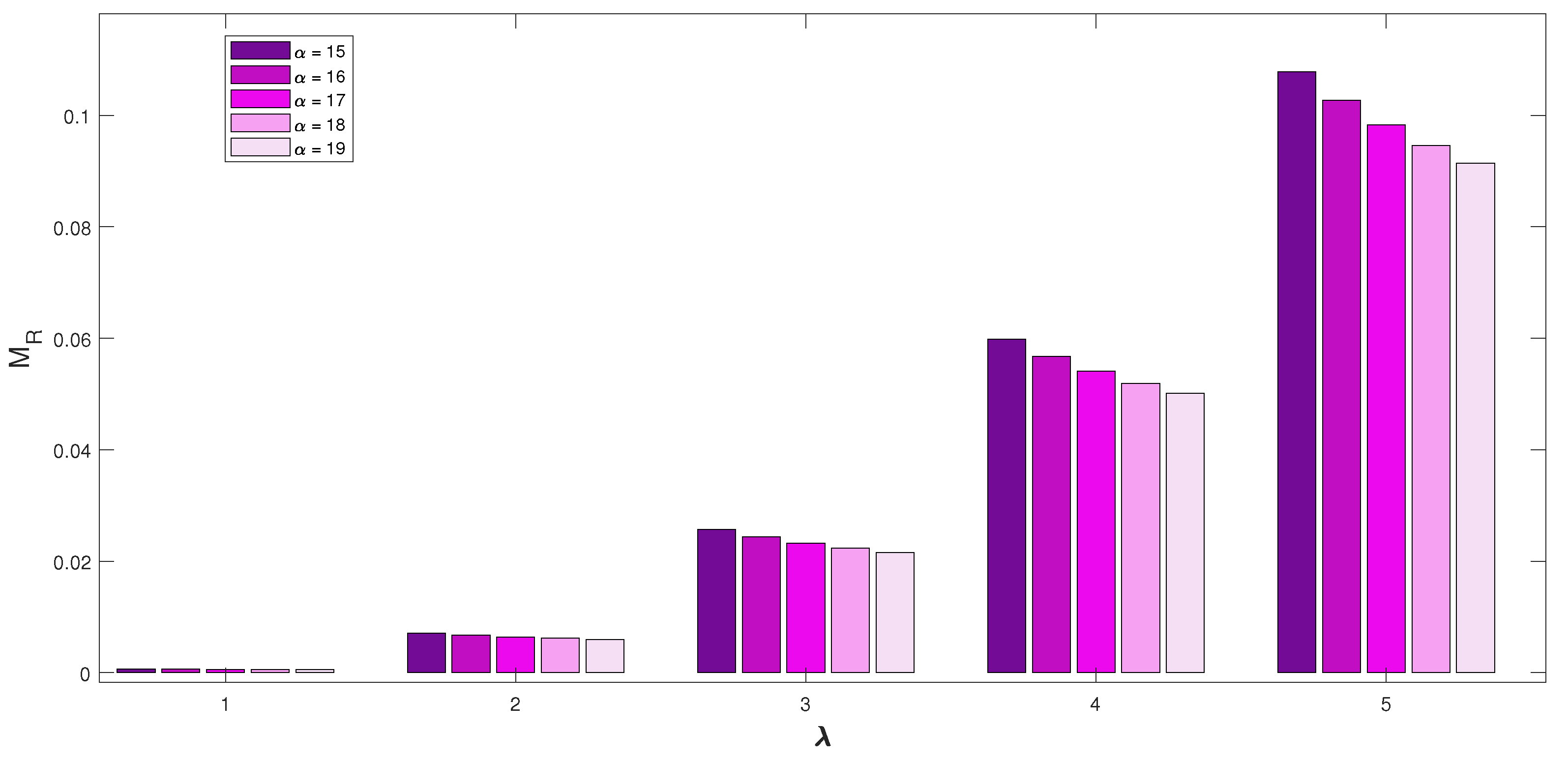
• The repercussions of $\lambda$ and $\alpha$ on $M_R$ are shown in Figure 2. As the service rate $\left(\alpha \right)$ increases, the corresponding mean reorder rate $\left(M_R\right)$ decreases, for each arrival rate $\lambda$. In turn, as the arrival rate increases, the mean reorder rate also increases for each service rate because the reordering depends on the service rate and arrival rate.
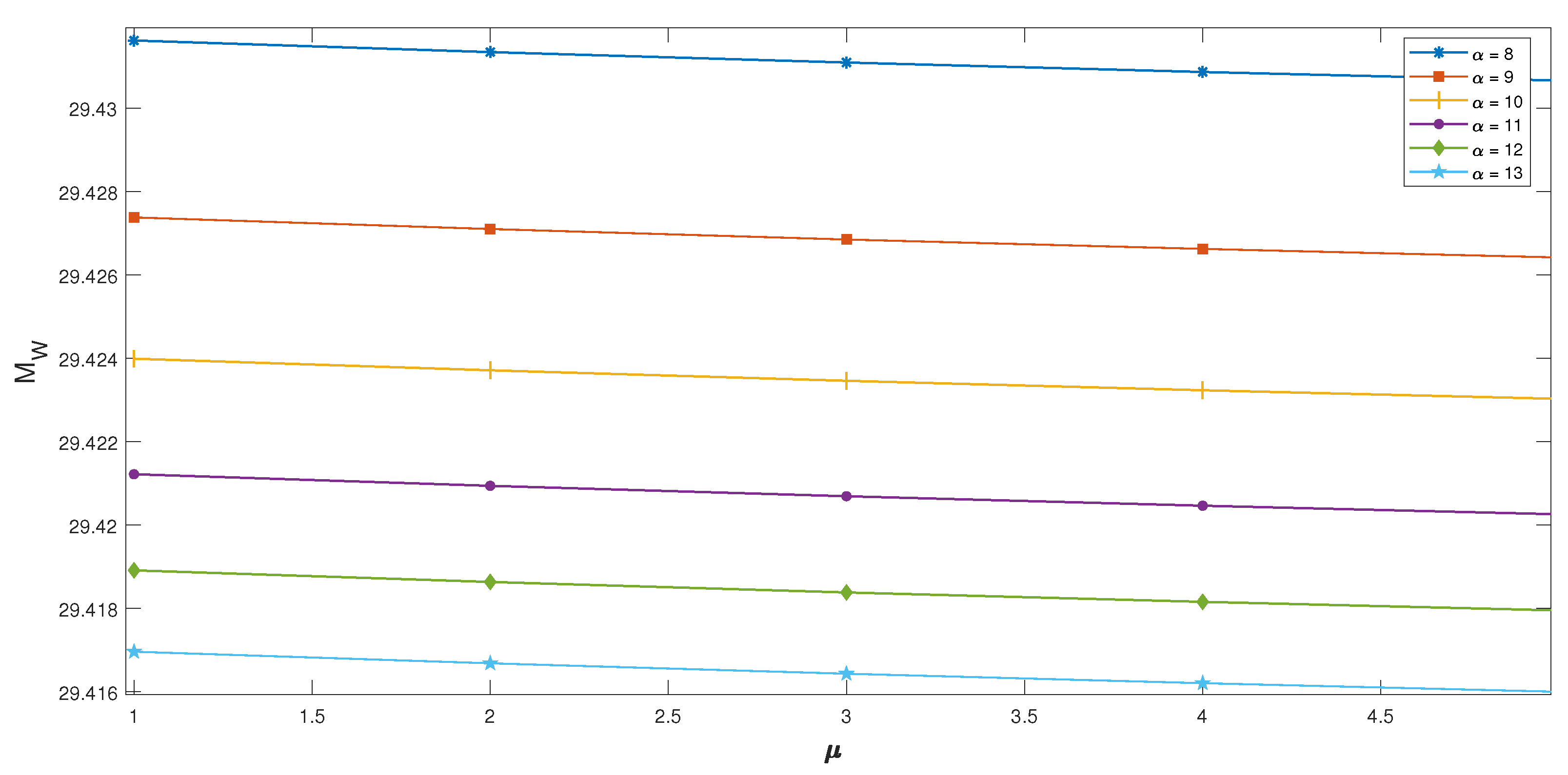
• In Figure 3, we discussed the repercussion on $M_W$ by the rates $\mu$ and $\alpha$. The figure shows that for each reorder rate $\left(\mu \right)$, the mean number of customers in the waiting space $\left(M_W\right)$ has slightly increased as the service rate $\left(\alpha \right)$ increases. And also for each service rate, the mean number of customers in the waiting space decreases very slightly as the reorder rate increases.
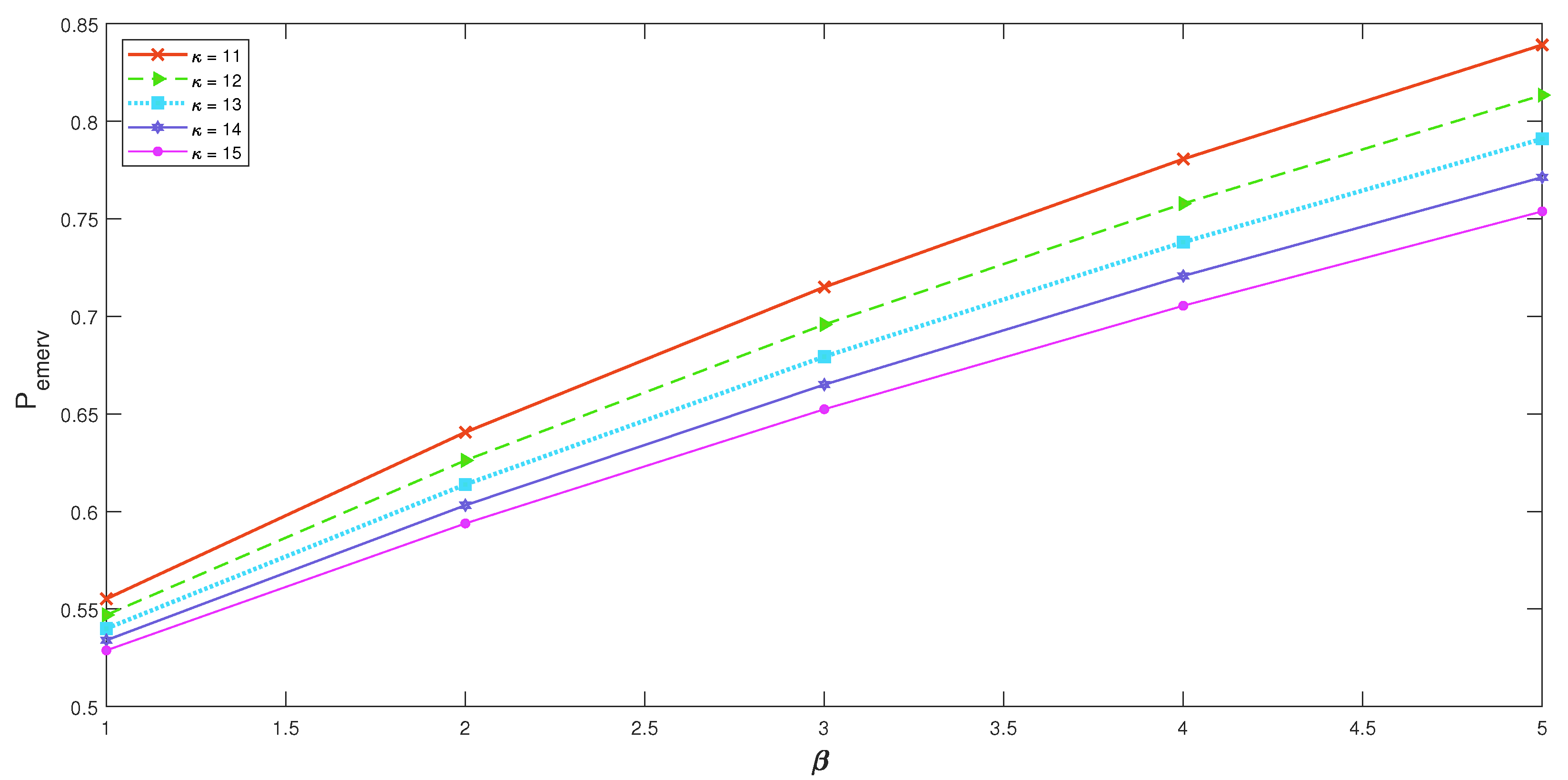
• We demonstrated the repercussion of $\beta$ and $\kappa$ on $P_{emerv}$ graphically in Figure 4. The graph shows that as the parameter of the occurrence of an emergency situation $\left(\beta \right)$ increases, the probability of the server going on an emergency vacation $\left(P_{emerv}\right)$ increases for each value of the emergency vacation rate $\left(\kappa \right)$. Similarly, for each value of $\beta$, the value of $P_{emerv}$ decreases as the value of $\kappa$ increases.
• Figure 5 explains the repercussion on $M_{Im}$ by the parameters $\alpha$ and $\theta$. When the retrial rate $\left(\theta \right)$ increases, the mean value of an impatient customer $\left(M_{Im}\right)$ decreases for each service rate $\left(\alpha \right)$. That means the inter-retrial time becomes small when the rate increases, leading the customers to becoming less impatient while staying in orbit, and this can also depend on the number of customers in orbit. For each retrial rate, the mean impatient value very slightly decreases as the service rate increases.
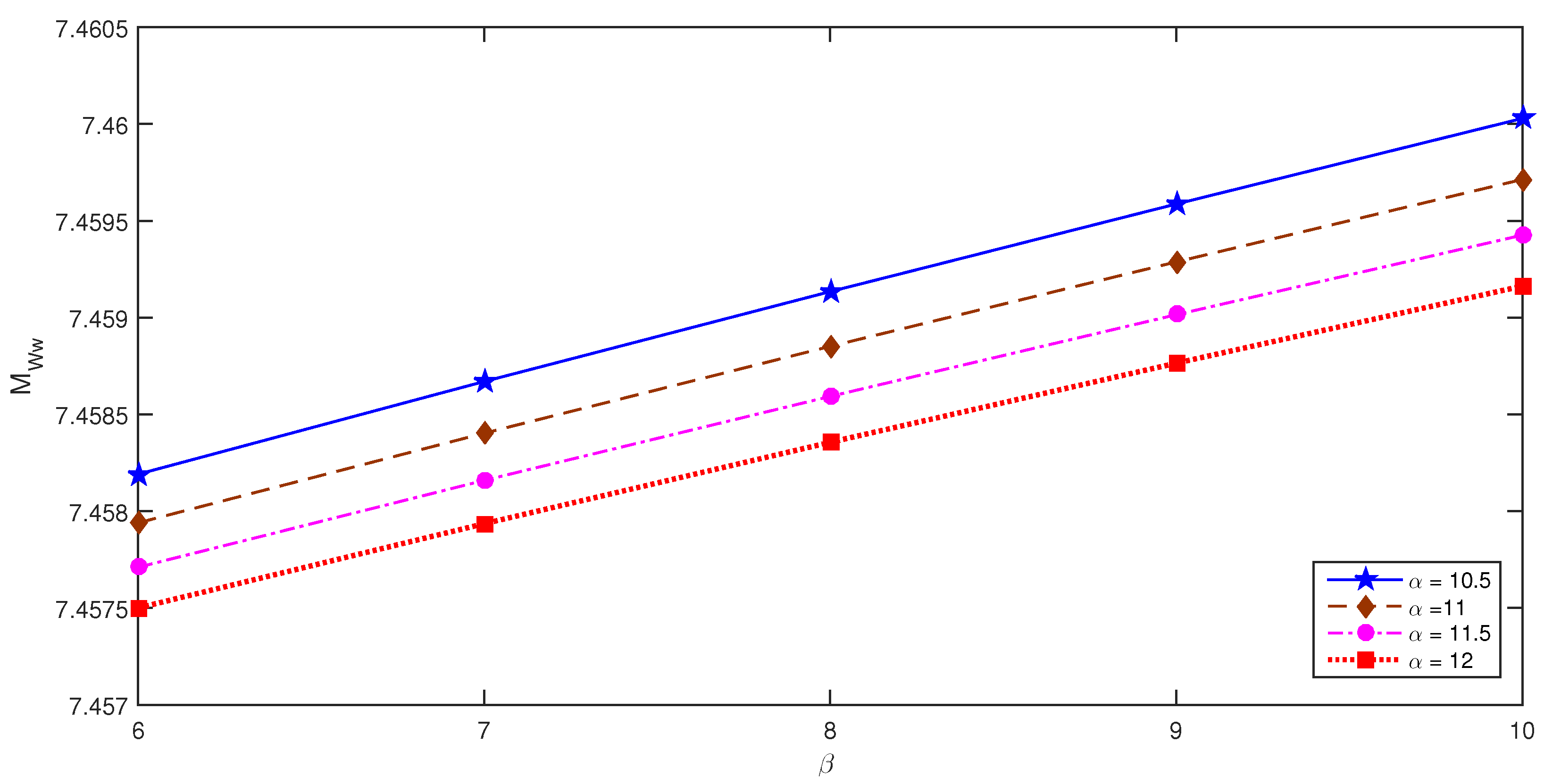
• Figure 6 explains the effect of $\alpha$ on $M_{Ww}$ with respect to different values of $\beta$. The graph shows that as the parameter of the arrival of essential interruptions $\left(\beta \right)$ increases, the average waiting time of the customers in the waiting space $\left(M_{Ww}\right)$ increases for each value of service rate $\left(\alpha \right)$. That means when the occurrence of an essential interruption increases, it increases the waiting time of the customers in the waiting space. Similarly, for each value of the occurrence of an essential interruption, the average waiting time of customers in the waiting space decreases slightly as the service rate increases.

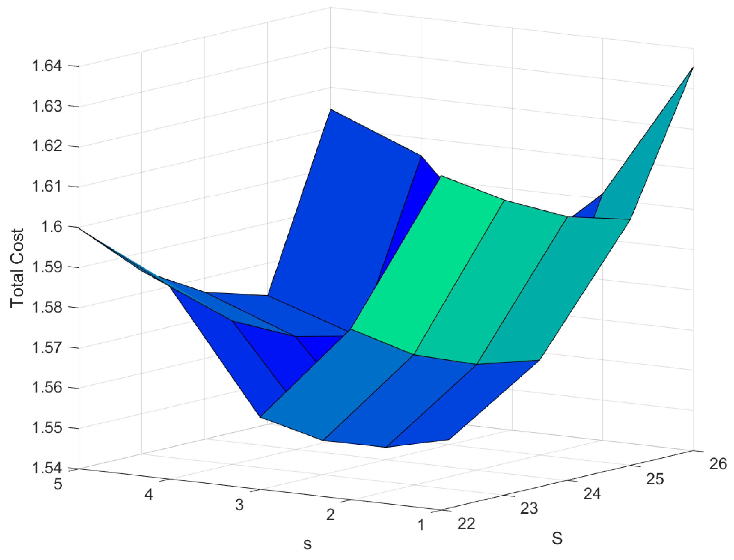
7. Cost Analysis

Using the inventory levels, reorder level, waiting room capacity, and threshold value, as well as incorporating the system’s numerous performance indicators, the total cost function of the interpreted system has also been created.

$$TC(S,s,H,F)=C_h\ast M_I+C_s\ast M_R+C_w\ast M_W+C_o\ast M_O+C_v\ast P_{emerv}+C_l\ast M_{Im};$$

where

• C_h: The holding cost per unit inventory per unit time;
• C_s: The ordering cost of an item per order;
• C_w: The waiting cost of customers in a waiting space per unit time;
• C_o: The waiting cost of an orbiting customer per unit time;
• C_v: Cost per unit time spent by the server in emergency vacation;
• C_l: Cost of a lost customer from the orbit due to impatience.

Table 1. Convexityof total cost.

S/s	4	5	6	7	8
22	1.62314	1.58248	1.55802	1.58798	1.59981
23	1.61340	1.57238	1.54848	1.57566	1.58554
24	1.60556	1.56629	1.54310	1.56807	1.57655
25	1.60120	1.56368	1.54131	1.56452	1.57199
26	1.63544	1.60133	1.58172	1.60557	1.61463

provides the values of the total expected cost function for each pair of S and s values. That is, the minimum value of each row and column were highlighted through bold and underline, respectively. Both bold and underlined value $TC(25,6,5,3)$ = 1.54131 is the local minimum of the total expected cost value of the function $TC(S,s,H,F)$ and it is denoted by $T{C}^{\ast }$. The parameter values which are used to find the optimal value are $\lambda =0.25;\alpha =10.1;\theta =12;\beta =7;\kappa =10;\eta =8;\gamma =1;p=0.5;q=1-p$. The cost values are $C_h=0.01;C_s=2.5;C_w=0.005;C_o=0.5;C_v=1.5;C_l=0.005$; and $N=50$. The graphical structure of the convexity of the total expected cost function is also provided in Figure 7. In

Table 2. Local minimum of the total expected cost ($T{C}^{\ast }$) for various MAPs with corresponding S and s values.

Arrivals	${\mathit{TC}}^{\ast }$
MAP with HEX	25	6
	1.51374
MAP with Erlang	25	6
	1.52501
MAP with PC	25	6
	1.44390
MAP with NC	25	6
	1.44877

, we show the local minimum of the total expected cost $T{C}^{\ast }$ for various MAP arrivals.

8. Conclusions and Future Works

In this article, we studied retrial queueing–inventory system with controlled arrivals experiencing an essential interruption that leads to an emergency vacation, which was motivated by the recent experiences of retailers. We found the steady-state vectors for the considered system and claimed the joint distribution for the quintuplets of the above-given Markov process. We also provided the performance measures of the system. In the numerical illustration, we gave some graphical representations of the sensitivity analysis that has been conducted on the parameters. We found the optimal value of the inventory level $‘S^{\prime }$ and the reorder level ‘s’ using the total cost function and the graph for the convexity of the total cost. In the future, we plan to expand this concept to various real-life situations with other concepts.

References

1. Anbazhagan, N.; Joshi, G.P.; Suganya, R.; Amutha, S.; Vinitha, V.; Shrestha, B. Queueing-Inventory System for Two Commodities with Optional Demands of Customers and MAP Arrivals. Mathematics 2022, 10, 1801. [Google Scholar] [CrossRef]
2. Jeganathan, K.; Selvakumar, S.; Saravanan, S.; Anbazhagan, N.; Amutha, S.; Cho, W.; Joshi, G.P.; Ryoo, J. Performance of Stochastic Inventory System with a Fresh Item, Returned Item, Refurbished Item, and Multi-Class Customers. Mathematics 2022, 10, 1137. [Google Scholar] [CrossRef]
3. Samanta, S.K.; Isotupa, K.S.; Verma, A. Continuous review (s, Q) inventory system at a service facility with positive order lead times. Ann. Oper. Res. 2023. [Google Scholar] [CrossRef]
4. Gupta, S.M. Interrelationship between controlling arrival and service in queueing systems. Comput. Oper. Res. 1995, 22, 1005–1014. [Google Scholar] [CrossRef]
5. Wang, K.H.; Yang, D.Y. Controlling arrivals for a queueing system with an unreliable server: Newton-Quasi method. Appl. Math. Comput. 2009, 213, 92–101. [Google Scholar] [CrossRef]
6. Yang, D.Y.; Wang, K.H.; Wu, C.H. Optimization and sensitivity analysis of controlling arrivals in the queueing system with single working vacation. J. Comput. Appl. Math. 2010, 234, 545–556. [Google Scholar] [CrossRef]
7. Chang, C.J.; Chang, F.M.; Ke, J.C. Economic application in a Bernoulli F-policy queueing system with server breakdown. Int. J. Prod. Res. 2014, 52, 743–756. [Google Scholar] [CrossRef]
8. Chang, C.J.; Ke, J.C.; Huang, H.I. The optimal management of a queueing system with controlling arrivals. J. Chin. Inst. Eng. 2011, 28, 226–236. [Google Scholar] [CrossRef]
9. Jain, M.; Sanga, S.S. State dependent queueing models under admission control F-policy: A survey. J. Ambient Intell. Humaniz. Comput. 2020, 11, 3873–3891. [Google Scholar] [CrossRef]
10. Ke, J.C.; Chang, C.J.; Chang, F.M. Controlling arrivals for a Markovian queueing system with a second optional service. Int. J. Ind. Eng. 2010, 17, 48–57. [Google Scholar]
11. Jain, M.; Shekhar, C.; Shukla, S. Queueing analysis of machine repair problem with controlled rates and working vacation under F-policy. Proc. Natl. Acad. Sci. India Phys. Sci. 2016, 86, 21–31. [Google Scholar] [CrossRef]
12. Nithya, N.; Anbazhagan, N.; Koushick, B.; Amutha, S.; Jeganathan, K. Working Vacation in Queueing-Stock System with Delusive Server. Glob. Stoch. Anal. 2021, 8, 61–80. [Google Scholar]
13. Rani, S.; Jain, M.; Meena, R.K. Queueing modeling and optimization of a fault-tolerant system with reboot, recovery, and vacationing server operating under admission control policy. Math. Comput. Simul. 2023, 209, 408–425. [Google Scholar] [CrossRef]
14. Zhang, Y.; Yue, D.; Yue, W. A queueing-inventory system with random order size policy and server vacations. Ann. Oper. Res. 2022, 310, 595–620. [Google Scholar] [CrossRef]
15. Shekhar, C.; Varshney, S.; Kumar, A. Optimal control of a service system with emergency vacation using bat algorithm. J. Comput. Appl. Math. 2020, 364, 112332. [Google Scholar] [CrossRef]
16. Ayyappan, G.; Thamizhselvi, P. Transient Analysis of M[X1],M[X2]/G1,G2/1 Retrial Queueing System with Priority Services, Working Vacations and Vacation Interruption, Emergency Vacation, Negative Arrival and Delayed Repair. Int. J. Comput. Math. 2018, 4, 1–35. [Google Scholar]
17. Ayyappan, G.; Udayageetha, J. Retrial Queueing System with Priority Services, Working Breakdown, Non-Persistent Customers, Modified Bernoulli Vacation, Emergency Vacation and Repair. Int. J. Stat. Syst. 2018, 13, 23–39. [Google Scholar]
18. Vaishnawi, M.; Upadhyaya, S.; Kulshrestha, R. Optimal Cost Analysis for Discrete-Time Recurrent Queue with Bernoulli Feedback and Emergency Vacation. Int. J. Comput. Math. 2022, 8, 1–31. [Google Scholar] [CrossRef]
19. Krishnamoorthy, A.; Nair, S.S.; Narayanan, V.C. An inventory model with server interruptions and retrials. Oper. Res. 2012, 12, 151–171. [Google Scholar] [CrossRef]
20. Krishnamoorthy, A.; Nair, S.S.; Narayanan, V.C. Production inventory with service time and interruptions. Int. J. Syst. Sci. 2015, 46, 1800–1816. [Google Scholar] [CrossRef]
21. Fiems, D.; Maertens, T.; Bruneel, H. Queueing systems with different types of server interruptions. Eur. J. Oper. Res. 2008, 188, 838–845. [Google Scholar] [CrossRef]
22. Ke, J.C. The optimal control of an M/G/1 queueing system with server vacations, startup and breakdowns. Comput. Ind. Eng. 2003, 44, 567–579. [Google Scholar] [CrossRef]
23. Wu, J.; Lian, Z. A single-server retrial G-queue with priority and unreliable server under Bernoulli vacation schedule. Comput. Ind. Eng. 2013, 64, 84–93. [Google Scholar] [CrossRef]
24. Xu, J.; Hou, I.-H.; Gautam, N. Age of information for single user system with vacation server. IEEE Trans. Netw. Sci. Eng. 2022, 9, 11981214. [Google Scholar] [CrossRef]
25. Anbazhagan, N. Stochastic Inventory System with Compliment Item and Retrial Customers. In Stochastic Processes and Models Operations Research; IGI Global: Hershey, PA, USA, 2016; pp. 148–164. [Google Scholar]
26. Anbazhagan, N.; Jeganathan, K. Two-commodity Markovian inventory system with compliment and retrial demand. Brit. J. Math. Comput. Sci. 2013, 3, 115–134. [Google Scholar] [CrossRef] [PubMed]
27. Melikov, A.Z.; Shahmaliyev, M.O. Queueing System M/M/1/ with Perishable Inventory and Repeated Customers. Autom. Remote 2019, 80, 53–65. [Google Scholar] [CrossRef]
28. Al Hamadi, H.M.; Sangeetha, N.; Sivakumar, B. Optimal control of service parameter for a perishable inventory system maintained at service facility with impatient customers. Ann. Oper. Res. 2015, 233, 3–23. [Google Scholar] [CrossRef]
29. Chakravarthy, S.R. Markovian arrival processes. In Wiley Encyclopedia of Operations Research and Management Science; Wiley: Hoboken, NJ, USA, 2010. [Google Scholar]
30. Neuts, M.F. Matrix-Geometric Solutions in Stochastic Models: An Algorithmic Approach; Dover Publication: New York, NY, USA, 1994. [Google Scholar]
31. Neuts, M.F.; Rao, B.M. Numerical investigation of a multiserver retrial model. Queueing Syst. 1990, 7, 169–189. [Google Scholar] [CrossRef]
32. Chakravarthy, S.R.; Krishnamoorthy, A.; Joshua, V.C. Analysis of a multi-server retrial queue with search of customers from the orbit. Perform. Eval. 2006, 63, 776–798. [Google Scholar] [CrossRef]
33. Latouche, G.; Ramaswami, V. A Logarithmic Reduction Algorithm for Quasi-Birth-Death Processes. J. Appl. Probab. 1993, 30, 650–674. [Google Scholar] [CrossRef]
34. Ross, S.M. Introduction to Probability Models; Harcourt Asia PTE Ltd.: Singapore, 2000. [Google Scholar]
Figure 1. Repercussions of arrival rate λ and retrial rate θ on M O .
Mathematics 11 03560 g001
Figure 2. Repercussions of α and λ on M R .
Mathematics 11 03560 g002
Figure 3. Repercussions of α and μ on M I m .
Mathematics 11 03560 g003
Figure 4. Repercussions of β and κ on P e m e r v .
Mathematics 11 03560 g004
Figure 5. Repercussions of α and θ on M I m .
Mathematics 11 03560 g005
Figure 6. Repercussions of α and β on M W w .
Mathematics 11 03560 g006
Figure 7. Convexity of total cost.
Mathematics 11 03560 g007