Survey of Point Cloud Registration Methods and New Statistical Approach

Abstract

The use of a 3D range scanning device for autonomous object description or unknown environment mapping leads to the necessity of improving computer methods based on identical point pairs from different point clouds (so-called registration problem). The registration problem and three-dimensional transformation of coordinates still require further research. The paper attempts to guide the reader through the vast field of existing registration methods so that he can choose the appropriate approach for his particular problem. Furthermore, the article contains a regression method that enables the estimation of the covariance matrix of the transformation parameters and the calculation of the uncertainty of the estimated points. This makes it possible to extend existing registration methods with uncertainty estimates and to improve knowledge about the performed registration. The paper’s primary purpose is to present a survey of known methods and basic estimation theory concepts for the point cloud registration problem. The focus will be on the guiding principles of the estimation theory: ICP algorithm; Normal Distribution Transform; Feature-based registration; Iterative dual correspondences; Probabilistic iterative correspondence method; Point-based registration; Quadratic patches; Likelihood-field matching; Conditional random fields; Branch-and-bound registration; PointReg. The secondary purpose of this article is to show an innovative statistical model for this transformation problem. The new theory needs known covariance matrices of identical point coordinates. An unknown rotation matrix and shift vector have been estimated using a nonlinear regression model with nonlinear constraints. The paper ends with a relevant numerical example.

1. Introduction

In the registration problem, data describing a certain object in different coordinate systems is available. This arises quite naturally if we measure points on the object from different positions. We thus obtain so-called clouds of points in individual scans. When solving the registration problem, we search for matching (identical) points in different scans and estimate the transformation parameters. The criterion for estimating unknown parameters is often the minimization of the alignment error. Pioneering methods for solving the registration problem were developed in the 1980s in the field of 2D image matching. This important problem of computer graphics crystallized, especially during the processing of medical images. Research gradually moved towards the application of 3D point cloud registration. Applications in object reconstruction, non-contact inspections, medical and surgery support, robot navigation, and autonomous vehicle navigation gradually appeared. An overview of methods used in 2D registration is published in the book [1]. The paper [2] contains a literature survey on the use of the registration problem in robotics and robot navigation. The state-of-the art of registration problem with an emphasis on radar data is dealt with in the book [3].

Nowadays, laser scanning is finding huge use. A comprehensive review of terrestrial laser scanner (TLS) point cloud registration methods is given in ref. [4]. The book [5] expressed the TLS as follows: “TLS systems enable documentation of the whole measured object with all constructional elements. The high scanning speed of the current scanners enables a significant reduction in the time necessary for measurement and, alternatively, an increasing amount of information about the measured object. More data (several million points) enable the creation of complex models or documentation of objects in the form of a detailed point cloud”. A relatively large potential for the use of such models has arisen. As such, laser scanning finds application in various fields: industry, robotics, process control, quality control, architecture, civil engineering, archeology, geosciences, medical sciences, and dentistry. Autonomous laser scanning systems also offer the prospect of saving human lives. They are deployed in dangerous environments such as unexplored areas, abandoned places, or mines. Such systems offer the possibility of getting detailed maps of the unknown surrounding environment without human intervention. In these systems, solving registration problems is crucial. Cf. [5].

Our measurement was made by using an optical rangefinder, which uses an optical filter to spread the green laser beam in a vertical line. See Figure 1. At each detected point of this line, it is possible to determine a 3D point in the scanned environment. Figure 2 demonstrates laser scanning of an indoor room. The optical rangefinder’s measurement head is rotating in 360 degrees around the Z axis to scan the whole surrounding area. The resulting point clouds form two positions and are presented in Figure 3. Using a camera, you can create a colored point cloud.

In this paper, we will mainly discuss methods applicable to 3D registration. In doing so, we will focus on the registration of building objects. Firstly, we present an overview of the most commonly used methods. In addition, we will propose a statistical algorithm that can become an appendix to standard algorithms. In the model, we will assume that the transformation is formed only by shift and rotation in 3D space. Such a transformation is sometimes referred to as a rigid transformation. In this new algorithm, we will consider measurement errors in individual scans. This regression model will allow the synchronous estimation of unknown transformation parameters from all scans. The prerequisite for using this approach will be the knowledge of identical points. These points can be earned through standard registration methods. In special geodetic problems, points on the object can be given by placing reflective targets, which are then focused in individual scans. Here, it is not necessary to look for identical points, as they are determined by reflection points.

Let us return to the description of an example of a typical 3D registration problem. Measured coordinates of points are given in the point clouds, which can be obtained from different scans from different positions. Figure 3 gives a point cloud registration example. The registration problem’s aim is to create a compact point cloud with all possible details.

The structure of the article is as follows. In the introductory chapter, the framework of existing knowledge was outlined, the assumptions and goals of the proposed statistical model were described, and the realization of a specific laser measurement was presented. The second section seeks to examine and discuss the main currents of thought in the theoretical and practical solution of registration problems without attempting to present the details of all the methods. In the third chapter, we will state a new statistical method, which exploits a regression model with constraints. In the fourth chapter, a concluding discussion is made.

A fundamental shortcoming of commonly used methods is the fact that the covariance matrices of the measured points are often not used or are replaced by identical matrices. Further, the estimate of the variance matrix of the estimated coordinates is not known. We find this estimate using an indirect measurement regression model with a system of nonlinear constraints. Separately, this model is applicable in the case of geodetic measurements, when identical points are marked with reflective targets. After gaining pairs of identical points from commonly used methods, the new approach will find application in the process of object modeling.

1.1. Optical Rangefinder

The principles of the 3D technique for object description are based on the triangulation method. The idea of measuring the distance and then determining the point cloud is mentioned in the article [6]. A rotating tripod carried the entire measuring device; see Figure 1. A Basler camera with an output of 2590 × 1942 pixels was used to capture the image in high quality. The output power of 200 mW of the used laser diode made it possible for good recognition after vertical swapping. An optical filter with a 90-degree angle scattered the laser spot. A powerful and fast-stepping motor enabled the measuring head to rotate 360 degrees. Captured colored images are processed by image processing methods to get precise laser line determination in the individual scanned images. For each detected point on the line, the 3D position in the surrounding scanning area is calculated. Image information is also used in the point cloud creation process to get a colored point cloud; see ref. [6].

1.2. 3D Point Cloud

The Figure 2 left side shows an example of the implementation of one frame measurement. Laser line segmentation was performed using a green-colored Gaussian Mixture Model (GMM). For more details, see the article [6]. By using laser mask analysis, 10 different distances were measured. The total number of N measured points in one image was 80. The mobile device is located at the coordinates $P=(P_X,P_Y,P_Z)$. The point P is the origin of one automatic 360-degree scan. Through measurement data processing, the 3D point cloud is created. An example of a 3D point cloud is in Figure 3. The used coordinate system is Cartesian, and each point in this point cloud is described by a vector $p=(p_X,p_Y,p_Z)$, where $p_X$, $p_Y$, and $p_Z$ are coordinates in the appropriate axis.

The black dot marks mobile platform position $P_1$. This point cloud covers the measurement from one position, and there are some important points missing in the top corner. The whole scanning process’s intention is to create a compact map of a scanning space. For this purpose, it is necessary to provide the measurement from more positions in a scanning space. For changing the measurement position, the used measurement device can be, for example, placed manually in a new position or mounted on a mobile device, which provides precise information about its position in space. We place a mobile platform manually in a scanning environment. The differences in position we measure with the precise laser rangefinder.

2. A Survey of Methods

In the following subsections, we will present the ideas of the most commonly used methods developed to solve the registration problem.

2.1. ICP Algorithm

ICP is the oldest registration algorithm; cf. [7,8]. If the user’s measurement or device’s localization is accurate, the registration can be determined directly by separate measurements. Figure 3 describes the connection to one group. However, imprecise measurement sensors and erroneous self-localization have to be assumed for registration. The frequently used method is called Iterative Closest Points (ICP); see refs. [9,10].

Let’s have two independently gained sets of 3D points, the measurement from position $P_1$ and $P_2$, we want to estimate the transformation $(\mathbf{R},\mathbf{t})$ forming by a rotation matrix $\mathbf{R}$ and a shift vector $\mathbf{t}$ which minimizes the cost functional

$$\begin{array}{ccc}\hfill E(\mathbf{R},\mathbf{t})& =& \sum _{i=1}^{N_m}\sum _{j=1}^{N_d}{w}_{(}i,j\left)\right||{\widehat{m}}_i-\left(\mathbf{R}{\widehat{d}}_j\right)+\mathbf{t}{\left|\right|}^2.\hfill \end{array}$$

(1)

The parameter $w_{i,j}$ takes the value 1 when the i-th point of $\widehat{M}$ determines the same 3D position of the point as the j-th point of $\widehat{D}$. If it specifies another point, then $w_{i,j}$ is 0. Next, two parameters need to be determined: the corresponding points and the function $E(\mathbf{R},\mathbf{t})$ that minimizes $E(\mathbf{R},\mathbf{t})$ with the use of corresponding points. The ICP algorithm iteratively computes the point correspondences. In each step of the algorithm, the algorithm searches the closest points as correspondences and computes the transformation $(\mathbf{R},\mathbf{t})$ for the minimizing value $E(\mathbf{R},\mathbf{t})$.

2.1.1. ICP Algorithm Results

The ICP algorithm application result is shown in Figure 4, and the final RMS value between both point clouds is 0.167. The point cloud contains points from the second measurement that fill the empty area in the first measurement (top corner). The new point cloud contains more measurement points and gives more details about the scanned room. In Figure 4, on the left side are both registered point clouds from Figure 3. On the right side, there is a colored version.

2.1.2. ICP Algorithm Problem

By using the ICP method, there are two main problems. The ICP algorithm is point-based, and it does not take into account the local surface and shape around each point. The ICP algorithm is also time-consuming in searching for the nearest neighbor. Even if an efficient search data structure such as a kd-tree is used, the estimation time for a large number of points is long. If both scans are with a bigger distance offset and rotated in all axes by about several tens of degrees, the registration result is obtained with error.

2.2. Normal Distribution Transform (NDT)

The method was proposed in the publication [11]. The basic pillar of this algorithm is the capture of data by a statistical model. The method does not focus on the simple use of individual measurement points but instead constructs a model of mixtures of normal distributions and examines the probabilities of the surface point occurring in a certain position; see ref. [12]. This approach provides a piece-wise smooth introduction to the point cloud model with continuous first- and second-order derivatives. This representation is followed by standard numerical optimization methods for the registration problem. The NDT algorithm consists of several steps: firstly, the whole point cloud is dismembered into small subdomains (cells), and for each cell, statistical characteristics such as the mean and the covariance matrix are computed. We consider that the coordinates of the reference scan surface points have a D-dimensional normal distribution. The likelihood function is

$$\begin{array}{cc}& p\left(\mathbf{x}\right)=\frac{1}{{\left(2\pi \right)}^{\frac{D}{2}}\sqrt{\left|\mathsf{\Sigma }\right|}}exp\left(-\frac{1}{2}{(\mathbf{x}-\mathbf{\mu })}^{\prime }\mathsf{\Sigma }(\mathbf{x}-\mathbf{\mu })\right),\end{array}$$

(2)

where $\mathbf{\mu }$ is the vector of mean values and $\mathsf{\Sigma }$ is the covariance matrix of the reference points on the scanned surface in the cell in which $\mathbf{x}$ is located. The constant $c_0$ denotes the expression ${\left(2\pi \right)}^{\frac{D}{2}}\sqrt{\left|\mathsf{\Sigma }\right|}$. The estimates of the mean and covariance matrix are

$$\begin{array}{ccc}\hfill \overline{\mathbf{\mu }}& =& \frac{1}{m}\sum _{k=1}^m{\mathbf{y}}_k,\hfill \end{array}$$

(3)

$$\begin{array}{ccc}\hfill \overline{\mathsf{\Sigma }}& =& \frac{1}{m-1}\sum _{k=1}^m({\mathbf{y}}_k-\mathbf{\mu }){({\mathbf{y}}_k-\mathbf{\mu })}^{\prime },\hfill \end{array}$$

(4)

where ${\mathbf{y}}_k$, $k=1,\dots ,m$ are coordinates of reference scan points form a cell. According to the eigenvalues of the covariance matrix, it is possible to estimate the shape of the cell. This will help in the point cloud registration process. In the NDT method, we look for such a position of the actual scan that when the maximum probability occurs, the points of the actual scan are located on the surface of the reference scan. Searched Helmert transformation parameters (i.e., translation and rotation) offer a pose estimate in the given scan; for encoding, we will use the vector variable p. In the current scan, we have point clouds $X=\{{\mathbf{x}}_1,\dots ,{\mathbf{x}}_n\}$.

The displacement of the point $\mathbf{x}$ in space by the position $\mathbf{p}$ is described by the spatial transformation function $T(\mathbf{p},\mathbf{x})$. We consider the best estimate of the true position $\mathbf{p}$ to be the one that maximizes the likelihood

$$\begin{array}{ccc}\hfill L& =& \prod _{k=1}^{n}p\left(T(\mathbf{p},{\mathbf{x}}_k)\right).\hfill \end{array}$$

(5)

For 3D-NDT registration, the Euler angles are useful because of their natural advantages. This representation does not need a numerical optimization procedure with easier-to-calculate derivatives. If we use the representation using Euler angles, there are six transformation parameters to estimate: three unknown translation parameters and three unknown rotation parameters. The rotation matrix can be expressed by Cardan angles and angles of yaw, pitch, and roll, ref. [13]. The pose can be explained using the six-dimensional vector ${\mathbf{p}}_6={[t_x,t_y,t_z,{\varphi }_x,{\varphi }_y,{\varphi }_z]}^{\prime }$ using the Euler angles. Then the 3D transformation is given by formula:

$$\begin{array}{ccc}& T_E({\mathbf{p}}_6,\mathbf{x})=\mathbf{R}\mathbf{x}+\mathbf{t}={\mathbf{R}}_x{\mathbf{R}}_y{\mathbf{R}}_z{\mathbf{x}}_k+\mathbf{t},& \\ & \mathbf{R}=\left(\begin{array}{ccc}{c}_x{c}_z& -c_y{s}_z& s_y\\ c_x{c}_z+s_x{s}_y{c}_z& c_x{c}_z-s_x{s}_y{c}_z& -s_x{c}_y\\ s_x{s}_z-c_x{s}_y{c}_z& c_x{s}_y{s}_x+s_x{c}_z& c_x{c}_y\end{array}\right),& \\ & \mathbf{t}={(t_x,t_y,t_z)}^{\prime }\end{array}$$

(6)

where $c_i=cos{\varphi }_i$ and $s_i=sin{\varphi }_i$.

2.3. Feature Based Registration

The feature-based matching extracts distinguishing features from the range of images and uses corresponding features to calculate scan alignment. For most robots, the detection of closed loops is realized from camera data [14]. The most common functions of the detector are: SURF; SIFT; GLOH; Shape Context; PCA; Moments; Cross-correlation; and Steerable filters [9]. A major aspect of feature detectors is their invariance with individual transformation parameters: scale, shift, rotation, and illumination changes. A comprehensive survey of detectors and descriptors is given in [15]. These methods use the Gaussian function for image spectral analysis

$$\begin{array}{ccc}\hfill G(x,y,\sigma )& =& \frac{1}{2\pi {\sigma }^2}exp\left(\frac{x^2+y^2}{2{\sigma }^2}\right),\hfill \end{array}$$

(7)

where x and y are pixel coordinates in an image, and $\sigma$ is the Gaussian parameter. The n-times filtration provides scale invariance. The input images of the convolution with variable scales give the differences of Gaussian (DoG), which are the image features. For a significant increase in computation speed, the SURF method uses Gaussian function approximation. The feature-based navigation system is presented in ref. [16]. The autonomous robot is guided along a given path. The navigation is based on exteroceptive sensors, and a simple, effective mathematical model is suitable.

2.4. IDC

The iterative dual correspondence (IDC) algorithm [17] can be considered an extension of ICP. The main mission is to accelerate the convergence of the rotation matrix when estimating position in scan registration. In this method, two rules are introduced to determine the correspondence. The first is similar to the ICP. In each iteration, the rotation and translation pair ${\tau }_1$ are determined using the closest points. The second criterion, called ’the matching range-point rule’ deals with the point selection of a new set of corresponding points. In this criterion, corresponding points are identified within the permissible angular interval. An equation in 2D space has the form $[\phi -t_{\phi },\phi +t_{\phi }]$, $t_{\phi }$ and is limited (how far the algorithm should seek). The matching range-point metric is determined as follows: $\mathrm{corresponding}\left(\mathbf{x}\right)={\arg \min }_{{\mathbf{x}}^{\prime }}\left(\right|r-\rho \left|\right)$ where $\mathbf{x}=[\phi ,r]$ and ${\mathbf{x}}^{\prime }=[\varphi ,\rho ]$, and $\varphi -t_{\varphi }\le \rho \le \varphi +t_{\varphi }$.

The corresponding point is located within the specified angular limits. In 3D space, an interval is a cuboid-shaped “window” whose projections into the planes are rectangles. A three-dimensional point $\mathbf{x}$ is given by polar coordinates $[\varphi ,\theta ,r]$, where $\varphi$ and $\theta$ are the latitude and longitude angles. This window is bound from $[\varphi -t_{\varphi },\theta -t_{\theta }]$ to $[\varphi +t_{\varphi },\theta +t_{\theta }]$. A comparison of the quality of the solution to the registration problem led to the conclusion that the IDC algorithm is more robust than the ICP. However, with a large bias in the initial estimate of the position compared with the actual value, greater inaccuracies in the solution occurred more with the IDC than with the ICP. The IDC method is much more sensitive to a biased initial solution. Cf. [17].

2.5. pIC

Another approach is a registration algorithm called the probabilistic iterative correspondence method (pIC), cf. [18]. In this algorithm, scan noise data is combined with an initial estimate of position. The coordinates of the scan points and the initial estimate of the position are assumed to be random variables with zero mean Gaussian noise. For the best result from matching, the covariance matrix is based on the sensor positions and robot odometry. In the beginning, points from both scans are selected to create a subset composed of statistically compatible points. The construction of the pairing fitness function is based on the minimization of the Mahalanobis distance $d_m(\mathbf{x},\mathbf{y})$. of point $\mathbf{x}$ and $\mathbf{y}$,

$$\begin{array}{ccc}\hfill d_m^2(\mathbf{x},\mathbf{y})& =& \left|\right|\mathbf{x}-\mathbf{y}\left|\right|{\mathsf{\Sigma }}^{-1}\left|\right|\mathbf{x}-\mathbf{y}\left|\right|\hfill \end{array}$$

(8)

where $\mathsf{\Sigma }$ is a known estimate of the covariance matrix, including sensor properties and system conditions. If the Mahalanobis distance does not exceed the specified threshold, these points are considered compatible. The set of points satisfying this constraint formulates a subset of A. The method for determining the minimum argument of the fitness function, i.e., estimating the point $y_i\in A$ that best corresponds to the point $\mathbf{x}$, is the integration of each admissible locations $\mathbf{x}$ and each admissible sensor coordinates considering their Gaussians estimates.

The results of the pIC algorithm were compared with those of IDC and ICP. pIC estimates were more robust with respect to a biased initial solution.

The pIC method shows faster convergence, about 25 %. Cf. [18].

2.6. Point-Based Probabilistic Registration

In this method, the measured coordinates of the discrete points of the reference scan are replaced by probabilistic functions, cf. [19]. The basis for estimating the probability of a scan point from the current cloud is to trace a ray rising from the estimated position, along the direction associated with each measurement from the current scan, to the nearest surface in the reference scan. Triangulation of the reference coordinate system scan is then performed to create an approximation of the surface. The estimated range of this measurement is determined by the length of the beam.

The likelihood function of a scan point is determined from a mixture of Gaussian values that are centered in an estimated range, with variance determined by known scanner characteristics, and a uniform distribution that is also determined with respect to scanner uncertainties. The probability of the distance r obtained by measurement (the distance to the cloud point $\mathbf{x}$) depends on the theoretical distance (the mean of the Gaussian value). This value is calculated through the mixture model using the Euclidean metric between scan points $\mathbf{x}$ and the triangulated reference scan surface. The calculation uses the expected metric $d_e(\mathbf{x},Y,\mathbf{p})$ pursuant to the direction of the beam $\mathbf{x}$, the reference cloud Y, and the position $\mathbf{p}$. The probability that the position of the current cloud is $\mathbf{p}$ is given by multiplying probabilities ${\prod }_{\mathbf{x}\in X}p\left(\mathbf{x}\right|d_e(\mathbf{x},Y,\mathbf{p}))$.

The algorithm tries to optimize the likelihood function. The presented results by the authors include a pair of building scans in different coordinate systems, and it is discussed that the method gives results with less uncertainty in comparison with the ICP on this data set. Cf. [19].

2.7. Gaussian Fields

The next developed registration method has the name Gaussian fields, cf. [20]. This approach is similar to the Normal Distribution Transformation (NDT). A Gaussian mixture model (GMM) becomes the main tool here for measuring the scan’s statistical characteristics, the spatial distance between the points, and the surface similarity around the points. The comparison of points is realized in a multidimensional space, the dimension of which is given by the spatial dimension of the coordinate system, which is increased by the number of attributes. The proximity and similarity of points $\mathbf{x}$ and $\mathbf{y}$ from different clouds is

$$\begin{array}{ccc}\hfill F(\mathbf{x},\mathbf{y})& =& exp(-\frac{\left|\right|\mathbf{x}-\mathbf{y}\left|\right|}{d_g^2}-{(S\left(\mathbf{x}\right)-S\left(\mathbf{y}\right))}^{\prime }\times \hfill \\ & & {\mathbf{D}}^{-1}(S\left(\mathbf{x}\right)-S\left(\mathbf{y}\right))),\hfill \end{array}$$

(9)

where $S\left(\mathbf{x}\right)$ is the 3D-moment shape characteristics of the surface passing through $\mathbf{x}$. Equation F(x, y) describes a Gaussian function centered at $\mathbf{y}$. The parameter $d_g$ describes the decomposition rate according to the spatial function, and the diagonal matrix $\mathbf{D}$ determines the penalty given by differences in attributes. The fitness function is ${\sum }_{i,j}F(x_i,y_i)$. Cf. [21].

2.8. Quadratic Patches

In this method, the reference scanned surface is expressed implicitly when the approximant is constructed using the square of the distance from the surface. The minimization of the distance metric given by the sum of squared distances defines the criterion to connect points from the current scan. The local shape of the surface is fitted by approximants using quadratic terms, i.e., the second-order derivative. The optimum of this surface representation can be found by Newton’s optimization method. Cf. [22].

2.9. Likelihood-Field Matching

This variant of registration works with similar principles as NDT. The method is often used by developers for 2D sonar scan registration. The large uncertainty of the angular resolution of sonars, compared with lidars, brings complications to the successful identification of registration points. In the method, a sequence of scans is first accumulated using robot odometry to obtain multi-point scans. Such an additional procedure can be applied to the input data for all scan registration algorithms. Thus, a new group of methods was created with the following prefix: sNDT, sICP. The method, named LF/SoG (short for probability field introduced as a sum of Gaussians), is very comparable to NDT when the points in one scan are corrected to a normal distribution according to the points from the next scan. In this method, an identity matrix is used instead of the covariance matrix estimates. Instead of a discrete explicit grid, the entire reference scan is passed through the circular window by replacing the values of the internal points in the sliding window with their centers of gravity. A Gaussian approximant is centered at the point of the resampled cloud, with the mean given by the point pose and the covariance matrix set to the identical matrix. In the process of registration, not only the nearest points are used for the calculation of the optimization criterion but also points at a defined distance from the Gaussian function. Cf. [23].

2.10. CRF Matching

Conditional Random Fields (CRF) is a probabilistic approach used in the construction of relational information models. Unlike hidden Markov models or Markov random fields, the use of CRF does not require independence of observations. Originally, CRFs were implemented in the field of computational linguistics, where they were used to label sentences according to parts of speech. Conditional random fields have been implemented to register 2D scans. In the algorithm, the CRF created for each point in the current scan introduces a hidden node. In turn, each hidden node is assigned to its corresponding point in the reference scan. The hidden node is also linked to a data node that contains certain functions defined for each scan point. On the selected training data, the model learns and searches for suitable parameters. Cf. [24].

2.11. Branch-and-Bound Registration

A branch-and-bound strategy is another registration algorithm presented in [25]. First, the translational part of the position space is discretized in several resolutions with ordered levels from the coarsest to the finest. The sequence of poses is analyzed at a certain level of the hierarchy. At the second lowest hierarchical level (branching), the value of the score is determined, on the basis of which sub-nodes are eliminated (boundary). This application is often used in forestry. The application is suitable for highly unstructured environments. It is particularly interesting in 2D analysis. The branch-and-bound procedure is used in the translation part of the transformation. This method is used in applications aimed at modeling the orientation of the robot based on various sensors. The initial value of the rotation matrix plays an important role here. In a space with six degrees of freedom (position in a space and orientation angles yaw, pitch, and roll angles), the optimization is complicated. Cf. [25].

2.12. Registration Using Local Geometric Features

Compared with the point algorithms described earlier, registration can also be implemented using more descriptive local geometric elements [26]. An ideal local property descriptor is invariant to rigid motion so that the corresponding surface can be found regardless of initial scan positions. The correspondence problem is solved when sufficiently prominent features are found. Furthermore, a global adaptation of the surface is possible, i.e., the realization of registration without an initial estimate of the position. The most commonly used surface description method is ’spin-images’. The spin-image is constructed at an oriented point, which is a surface point with a specified normal vector. Another alternative gives ’surface signatures’. These are similar to spin images but use surface curvature instead of point density. Another alternative surface description is the ’splash’. Spatters are determined around oriented points and involve capturing the point cloud using triangulation methods. All these description techniques are used to express the geometric features of both scans. The main aim is to calculate the estimates of rotation and translation parameters between the scans in such a way that we will obtain their minimal mutual distance. Cf. [26].

2.13. PoitnReg

Another registration approach for a wide range of three-dimensional scans is presented in ref. [27]. This paper deals with the pitfalls of 3D range scans. The rangefinder translates coordinates to a chosen coordinate system, and each scan origin is translated by the X, Y, Z coordinates. The data from an RTK GPS receiver placed directly above the scanner position is available for measurement. The PointReg algorithm evaluates the rotation combinations about the Z-axes of two scans to estimate the rotation pair with the lowest RMS error. The selected points from the first scan are compared with triangles formed by the nearest three points in the second scan.

This algorithm’s initial stage needs interaction by the user to ensure that the registration is determined only at points located on the object. Arbitrary moving objects in the scans are eliminated to ensure low inconsistencies between acquired points. The presented result showed that the algorithm needed only a few integrations, and for the wide-range scan, the PointReg algorithm overcomes the standard ICP.

2.14. The Automatic Mapping of Parametric Objects (Buildings) from Indoor Point Clouds

The recent paper [28] focuses on sophisticated data processing, modeling, and data visualization after the registration process. The point cloud registration process is done by high-quality rangefinder software. This research aims at the volumetric and the parametric building model, which additionally incorporates contextual information such as global wall connectivity. Unlike other methods working with the surface of the monitored object, this reconstruction problem works with the representation of objects/buildings using parametrically described and interconnected volume elements. The automatically reconstructed walls between adjoining rooms from opposite surfaces of vertical walls were extracted in the input clouds, and at the present discretion, the globally satisfactory connectivity of all elements. At the same time, with a precise mapping of wall thickness, the result is a complex volumetric approximation of an object’s wall elements. The described algorithm deals with many challenges, including removing outliers, automatic wall width estimation, calculating individual room area, window and door detection, and exit path determination for the scanned building.

The resultant model is easy to edit in software, and there can be simulated building changes, for example, in the case of future reconstruction. The presented approach was successfully tested on several real building measurements.

2.15. Basic Registration Methods Comparison

In

Table 1. Basic methods comparison part 1.

Algorithm	Based on (Points/Model)	Covarience Matrix	Important Requirements	Speed Processing	Computation Complexity
3D ICP	points	is estimated	-	slow for large datasets	$O\left(N^2\right)$
3D NDT	3D normal distribution	is estimated	-	faster than ICP	$O\left(N\right)$
Feature based	search space features	depends on application	varied environment	fast—depends on selected feature	depends on selected descriptor
IDC	points	is estimated	-	faster than ICP	similar to ICP but not specified
pIC	points	is estimated	-	slow for large datasets	similar to ICP but not specified
Point-based probabilistic	Probability functions	ss estimated	-	faster than ICP	similar to ICP but not specified
Gaussian fields	Gaussian mixture	is estimated	-	faster than ICP	$O\left(N\right)$
Quadratic patches	Quadratic approximation	is estimated	-	faster than ICP	not specified
Likelihood-fields	Likelihood-fields	uses identity matrix	-	similar to NDT	not specified
CRF matching	Conditional random fields	uses log-likelihood function	make sense only in 2D	slow for large datasets	$O\left(N\right)$ in current scan, $O\left(N^2\right)$ in reference scan
Branch and bound	Rotation symmetric features	is necessary, get from sensors	make sense only in 2D	not specified	not specified
Local geometric features	Local geometric features	Is estimated	-	Depending on used algorithm	Depending on used algorithm
PointReg	points	is necessary	only consistent object, moving has to be eliminated	slow due to user interaction	not specified

and

Table 2. Basic methods comparison part 2.

Algorithm	Precision	Advantages	Necessity of Human Intervention	Suitable Application	Origin
3D ICP	good - depens on input data	precise with suitable data	initial parameters setup	precise 3D point clouds	1992
3D NDT	good with suitable settings	space modeling, using of less accurate data	initial parameters setup	various input data	2007
Feature based	good, depens on environment	working with camera images	initial parameters setup	robotic navigation	1998, 2006 (real time)
IDC	more robust, less precision than ICP	robustnes for bigger initial pose	initial parameters setup	similar to ICP	1994
pIC	better accuracy, robustness and convergence than ICP and IDC	incorporates sensors quality and noise	initial parameters setup	similar to ICP	2005
Point-based probabil	better than ICP	scans treating as probability function	initial parameters setup	large 3D scans	2002
Gaussian fields	good with suitable settings	similar to 3D NDT	initial parameters setup	various input data	2004
Quadratic patches	good with suitable settings	similar to 3D NDT	initial parameters setup	various input data	2004
Likelihood-fields	similar to NDT	possiblity to extend scans to get more points	initial parameters setup	various input data	2008
CRF matching	good with suitable settings	using od different user-features, robust to initial pose error	initial parameters setup	only for 2D scans	2001
Branch and bound	not specifed, dependent on set of common symetric features	using on highly unstructured environments	initial parameters setup	natural outdoor environment	2004
Local geometric feat	good depending on input data	matching local surfaces	initial parameters setup	point clouds wit varied objects	1997
PointReg	low RMS with the suitable settings and data handling	good with good data handling	manual	pitfalls 3D range scans	2011

, the basic method comparison from Section 2.1, Section 2.2, Section 2.3, Section 2.4, Section 2.5, Section 2.6, Section 2.7, Section 2.8, Section 2.9, Section 2.10, Section 2.11, Section 2.12, Section 2.13 and Section 2.14 is summarized. Individual algorithms are compared based on individual points or some space modeling, handling covariance matrix, important requirements, their speed processing, computation complexity, precision and advantages, necessity of human intervention, suitable application, and their year of origin.

Due to various scanning sensors’ errors, different registration methods can fit the concrete algorithm in Table 1 and Table 2. Generally, the statement can be valid, if measurement data are precise and point-based algorithms can perform better. The methods that use some space modeling can be more suitable for noisy input data. The concrete application area can also be important in the algorithm selection because some algorithms are specific to concrete applications. Despite the number of mentioned algorithms in Section 2. the main standard in 3D range scanning is mainly the ICP and NDT and their deviates. They are used and implemented in point cloud processing libraries. The method from Section 2.14 is not mentioned because it is a complex handling of building models, and it is not impossible to compare it with others.

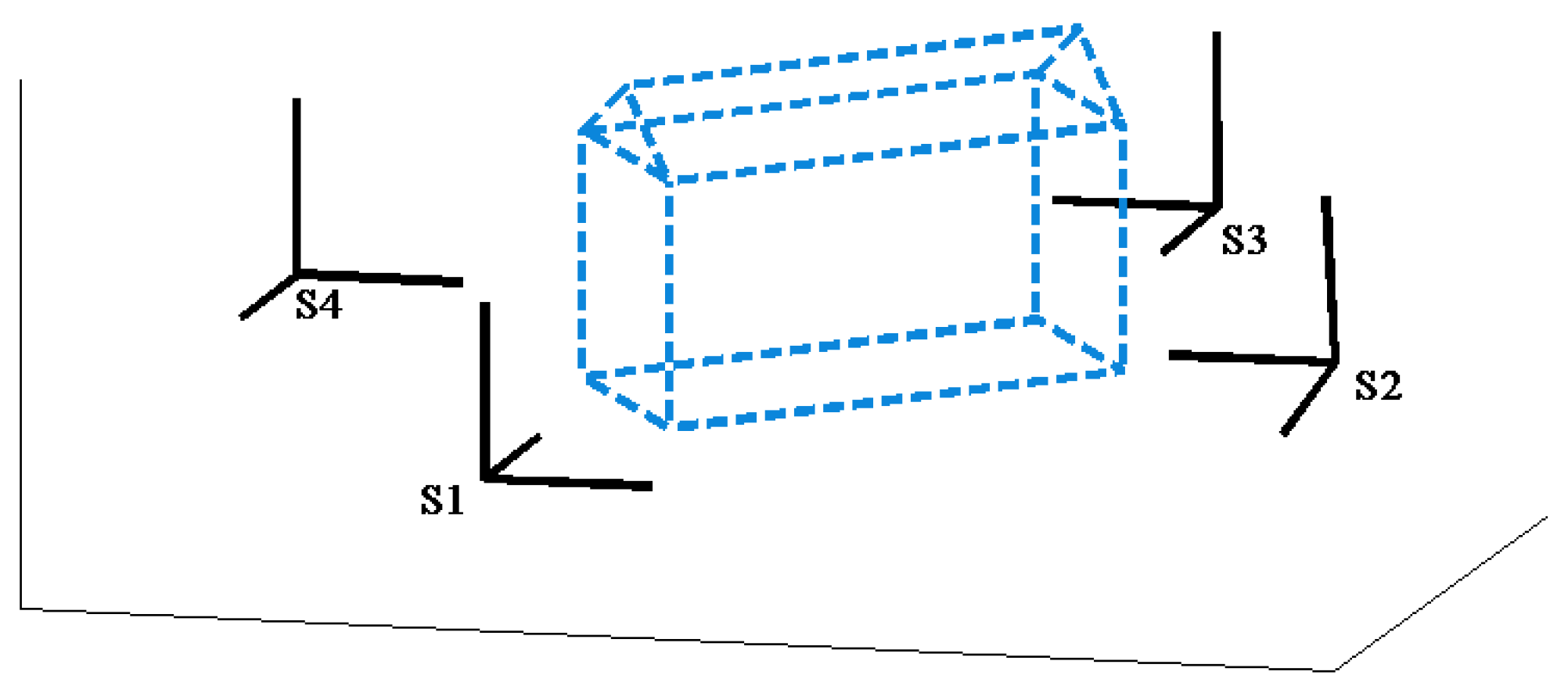
3. The Optimal Statistical Transformation Model Taking into Account Errors in Coordinate Systems

This method can be added as an appendix to any registration algorithm presented in Section 2. The registration algorithm will provide data on the found identical points, from which the transformation parameters and their covariance matrices are subsequently estimated in the regression model.

The statistical model consisting of two scans has been studied in ref. [29], under the assumption that stochastic coordinates are given only at the second coordinate system and the points of the first scan are error-less.

A more complex problem with 3D transformation arises when measurement errors are respected in both coordinate systems. Further, the following notation is used.

${\mathbf{Y}}_i$…$3(n_i+n_{i+1})$-dimensional random vector of realizations, which are obtained by the data in the i-th position of the laser sensor, $i=1,2,3,4$ (in the following text four device positions will be considered), $n_i$… number of points P in the i-th laser sensor position; (if $i=4$, then instead of $i+1$ is the number 1).

The i-th device position must be chosen so that the i-th and $(i+1)$-th measured object side must be covered by measurement. The often arbitrary i-th position may be selected as the basis for the coordinate transformation into a chosen system of coordinates.

If the chosen coordinate system is equivalent to the first cloud system then the expected value of vector ${\mathbf{Y}}_1$ is

$$\begin{array}{c}\hfill E\left({\mathbf{Y}}_1\right)=\left(\begin{array}{c}{\mathbf{fi}}_1\\ {\mathbf{\beta }}_2\end{array}\right),{\mathbf{\beta }}_1={\left({\mathbf{\beta }}_{1,1}^{\prime },\dots ,{\mathbf{\beta }}_{1,n_1}^{\prime }\right)}^{\prime },\\ \hfill {\mathbf{\beta }}_2={\left({\mathbf{\beta }}_{2,1}^{\prime },\dots ,{\mathbf{\beta }}_{2,n_2}^{\prime }\right)}^{\prime },\end{array}$$

(10)

where ${\mathbf{\beta }}_{1,j}$ are three-dimensional coordinates of the j-th point P on the first side of the object and ${\mathbf{\beta }}_{2,j}$ are three-dimensional coordinates of the j-th point on the other side of the object. If $i\ne 1$, then

$$\begin{array}{c}\hfill E\left({\mathbf{Y}}_i\right)=\left(\begin{array}{c}{\mathbf{\alpha }}_i\\ {\mathbf{\alpha }}_{i+1}\end{array}\right),\end{array}$$

(11)

where instead of $i+1$ for $i=4$ is the number 1.

$3n_i$-dimensional vector ${\mathbf{\alpha }}_i$ includes the coordinates of $n_i$ points on the i-th object side at the i-th device coordinate system. Similarly, ${\mathbf{\alpha }}_{i+1}$ has a length $3n_{i+1}$ when this vector includes the coordinates of $n_{i+1}$ points on $(i+1)$-th object side at i-th device coordinate system. It can be considered

$$\begin{array}{ccc}\hfill {\mathbf{\alpha }}_i& =& 1_{n_i}\otimes {\mathbf{\gamma }}_i+\left({\mathbf{I}}_{n_i,n_i}\otimes {\mathbf{T}}_i\right){\mathbf{\beta }}_i,\hfill \end{array}$$

(12)

$$\begin{array}{ccc}\hfill {\mathbf{\alpha }}_{i+1}& =& 1_{n_{i+1}}\otimes {\mathbf{\gamma }}_i+\left({\mathbf{I}}_{n_{i+1},n_{i+1}}\otimes {\mathbf{T}}_i\right){\mathbf{\beta }}_{i+1},\hfill \end{array}$$

(13)

where ${\mathbf{\beta }}_i$, ${\mathbf{\beta }}_{i+1}$ are vectors of point coordinates on i-th side or $(i+1)$-th object side respectively. The 3D-vector ${\mathbf{\gamma }}_i$ and the orthogonal matrix ${\mathbf{T}}_i$ are unknown and must be appropriately estimated.

Therefore

$$\begin{array}{ccc}\hfill E\left({\mathbf{Y}}_i\right)& =& \left(\begin{array}{c}{1}_{n_i}\otimes {\mathbf{\gamma }}_i\\ 1_{n_{i+1}}\otimes {\mathbf{\gamma }}_i\end{array}\right)+\hfill \\ & & \left({\mathbf{I}}_{n_i+n_{i+1},n_i+n_{i+1}}\otimes {\mathbf{T}}_i\right)\left(\begin{array}{c}{\mathbf{\beta }}_i\\ {\mathbf{\beta }}_{i+1}\end{array}\right).\hfill \end{array}$$

(14)

Further

$$\begin{array}{c}\hfill {\mathbf{T}}_i=\left(\begin{array}{ccc}{T}_{i,11},& T_{i,12},& T_{i,13}\\ T_{i,21},& T_{i,22},& T_{i,23}\\ T_{i,31},& T_{i,32},& T_{i,33}\end{array}\right),\\ \hfill {\mathbf{T}}_{i,j}=\left(\begin{array}{c}{T}_{i,1j}\\ T_{i,2j}\\ T_{i,3j}\end{array}\right),i,j=1,2,3.\end{array}$$

(15)

For simplicity, the situation will be discussed further on the model with 4 scans.

3.1. Model with Four Scans

The model with four scans is described as follows

$$E\left(\begin{array}{c}{\mathbf{Y}}_1\\ {\mathbf{Y}}_2\\ {\mathbf{Y}}_3\\ {\mathbf{Y}}_4\end{array}\right)\sim \left[\left(\begin{array}{c}{\mathbf{\beta }}_1\\ {\mathbf{\beta }}_2\\ {\mathbf{\alpha }}_2^{\left(2\right)}\\ {\mathbf{\alpha }}_3^{\left(2\right)}\\ {\mathbf{\alpha }}_3^{\left(3\right)}\\ {\mathbf{\alpha }}_4^{\left(3\right)}\\ {\mathbf{\alpha }}_4^{\left(4\right)}\\ {\mathbf{\alpha }}_1^{\left(4\right)}\end{array}\right),\mathsf{\Sigma }\right],$$

(16)

$$\begin{array}{ccc}\hfill \mathsf{\Sigma }& =& \left(\begin{array}{cccc}{\mathsf{\Sigma }}_1,& \mathbf{0},& \mathbf{0},& \mathbf{0}\\ \mathbf{0},& {\mathsf{\Sigma }}_2,& \mathbf{0},& \mathbf{0}\\ \mathbf{0},& \mathbf{0}& {\mathsf{\Sigma }}_3,& \mathbf{0}\\ \mathbf{0},& \mathbf{0}& \mathbf{0},& {\mathsf{\Sigma }}_4\end{array}\right)\hfill \end{array}$$

(17)

and constraints (for $s=2,3,4$) are

$$\begin{array}{c}\hfill {{\mathbf{T}}^{\prime }}_{s,1}{\mathbf{T}}_{s,1}=1,{{\mathbf{T}}^{\prime }}_{s,1}{\mathbf{T}}_{s,2}=0,{{\mathbf{T}}^{\prime }}_{s,1}{\mathbf{T}}_{s,3}=0,\\ \hfill {{\mathbf{T}}^{\prime }}_{s,2}{\mathbf{T}}_{s,2}=1,{{\mathbf{T}}^{\prime }}_{s,2}{\mathbf{T}}_{s,3}=0,{{\mathbf{T}}^{\prime }}_{s,3}{\mathbf{T}}_{s,3}=1,\end{array}$$

(18)

and

$$\begin{array}{ccc}\hfill {\mathbf{\alpha }}_2^{\left(2\right)}-1_{n_2}\otimes {\mathbf{\gamma }}_2-\left({\mathbf{I}}_{n_2,n_2}\otimes {\mathbf{T}}_2\right){\mathbf{\beta }}_2& =& \mathbf{0},\hfill \\ \hfill {\mathbf{\alpha }}_3^{\left(2\right)}-1_{n_3}\otimes {\mathbf{\gamma }}_2-\left({\mathbf{I}}_{n_3,n_3}\otimes {\mathbf{T}}_2\right){\mathbf{\beta }}_3& =& \mathbf{0},\hfill \\ \hfill {\mathbf{\alpha }}_3^{\left(3\right)}-1_{n_3}\otimes {\mathbf{\gamma }}_3-\left({\mathbf{I}}_{n_3,n_3}\otimes {\mathbf{T}}_3\right){\mathbf{\beta }}_3& =& \mathbf{0},\hfill \\ \hfill {\mathbf{\alpha }}_4^{\left(3\right)}-1_{n_4}\otimes {\mathbf{\gamma }}_3-\left({\mathbf{I}}_{n_4,n_4}\otimes {\mathbf{T}}_3\right){\mathbf{\beta }}_4& =& \mathbf{0},\hfill \\ \hfill {\mathbf{\alpha }}_4^{\left(4\right)}-1_{n_4}\otimes {\mathbf{\gamma }}_4-\left({\mathbf{I}}_{n_4,n_4}\otimes {\mathbf{T}}_4\right){\mathbf{\beta }}_4& =& \mathbf{0},\hfill \\ \hfill {\mathbf{\alpha }}_1^{\left(4\right)}-1_{n_1}\otimes {\mathbf{\gamma }}_4-\left({\mathbf{I}}_{n_1,n_1}\otimes {\mathbf{T}}_4\right){\mathbf{\beta }}_1& =& \mathbf{0},\hfill \end{array}$$

(19)

(${\mathbf{\alpha }}_{i+1}^{\left(i\right)}$ comprise measured coordinates on the $(i+1)$-th side of object at the i-th device coordinate system).

Unknown parameters are the following vectors

$$\begin{array}{c}\hfill {\mathbf{\beta }}_1,{\mathbf{\beta }}_2,{\mathbf{\beta }}_3,{\mathbf{\beta }}_4,{\mathbf{\alpha }}_2^{\left(2\right)},{\mathbf{\alpha }}_3^{\left(2\right)},{\mathbf{\alpha }}_3^{\left(3\right)},{\mathbf{\alpha }}_4^{\left(3\right)},{\mathbf{\alpha }}_4^{\left(4\right)},{\mathbf{\alpha }}_1^{\left(4\right)},\\ \hfill {\mathbf{\gamma }}_2,{\mathbf{\gamma }}_3,{\mathbf{\gamma }}_4,{\mathbf{T}}_{i,1},{\mathbf{T}}_{i,2},{\mathbf{T}}_{i,3},i=2,3,4.\end{array}$$

The unknown parameter count in the model is $3(n_1+n_2+n_3+n_4)+6(n_3+n_4)+3(n_1+n_2)+9+27$, and the number of constraints is $3n_1+6(n_3+n_4)+3n_2+18$. The measurements count plus constraints minus parameters is $3n-18$.

3.2. Linearization of a Model with 4 Scans

Now the linearized model will be described.

The following notation and terminology will be used:

$$\begin{array}{ccc}{\mathsf{\Theta }}_1\hfill & =\hfill & \left({\mathbf{\beta }}_1^{\prime },{\mathbf{\beta }}_2^{\prime },{\left({\mathbf{\alpha }}_2^{\left(2\right)}\right)}^{\prime },{\left({\mathbf{\alpha }}_3^{\left(2\right)}\right)}^{\prime },{\left({\mathbf{\alpha }}_3^{\left(3\right)}\right)}^{\prime },{\left({\mathbf{\alpha }}_4^{\left(3\right)}\right)}^{\prime },\right.\hfill \\ \hfill & \hfill & {\left.{\left({\mathbf{\alpha }}_4^{\left(4\right)}\right)}^{\prime },{\left({\mathbf{\alpha }}_1^{\left(4\right)}\right)}^{\prime }\right)}^{\prime },\hfill \end{array}$$

(20)

$$\begin{array}{ccc}{\mathsf{\Theta }}_2\hfill & =\hfill & \left({\mathbf{\beta }}_3^{\prime },{\mathbf{\beta }}_4^{\prime },{\mathbf{\gamma }}_2^{\prime },{\mathbf{\gamma }}_3^{\prime },{\mathbf{\gamma }}_4^{\prime },{\left[\mathrm{vec}\left({\mathbf{T}}_2\right)\right]}^{\prime },\right.\hfill \\ \hfill & \hfill & {\left.{\left[\mathrm{vec}\left({\mathbf{T}}_3\right)\right]}^{\prime },{\left[\mathrm{vec}\left({\mathbf{T}}_4\right)\right]}^{\prime }\right)}^{\prime },\hfill \end{array}$$

(21)

$$\begin{array}{ccc}\hfill \mathbf{Y}& =& \left({\mathbf{Y}}_1^{\prime },{\mathbf{Y}}_2^{\prime },{\mathbf{Y}}_3^{\prime },{\mathbf{Y}}_4^{\prime }\right),\hfill \end{array}$$

(22)

$$\begin{array}{ccc}\hfill \mathsf{\Sigma }& =& \left({\mathsf{\Sigma }}_1,{\mathsf{\Sigma }}_2,{\mathsf{\Sigma }}_3,{\mathsf{\Sigma }}_4\right).\hfill \end{array}$$

(23)

Let ${\mathsf{\Theta }}_1^{\left(0\right)},{\mathsf{\Theta }}_2^{\left(0\right)}$ are approximate values of parameters ${\mathsf{\Theta }}_1,{\mathsf{\Theta }}_2$.

The linear version of constraints is $\mathbf{b}+{\mathbf{B}}_1\delta {\mathsf{\Theta }}_1+{\mathbf{B}}_2\delta {\mathsf{\Theta }}_2=\mathbf{0}$, where $\delta {\mathsf{\Theta }}_1={\mathsf{\Theta }}_1-{\mathsf{\Theta }}_1^{\left(0\right)}$, $\delta {\mathsf{\Theta }}_2={\mathsf{\Theta }}_2-{\mathsf{\Theta }}_2^{\left(0\right)}$ and matrices ${\mathbf{B}}_1$ and ${\mathbf{B}}_2$ are given in

Table 3. Measurements.

Y${}_1^{\mathit{I}}$	Y${}_1^{\mathit{II}}$	Y${}_2^{\mathit{II}}$	Y${}_2^{\mathit{III}}$	Y${}_3^{\mathit{III}}$	Y${}_3^{\mathit{IV}}$	Y${}_4^{\mathit{IV}}$	Y${}_4^{\mathit{I}}$
629.1793	629.0871	521.6030	533.7651	−457.5236	−446.6342	208.9794	223.0744
84.1583	84.0498	−464.5526	−469.4856	−258.9134	−265.6701	702.7168	691.0423
15.1976	4.0980	4.0980	16.6208	26.6208	17.8997	22.8997	30.1976
626.6654	638.7188	532.2563	536.3855	−451.5327	−445.1702	209.2158	218.5299
87.9686	90.5740	−468.8736	−462.9402	−262.6306	−263.4124	700.0364	690.6115
3.5058	7.8426	7.8426	7.7437	17.7437	12.0001	17.0001	18.5058
622.4489	640.0699	533.7651	536.7300	−450.7452	−444.5112	209.3221	210.9074
94.3597	91.4826	−469.4856	−462.0798	−263.1193	−262.3962	698.8299	689.8890
4.0666	5.5998	5.5998	3.3267	13.3267	14.6452	19.6452	19.0666
622.0117			536.5612	−451.1310	−443.3154	209.5151	210.1170
95.0224			−462.5013	−262.8799	−260.5522	696.6406	689.8140
3.0727			16.2879	26.2879	17.3570	22.3570	18.0727
			538.5282	−446.6342	−445.0099	209.2416
			−457.5883	−265.6701	−263.1652	699.7429
			17.6355	27.6355	20.7081	25.7081
					−439.5869	210.1170
					−254.8022	689.8140
					14.7198	19.7198
$n_1=4$	$n_2=3$		$n_3=5$		$n_4=6$		$n_1=4$

.

3.3. The Estimates of Unknown Parameters in a Model with 4 Scans

The indirect measurement model with II type constraints is

$$\mathbf{Y}\sim (\mathbf{X}{\mathsf{\Theta }}_1,\mathsf{\Sigma }),\mathbf{b}+{\mathbf{B}}_1{\mathsf{\Theta }}_1+{\mathbf{B}}_2{\mathsf{\Theta }}_1=\mathbf{0}.$$

If rank $\left({\mathbf{X}}_{n,k}\right)=k_1<n,$ rank $({\mathbf{B}}_{1,(q,k_1)},{\mathbf{B}}_{2,(q,k_2)})=q<k_1+k_2,$ rank $\left({\mathbf{B}}_2\right)=k_2<q,$ and $\mathsf{\Sigma }$ is a positive definite, then the model is regular.

black of vector $\left(\begin{array}{c}{\mathsf{\Theta }}_1\\ {\mathsf{\Theta }}_1\end{array}\right)$ is given by formula

$$\begin{array}{ccc}\left(\begin{array}{c}{\widehat{\widehat{\mathsf{\Theta }}}}_1\\ {\widehat{\widehat{\mathsf{\Theta }}}}_2\end{array}\right)\hfill & =\hfill & -\left(\begin{array}{c}{\left({\mathbf{X}}^{\prime }{\mathsf{\Sigma }}^{-1}\mathbf{X}\right)}^{-1}{\mathbf{B}}_1^{\prime }{\mathbf{Q}}_{1,1}\\ {\mathbf{Q}}_{2,1}\end{array}\right)\mathbf{b}+\hfill \\ \hfill & \hfill & +\left(\begin{array}{c}\mathbf{I}-{\left({\mathbf{X}}^{\prime }{\mathsf{\Sigma }}^{-1}\mathbf{X}\right)}^{-1}{\mathbf{B}}_1^{\prime }{\mathbf{Q}}_{1,1}{\mathbf{B}}_1\\ -{\mathbf{Q}}_{2,1}{\mathbf{B}}_1\end{array}\right){\widehat{\mathsf{\Theta }}}_1,\hfill \end{array}$$

(24)

where ${\widehat{\mathsf{\Theta }}}_1={\left({\mathbf{X}}^{\prime }{\mathsf{\Sigma }}^{-1}\mathbf{X}\right)}^{-1}{\mathbf{X}}^{\prime }{\mathsf{\Sigma }}^{-1}\mathbf{Y}$ (estimate non-respecting the parameters ${\mathsf{\Theta }}_1,{\mathsf{\Theta }}_2$ constraints); covariance matrix is

$$\begin{array}{cc}& \mathrm{var}\left(\begin{array}{c}{\widehat{\widehat{\mathsf{\Theta }}}}_1\\ {\widehat{\widehat{\mathsf{\Theta }}}}_2\end{array}\right)=\left(\begin{array}{cc}\mathrm{var}\left({\widehat{\widehat{\mathsf{\Theta }}}}_1\right),& \mathrm{cov}({\widehat{\widehat{\mathsf{\Theta }}}}_1,{\widehat{\widehat{\mathsf{\Theta }}}}_2)\\ \mathrm{cov}({\widehat{\widehat{\mathsf{\Theta }}}}_2,{\widehat{\widehat{\mathsf{\Theta }}}}_1),& \mathrm{var}\left({\widehat{\widehat{\mathsf{\Theta }}}}_2\right)\end{array}\right),\end{array}$$

(25)

where

$$\begin{array}{ccc}\hfill \mathrm{var}\left({\widehat{\widehat{\mathsf{\Theta }}}}_1\right)& =& {\left({\mathbf{X}}^{\prime }{\mathsf{\Sigma }}^{-1}\mathbf{X}\right)}^{-1}-{\left({\mathbf{X}}^{\prime }{\mathsf{\Sigma }}^{-1}\mathbf{X}\right)}^{-1}{\mathbf{B}}_1^{\prime }\times \hfill \\ & & {\mathbf{Q}}_{1,1}{\mathbf{B}}_1{\left({\mathbf{X}}^{\prime }{\mathsf{\Sigma }}^{-1}\mathbf{X}\right)}^{-1},\hfill \end{array}$$

$$\mathrm{cov}({\widehat{\widehat{\mathsf{\Theta }}}}_1,{\widehat{\widehat{\mathsf{\Theta }}}}_2)=-{\left({\mathbf{X}}^{\prime }{\mathsf{\Sigma }}^{-1}\mathbf{X}\right)}^{-1}{\mathbf{B}}_1^{\prime }{\mathbf{Q}}_{1,2},$$

$$\mathrm{var}\left({\widehat{\widehat{\mathsf{\Theta }}}}_2\right)=-{\mathbf{Q}}_{2,2},$$

and

$$\left(\begin{array}{cc}{\mathbf{Q}}_{1,1},& {\mathbf{Q}}_{1,2}\\ {\mathbf{Q}}_{2,1},& {\mathbf{Q}}_{2,2}\end{array}\right)={\left(\begin{array}{cc}{\mathbf{B}}_1{\left({\mathbf{X}}^{\prime }{\mathsf{\Sigma }}^{-1}\mathbf{X}\right)}^{-1}{\mathbf{B}}_1^{\prime },& {\mathbf{B}}_2\\ {\mathbf{B}}_2^{\prime },& \mathbf{0}\end{array}\right)}^{-1}.$$

Proof in [30].

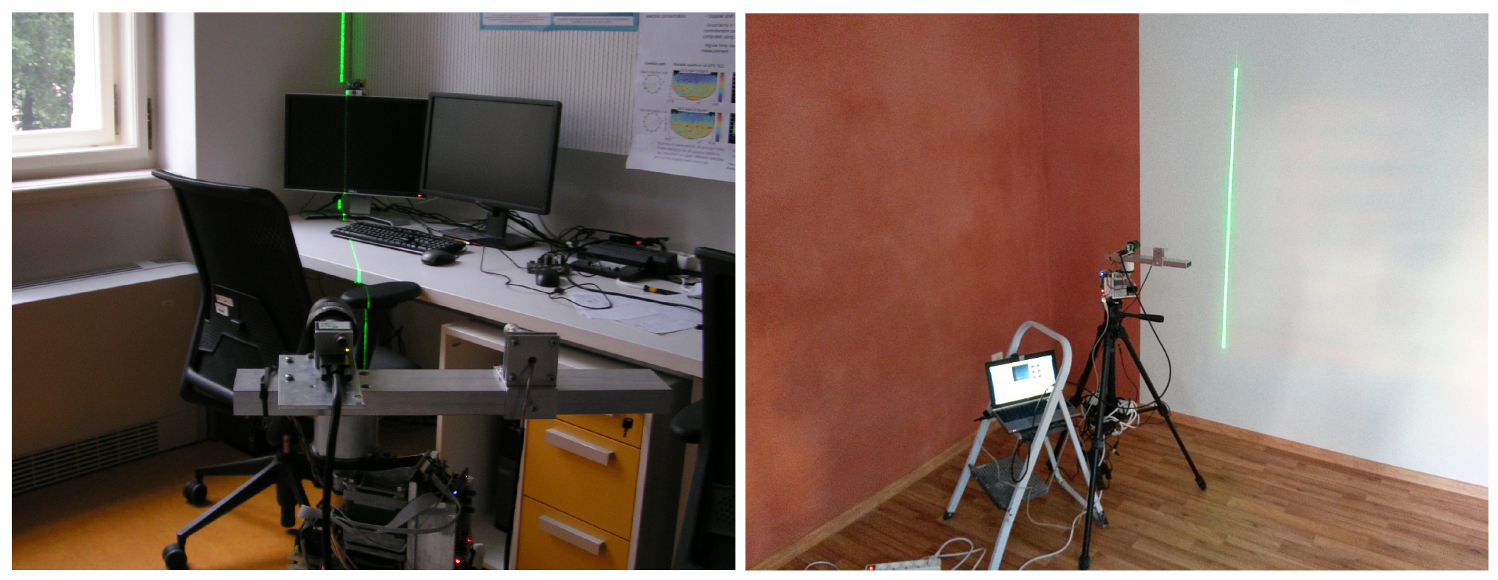
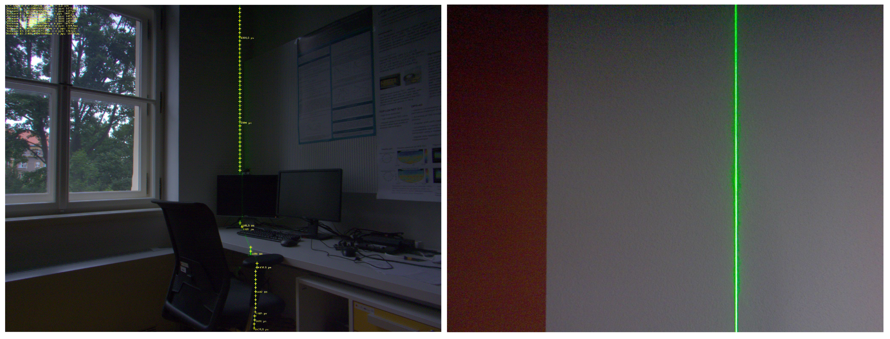
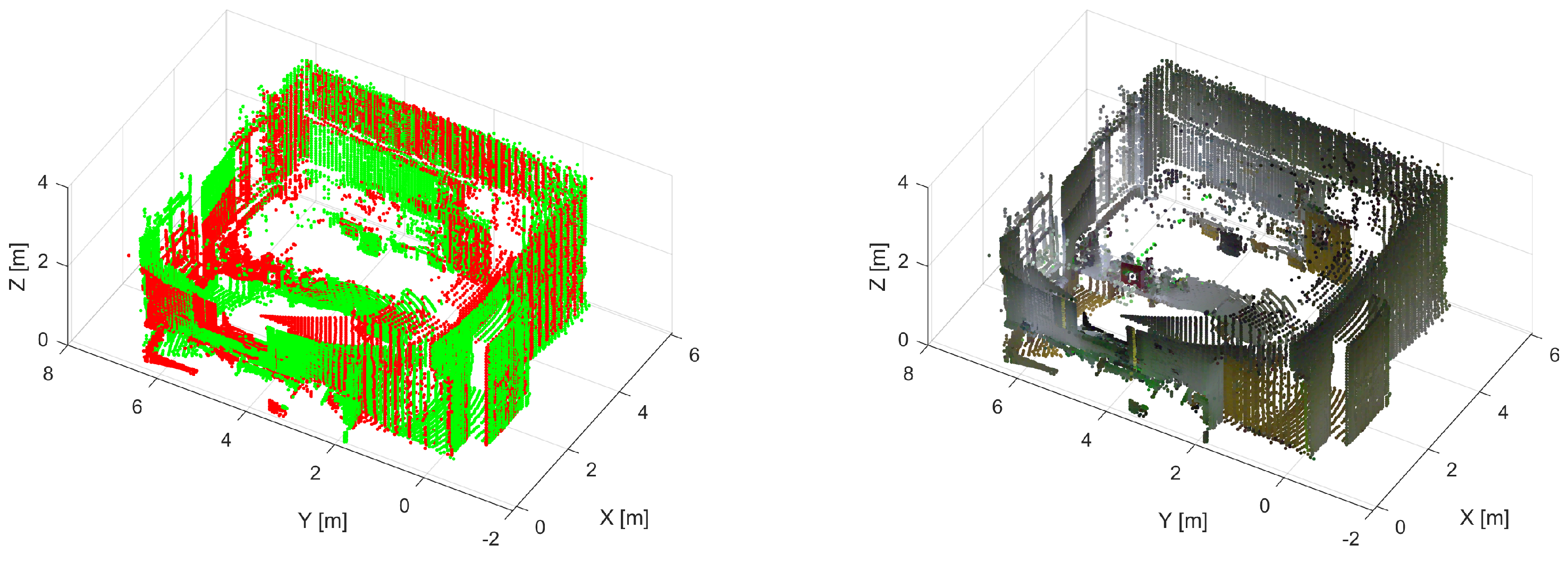
3.4. Numerical Study

In the following example, the transformation parameters will be calculated in a simulated problem. We will consider a model of a building with four scans (coordinate systems) of measurement. See Figure 5 .

Let ${\mathbf{Y}}_1=\left(\begin{array}{c}{\mathbf{Y}}_1^I\\ {\mathbf{Y}}_1^{II}\end{array}\right)$, ${\mathbf{Y}}_2=\left(\begin{array}{c}{\mathbf{Y}}_2^{II}\\ {\mathbf{Y}}_2^{III}\end{array}\right)$,

${\mathbf{Y}}_3=\left(\begin{array}{c}{\mathbf{Y}}_3^{III}\\ {\mathbf{Y}}_3^{IV}\end{array}\right)$, ${\mathbf{Y}}_4=\left(\begin{array}{c}{\mathbf{Y}}_4^{IV}\\ {\mathbf{Y}}_4^I\end{array}\right)$.

For example, ${\mathbf{Y}}_1^I$ includes the measured coordinates on the I-side of an object that are given in the first stage of measurement. Vector ${\mathbf{Y}}_1^{II}$ encompasses the measured coordinates on the II-side of an object that are given in the second stage of measurement.

Figure 5. Layout of measurement with 4 scans.

Figure 5. Layout of measurement with 4 scans.

In Table 3, we present the measured coordinates:

We assume the coordinate accuracy of measured points in all scans to be approximately the same and to be given by a standard deviation of 10 mm.

For the above-mentioned algorithm, estimators of unknown parameters of translation and rotation will be calculated. During linearization, matrices obtained from partial derivations of the model according to individual parameters are used. The calculated matrices are given in Appendix A,

Table A1. Matrices ${\mathbf{B}}_1$ and ${\mathbf{B}}_2$.

${\left\{{\mathbf{B}}_1\right\}}_{\mathbf{i}=1}^{3{\mathit{n}}_2}=$	$\frac{\partial }{\partial {\mathsf{\Theta }}_1^{\prime }}{\left[{\mathit{\alpha }}_2^{\left(2\right)}\mathbf{-}{\mathbf{1}}_{n_2}\otimes {\mathit{\gamma }}_2-\left({\mathbf{I}}_{n_2}\otimes {\mathbf{T}}_2\right){\mathit{\beta }}_2\right]}_{{\mathsf{\Theta }}_1={\mathsf{\Theta }}_1^{\left(0\right)},{\mathsf{\Theta }}_2={\mathsf{\Theta }}_2^{\left(0\right)}}=$	$\left({\mathbf{0}}_{3n_2,3n_1},-({\mathbf{I}}_{n_2}\otimes {\mathbf{T}}_2^{\left(0\right)}),{\mathbf{I}}_{3n_2},{\mathbf{0}}_{3n_2,3n_3},{\mathbf{0}}_{3n_2,3n_3},{\mathbf{0}}_{3n_2,3n_4},{\mathbf{0}}_{3n_2,3n_4},{\mathbf{0}}_{3n_2,3n_1}\right),$
${\left\{{\mathbf{B}}_1\right\}}_{i=3n_2+1}^{3n_2+3n_3}=$	$\frac{\partial }{\partial {\mathsf{\Theta }}_1^{\prime }}{\left[{\mathbf{\alpha }}_3^{\left(2\right)}\mathbf{-}{\mathbf{1}}_{n_3}\otimes {\mathbf{\gamma }}_2-\left({\mathbf{I}}_{n_3}\otimes {\mathbf{T}}_2\right){\mathbf{\beta }}_3\right]}_{{\mathsf{\Theta }}_1={\mathsf{\Theta }}_1^{\left(0\right)},{\mathsf{\Theta }}_2={\mathsf{\Theta }}_2^{\left(0\right)}}=$	$\left({\mathbf{0}}_{3n_3,3n_1},{\mathbf{0}}_{3n_3,3n_2},{\mathbf{0}}_{3n_3,3n_2},{\mathbf{I}}_{3n_3},{\mathbf{0}}_{3n_3,3n_3},{\mathbf{0}}_{3n_3,3n_4},{\mathbf{0}}_{3n_3,3n_4},{\mathbf{0}}_{3n_3,3n_1}\right),$
${\left\{{\mathbf{B}}_1\right\}}_{i=3n_2+3n_3+1}^{3n_2+3n_3+3n_3}=$	$\frac{\partial }{\partial {\mathsf{\Theta }}_1^{\prime }}{\left[{\mathbf{\alpha }}_3^{\left(3\right)}\mathbf{-}{\mathbf{1}}_{n_3}\otimes {\mathbf{\gamma }}_3-\left({\mathbf{I}}_{n_3}\otimes {\mathbf{T}}_3\right){\mathbf{\beta }}_3\right]}_{{\mathsf{\Theta }}_1={\mathsf{\Theta }}_1^{\left(0\right)},{\mathsf{\Theta }}_2={\mathsf{\Theta }}_2^{\left(0\right)}}=$	$\left({\mathbf{0}}_{3n_3,3n_1},{\mathbf{0}}_{3n_3,3n_2},{\mathbf{0}}_{3n_3,3n_2},{\mathbf{0}}_{3n_3,3n_3},{\mathbf{I}}_{3n_3},{\mathbf{0}}_{3n_3,3n_4},{\mathbf{0}}_{3n_3,3n_4},{\mathbf{0}}_{3n_3,3n_1}\right),$
${\left\{{\mathbf{B}}_1\right\}}_{i=3n_2+6n_3+1}^{3n_2+6n_3+3n_4}=$	$\frac{\partial }{\partial {\mathsf{\Theta }}_1^{\prime }}{\left[{\mathbf{\alpha }}_4^{\left(3\right)}\mathbf{-}{\mathbf{1}}_{n_4}\otimes {\mathbf{\gamma }}_3-\left({\mathbf{I}}_{n_4}\otimes {\mathbf{T}}_3\right){\mathbf{\beta }}_4\right]}_{{\mathsf{\Theta }}_1={\mathsf{\Theta }}_1^{\left(0\right)},{\mathsf{\Theta }}_2={\mathsf{\Theta }}_2^{\left(0\right)}}=$	$\left({\mathbf{0}}_{3n_4,3n_1},{\mathbf{0}}_{3n_4,3n_2},{\mathbf{0}}_{3n_4,3n_2},{\mathbf{0}}_{3n_4,3n_3},{\mathbf{0}}_{3n_4,3n_3},{\mathbf{I}}_{3n_4},{\mathbf{0}}_{3n_4,3n_4},{\mathbf{0}}_{3n_4,3n_1}\right),$
${\left\{{\mathbf{B}}_1\right\}}_{i=3n_2+6n_3+3n_4+1}^{3n_2+6n_3+6n_4}=$	$\frac{\partial }{\partial {\mathsf{\Theta }}_1^{\prime }}{\left[{\mathbf{\alpha }}_4^{\left(4\right)}\mathbf{-}{\mathbf{1}}_{n_4}\otimes {\mathbf{\gamma }}_4-\left({\mathbf{I}}_{n_4}\otimes {\mathbf{T}}_4\right){\mathbf{\beta }}_4\right]}_{{\mathsf{\Theta }}_1={\mathsf{\Theta }}_1^{\left(0\right)},{\mathsf{\Theta }}_2={\mathsf{\Theta }}_2^{\left(0\right)}}=$	$\left({\mathbf{0}}_{3n_4,3n_1},{\mathbf{0}}_{3n_4,3n_2},{\mathbf{0}}_{3n_4,3n_2},{\mathbf{0}}_{3n_4,3n_3},{\mathbf{0}}_{3n_4,3n_3},{\mathbf{0}}_{3n_4,3n_4},{\mathbf{I}}_{3n_4},{\mathbf{0}}_{3n_4,3n_1}\right),$
${\left\{{\mathbf{B}}_1\right\}}_{i=3n_2+6n_3+6n_4+1}^{3n_2+6n_3+6n_4+3n_1}=$	$\frac{\partial }{\partial {\mathsf{\Theta }}_1^{\prime }}{\left[{\mathbf{\alpha }}_1^{\left(4\right)}\mathbf{-}{\mathbf{1}}_{n_1}\otimes {\mathbf{\gamma }}_4-\left({\mathbf{I}}_{n_1}\otimes {\mathbf{T}}_4\right){\mathbf{\beta }}_1\right]}_{{\mathsf{\Theta }}_1={\mathsf{\Theta }}_1^{\left(0\right)},{\mathsf{\Theta }}_2={\mathsf{\Theta }}_2^{\left(0\right)}}=$	$\left(-\left({\mathbf{I}}_{n_1}\otimes {\mathbf{T}}_4\right),{\mathbf{0}}_{3n_1,3n_2},{\mathbf{0}}_{3n_1,3n_2},{\mathbf{0}}_{3n_1,3n_3},{\mathbf{0}}_{3n_1,3n_3},{\mathbf{0}}_{3n_1,3n_4},{\mathbf{0}}_{3n_1,3n_4},{\mathbf{I}}_{3n_1}\right),$
${\left\{{\mathbf{B}}_1\right\}}_{i=3n_1+3n_2+6n_3+6n_4+1}^{3(n_1+n_2)+6(n_3+n_4)+18}=$		${\mathbf{0}}_{18,6(n_1+n_2+n_3+n_4)}.$
${\left\{{\mathbf{B}}_2\right\}}_{i=1}^{3n_2}=$	$\frac{\partial }{\partial {\mathsf{\Theta }}_2^{\prime }}{\left[{\mathbf{\alpha }}_2^{\left(2\right)}\mathbf{-}{\mathbf{1}}_{n_2}\otimes {\mathbf{\gamma }}_2-\left({\mathbf{I}}_{n_2}\otimes {\mathbf{T}}_2\right){\mathbf{\beta }}_2\right]}_{{\mathsf{\Theta }}_1={\mathsf{\Theta }}_1^{\left(0\right)},{\mathsf{\Theta }}_2={\mathsf{\Theta }}_2^{\left(0\right)}}=$	$\left({\mathbf{0}}_{3n_2,3n_3},{\mathbf{0}}_{3n_2,3n_4},-1_{n_2}\otimes {\mathbf{I}}_3,{\mathbf{0}}_{3n_2,3},{\mathbf{0}}_{3n_2,3},-{\mathbf{\beta }}_2^{\prime }\otimes {\mathbf{I}}_{n_3},{\mathbf{0}}_{3n_2,9},{\mathbf{0}}_{3n_2,9}\right),$
${\left\{{\mathbf{B}}_2\right\}}_{i=3n_2+1}^{3n_2+3n_3}=$	$\frac{\partial }{\partial {\mathsf{\Theta }}_2^{\prime }}{\left[{\mathbf{\alpha }}_3^{\left(2\right)}\mathbf{-}{\mathbf{1}}_{n_3}\otimes {\mathbf{\gamma }}_2-\left({\mathbf{I}}_{n_3}\otimes {\mathbf{T}}_2\right){\mathbf{\beta }}_3\right]}_{{\mathsf{\Theta }}_1={\mathsf{\Theta }}_1^{\left(0\right)},{\mathsf{\Theta }}_2={\mathsf{\Theta }}_2^{\left(0\right)}}=$	$\left((-{\mathbf{I}}_{n_3}\otimes {\mathbf{T}}_2),{\mathbf{0}}_{3n_3,3n_4},{\mathbf{0}}_{3n_3,3},-1_{n_3}\otimes {\mathbf{I}}_3,{\mathbf{0}}_{3n_3,3},-{\mathbf{\beta }}_3^{\prime }\otimes {\mathbf{I}}_{n_3},{\mathbf{0}}_{3n_3,9},{\mathbf{0}}_{3n_3,9}\right),$
${\left\{{\mathbf{B}}_2\right\}}_{i=3n_2+3n_3+1}^{3n_2+6n_3}=$	$\frac{\partial }{\partial {\mathsf{\Theta }}_2^{\prime }}{\left[{\mathbf{\alpha }}_3^{\left(3\right)}\mathbf{-}{\mathbf{1}}_{n_3}\otimes {\mathbf{\gamma }}_3-\left({\mathbf{I}}_{n_3}\otimes {\mathbf{T}}_3\right){\mathbf{\beta }}_3\right]}_{{\mathsf{\Theta }}_1={\mathsf{\Theta }}_1^{\left(0\right)},{\mathsf{\Theta }}_2={\mathsf{\Theta }}_2^{\left(0\right)}}=$	$\left((-{\mathbf{I}}_{n_3}\otimes {\mathbf{T}}_3),{\mathbf{0}}_{3n_3,3n_4},{\mathbf{0}}_{3n_3,3},-1_{n_3}\otimes {\mathbf{I}}_3,{\mathbf{0}}_{3n_3,3},{\mathbf{0}}_{3n_3,9},-{\mathbf{\beta }}_3^{\prime }\otimes {\mathbf{I}}_{n_3},{\mathbf{0}}_{3n_3,9}\right),$
${\left\{{\mathbf{B}}_2\right\}}_{i=3n_2+6n_3+1}^{3n_2+6n_3+3n_4}=$	$\frac{\partial }{\partial {\mathsf{\Theta }}_2^{\prime }}{\left[{\mathbf{\alpha }}_4^{\left(3\right)}\mathbf{-}{\mathbf{1}}_{n_4}\otimes {\mathbf{\gamma }}_3-\left({\mathbf{I}}_{n_4}\otimes {\mathbf{T}}_3\right){\mathbf{\beta }}_4\right]}_{{\mathsf{\Theta }}_1={\mathsf{\Theta }}_1^{\left(0\right)},{\mathsf{\Theta }}_2={\mathsf{\Theta }}_2^{\left(0\right)}}=$	$\left({\mathbf{0}}_{3n_4,3n_3},(-{\mathbf{I}}_{n_4}\otimes {\mathbf{T}}_3),{\mathbf{0}}_{3n_4,3},-1_{n_4}\otimes {\mathbf{I}}_3,{\mathbf{0}}_{3n_4,3},{\mathbf{0}}_{3n_4,9},-{\mathbf{\beta }}_4^{\prime }\otimes {\mathbf{I}}_{n_3},{\mathbf{0}}_{3n_4,9}\right),$
${\left\{{\mathbf{B}}_2\right\}}_{i=3n_2+6n_3+3n_4+1}^{3n_2+6n_3+6n_4}=$	$\frac{\partial }{\partial {\mathsf{\Theta }}_2^{\prime }}{\left[{\mathbf{\alpha }}_4^{\left(4\right)}\mathbf{-}{\mathbf{1}}_{n_4}\otimes {\mathbf{\gamma }}_4-\left({\mathbf{I}}_{n_4}\otimes {\mathbf{T}}_4\right){\mathbf{\beta }}_4\right]}_{{\mathsf{\Theta }}_1={\mathsf{\Theta }}_1^{\left(0\right)},{\mathsf{\Theta }}_2={\mathsf{\Theta }}_2^{\left(0\right)}}=$	$\left({\mathbf{0}}_{3n_4,3n_3},(-{\mathbf{I}}_{n_4}\otimes {\mathbf{T}}_4),{\mathbf{0}}_{3n_4,3},{\mathbf{0}}_{3n_4,3},-1_{n_4}\otimes {\mathbf{I}}_3,{\mathbf{0}}_{3n_4,9},{\mathbf{0}}_{3n_4,9},-{\mathbf{\beta }}_4^{\prime }\otimes {\mathbf{I}}_{n_3}\right),$
${\left\{{\mathbf{B}}_2\right\}}_{i=3n_2+6(n_3+n_4)+1}^{3n_2+6(n_3+n_4)+3n_1}=$	$\frac{\partial }{\partial {\mathsf{\Theta }}_2^{\prime }}{\left[{\mathbf{\alpha }}_1^{\left(4\right)}\mathbf{-}{\mathbf{1}}_{n_1}\otimes {\mathbf{\gamma }}_4-\left({\mathbf{I}}_{n_1}\otimes {\mathbf{T}}_4\right){\mathbf{\beta }}_1\right]}_{{\mathsf{\Theta }}_1={\mathsf{\Theta }}_1^{\left(0\right)},{\mathsf{\Theta }}_2={\mathsf{\Theta }}_2^{\left(0\right)}}=$	$\left({\mathbf{0}}_{3n_1,3n_3},{\mathbf{0}}_{3n_1,3n_4},{\mathbf{0}}_{3n_1,3},{\mathbf{0}}_{3n_1,3},-1_{n_1}\otimes {\mathbf{I}}_3,{\mathbf{0}}_{3n_1,9},{\mathbf{0}}_{3n_1,9},-{\mathbf{\beta }}_1^{\prime }\otimes {\mathbf{I}}_3\right)$  .

.

Estimates computed by Formula (24) are

$$\begin{array}{ccc}\hfill {\widehat{\mathbf{T}}}_2& =& \left(\begin{array}{ccc}0.55919& 0.82904& 0\\ -0.82904& 0.55919& 0\\ 0& 0& 0\end{array}\right),\hfill \\ \hfill {\widehat{\mathbf{T}}}_3& =& \left(\begin{array}{ccc}-0.91355& 0.40674& 0\\ -0.40674& -0.91355& 0\\ 0& 0& 0\end{array}\right),\hfill \\ \hfill {\widehat{\mathbf{T}}}_4& =& \left(\begin{array}{ccc}0.46947& -0.88295& 0\\ 0.88295& 0.46947& 0\\ 0& 0& 0\end{array}\right),\hfill \\ \hfill {\widehat{\mathbf{\gamma }}}_2& =& {(99.3732,10.8637,0.0000)}^{\prime },\hfill \\ \hfill {\widehat{\mathbf{\gamma }}}_3& =& {(89.6260,84.0564,9.9873)}^{\prime },\hfill \\ \hfill {\widehat{\mathbf{\gamma }}}_4& =& {(2.5764,95.9541,15.0178)}^{\prime }.\hfill \end{array}$$

Furthermore, the resulting estimators of coordinates obtained in the system of scan 1 and absolute point positioning errors obtained from (25) are shown in

Table 4. Estimates of coordinates.

${\widehat{\mathsf{\beta }}}_1$	${}^{\mathit{s}}$${\widehat{\mathsf{\beta }}}_1$	${\widehat{\mathsf{\beta }}}_2$	${}^{\mathit{s}}$${\widehat{\mathsf{\beta }}}_2$	${\widehat{\mathsf{\beta }}}_3$	${}^{\mathit{s}}$${\widehat{\mathsf{\beta }}}_3$	${\widehat{\mathsf{\beta }}}_4$	${}^{\mathit{s}}$${\widehat{\mathsf{\beta }}}_4$
629.2236	0.0134	629.2727	0.0151	639.9965	0.0254	632.7031	0.1205
84.0842	0.0162	84.1765	0.0108	91.4590	0.0235	102.1926	0.1057
14.8946	0.0180	4.2584	0.0149	16.7208	0.0232	7.9921	0.1125
626.7046	0.0121	638.7539	0.0133	636.1058	0.0753	630.6615	0.0852
87.9179	0.0107	90.4175	0.0154	97.5176	0.0541	100.7179	0.0816
3.4601	0.0155	7.8524	0.0151	7.5773	0.0429	2.0002	0.0344
622.3238	0.0142	640.0670	0.0180	635.6114	0.0907	629.4778	0.0233
94.3276	0.0139	91.4741	0.0189	97.8561	0.0687	99.8918	0.0422
4.1908	0.0188	5.6040	0.0201	3.2677	0.0789	4.6397	0.0179
621.9169	0.0190			635.8859	0.0595	627.7632	0.0912
95.0236	0.0224			97.9292	0.0614	98.7844	0.0894
2.9661	0.0256			16.2601	0.0209	7.4481	0.0796
				632.8328	0.1003	630.4326	0.0488
				102.1181	0.0982	100.3622	0.0198
				17.6777	0.1143	10.7676	0.0158
						622.0444	0.0129
						94.8902	0.0164
						4.7548	0.0246

.

4. Concluding Remarks

The paper attempts to present a state-of-the-art solution to the registration problem. Indeed, there are data registration problems that require high complexity for the laser systems and algorithms used. Many previously presented methods lack variability estimations. Our statistical model can serve as a complement to any registration algorithm since it provides an estimate of the variance matrix based on the knowledge of identical points. The method requires covariance matrix knowledge for identical point coordinates. The solution includes translational parameter estimation and the rotation matrix between the several coordinate systems. Unknown transformation parameters and the variance matrix were estimated by using the nonlinear regression model with nonlinear constraints. Separately, this approach is applicable in the case of geodetic measurements, when identical points are marked with reflective targets.

References

1. Goshtasby, A.A. Image Registration; Advances in Pattern Recognition; Springer: London, UK, 2012. [Google Scholar] [CrossRef]
2. Pomerleau, F.; Colas, F.; Siegwart, R. A Review of Point Cloud Registration Algorithms for Mobile Robotics. Found. Trends Robot. 2015, 4, 1–104. [Google Scholar] [CrossRef]
3. Cheng, L.; Chen, S.; Liu, X.; Xu, H.; Wu, Y.; Li, M.; Chen, Y. Registration of laser scanning point clouds: A review. Sensors. Multidisciplinary Digital Publishing Institute. Sensors 2018, 18, 1641. [Google Scholar] [CrossRef]
4. Dong, Z.; Liang, F.; Yang, B.; Xu, Y.; Zang, Y.; Li, J.; Wang, Y.; Dai, W.; Fan, H.; Hyypp, J.; et al. Registration of large-scale terrestrial laser scanner point clouds: A review and benchmark. ISPRS J. Photogramm. Remote Sens. 2020, 163, 327–342. [Google Scholar] [CrossRef]
5. Kopacik, A.; Erdeeyi, J.; Kyrinovic, P. Engineering Surveys for Industry, Chapter Terrestrial Laser Scanning Systems; Springer: Berlin/Heidelberg, Germany, 2020; ISBN 9783030483081. [Google Scholar] [CrossRef]
6. Chmelar, P.; Rejfek, L.; Nguyen, T.N.; Ha, D. Advanced Methods for Point Cloud Processing and Simplification. Appl. Sci. 2020, 10, 3340. [Google Scholar] [CrossRef]
7. Chen, Y.; Gerard, M. Object modelling by registration of multiple range images. Image Vision Comput. 1991, 10, 145–155. [Google Scholar] [CrossRef]
8. Besl, P.J.; McKay, N.D. A Method for Registration of 3-D Shapes. IEEE Trans. Pattern Anal. Mach. Intell. 1992, 14, 239–256. [Google Scholar] [CrossRef]
9. Nüchter, A. 3D Robotic Mapping: The Simultaneous Localization and Mapping Problem with Six Degrees of Freedom; Springer: Berlin/Heidelberg, Germany, 2009; ISBN 978-354089883-2. ISSN 16107438. [Google Scholar] [CrossRef]
10. Nüchter, A.; Elseberg, J.; Schneider, P.; Paulus, D. Study of parameterizations for the rigid body transformations of the scan registration problem. Comput. Vis. Image Underst. 2010, 114, 963–980. [Google Scholar] [CrossRef]
11. Peter, B.; Wolfgang, S. The normal distributions transform: A new approach to laser scan matching. In Proceedings of the 2003 IEEE/RSJ International Conference on Intelligent Robots and Systems (IROS 2003) (Cat. No. 03CH37453), Las Vegas, NV, USA, 27–31 October 2003; Volume 3, pp. 2743–2748. [Google Scholar]
12. Magnusson, M.; Lilienthal, A.; Duckett, T. Scan registration for autonomous mining vehicles using 3D-NDT. J. Field Robot. 2007, 24, 803–827. [Google Scholar] [CrossRef]
13. Magnusson, M. The Three-Dimensional Normal-Distributions Transform an Efficient Representation for Registration, Surface Analysis, and Loop Detection. In Studies in Technology; Örebro University: Örebro, Sweden, 2013. [Google Scholar]
14. Beran, L.; Chmelar, P.; Rejfek, L. Navigation of Robotics Platform Using Advanced Image Processing Navigation Methods. In Proceedings of the VIPIMAGE (V. Eccomas Thematic Conference on Computional Vision and Medical Image Processing), Tenerife, Spain, 19–21 October 2015; ISBN 978-113802926-2. [Google Scholar]
15. Beran, L.; Chmelar, P.; Rejfek, L. Navigation of Robotics Platform using Monocular Visual Odometry. In Proceedings of the Radioelektronika 25th International Conference, Pardubice, Czech Republic, 21–22 April 2015. [Google Scholar]
16. Krajnik, T. Large-Scale Mobile Robot Navigation and Map Building. Ph.D. Thesis, Czech Technical University in Prague, Faculty of Electrical Engineering, Department of Cybernetics, Prague, Czech Republic, 2011. [Google Scholar]
17. Lu, F.; Milios, E. Robot pose estimation in unknown environments by matching 2D range scans. J. Intell. Robot. Syst. 1997, 18, 249–275. [Google Scholar] [CrossRef]
18. Montesano, L.; Minguez, J.; Montano, L. Probabilistic scan matching for motion estimation in unstructured environments. In Proceedings of the IEEE International Conference on Intelligent Robots and Systems (IROS), Kyoto, Japan, 23–27 October 2005. [Google Scholar] [CrossRef]
19. Hähnel, D.; Burgard, W. Probabilistic Matching for 3D Scan Registration. In Proceedings of the VDI-Conference Robotik 2002 (Robotik), Forum am Schlosspark, Germany, 19–20 June 2002; Available online: https://citeseerx.ist.psu.edu/document?repid=rep1&type=pdf&doi=4f75beeeb9958a948492490f69c25f37165a3908 (accessed on 10 August 2023).
20. Boughobel, F.; Muharrem, M.; Koschan, A.; Abidi, M. A new method for the registration of three-dimensional point-sets: The Gaussian Fields framework. Image Vis. Comput. 2010, 28, 124–137. [Google Scholar] [CrossRef]
21. Boughorbel, F.; Koschan, A.; Abidi, B.; Abidi, M. Gaussian fields: A new criterion for 3D rigid registration. Pattern Recognit. 2004, 37, 1567–1571. [Google Scholar] [CrossRef]
22. Mitra, N.J.; Gelfand, N.; Pottmann, H.; Guibas, L. Registration of point cloud data from a geometric optimization perspective. In Proceedings of the Symposium on Geometry Processing, Nice, France, 8–10 July 2004; pp. 22–31. [Google Scholar] [CrossRef]
23. Burguera, A.; Gonz lez, Y.; Oliver, G. The likelihood field approach to sonar scan matching. In Proceedings of the IEEE International Conference on Intelligent Robots and Systems (IROS), Kyoto, Japan, 23–27 October 2008; pp. 2977–2982. [Google Scholar] [CrossRef]
24. Lafferty, J.; McCallum, A.; Pereira, F. Conditional randomfields: Probabilistic models for segmenting and labeling sequence data. In Proceedings of the Eighteenth International Conference on Machine Learning (ICML), San Francisco, CA, USA, 28 June–1 July 2001; ISBN 1-55860-778-1. [Google Scholar]
25. Forsman, P.; Halme, A. Feature based registration of range images for mapping of natural outdoor environments. In Proceedings of the International Symposium on 3D Data Processing, Visualization, and Transmission (3DPVT), Washington, DC, USA, 14–16 June 2004. [Google Scholar] [CrossRef]
26. Johnson, A.E. Spin Images: A Representation for 3-D Surface Matching. Ph.D. Thesis, Carnegie Mellon University, Pittsburgh, PA, USA, 1997. [Google Scholar]
27. Olsen, M.; Johnstone, E.; Kuester, F.; Driscoll, N.; Ashford, S. New Automated Point-Cloud Alignment for Ground-Based Light Detection and Ranging Data of Long Coastal Sections. J. Surv. Eng. 2011, 137, 14–25. [Google Scholar] [CrossRef]
28. Ochmann, S.; Vock, R.; Wessel, R.; Klein, R. Automatic reconstruction of parametric building models from indoor point clouds. Comput. Graph. 2016, 54, 94–103. [Google Scholar] [CrossRef]
29. Marek, J.; Rak, J.; Jetensky, P. Statistical solution of 3D transformation problem. In Computer Science Research Notes, CSRN 2503; Zapadoceska Univerzita v Plzni: Plzen, Czech Republic, 2015; pp. 85–90. ISBN 978-808694367-1. [Google Scholar]
30. Kubacek, L. Statistical Theory of Geodetic Networks; VUGTK: Zdiby, Czech Republic, 2013. [Google Scholar]
Figure 1. Measuring device.
Mathematics 11 03564 g001
Figure 2. One measurement frames of Figure 1.
Mathematics 11 03564 g002
Figure 3. 3D point cloud from 1st and 2nd position.
Mathematics 11 03564 g003
Figure 4. ICP algorithm result. Left side the registered point clouds from Figure 3 by different colors. Right side the colored version.
Mathematics 11 03564 g004