Abstract
This paper presents a predefined-time fractional-order control for a quadrotor system subjected to perturbations. First, a fractional-order sliding manifold is proposed to ensure a predefined-time convergence of the tracking error. Second, a fractional-order switching-type predefined-time controller is proposed to achieve robustness against external disturbances. The predefined stability/convergence are proved using Lyapunov functions. The proposed method is validated using an adequate scenario and compared to other controllers to show the feasibility and superiority of the proposed one.
MSC:
93D40
1. Introduction
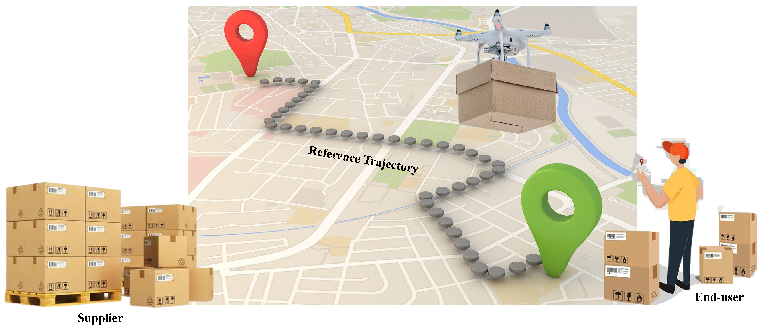
Drones are increasingly being considered as viable alternatives to traditional delivery methods, like trucks and scooters for efficient last-mile delivery to end users. However, implementing drone delivery in supply chains poses various challenges. The final leg of the supply chain, known as the last mile, faces difficulties, such as in traffic congestion, which drones have the potential to overcome. Nevertheless, using drones for this purpose introduces new obstacles related to control and security [1]. The last-mile delivery process is shown in Figure 1.
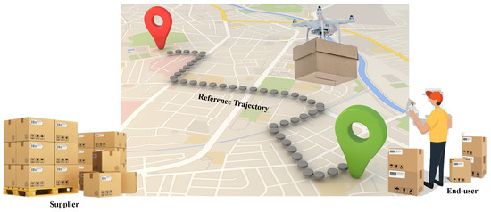
Figure 1.
Last-mile delivery process using drones.
One of the primary challenges in drone delivery is trajectory tracking, as the drone must navigate from the supplier’s location to the end user’s destination accurately. This necessitates the implementation of stable and optimal controllers to ensure smooth and precise flight [2]. Security is also paramount since the drone must avoid collisions with other flying objects, including aircraft and other drones. Additionally, the drone’s operation should adhere to regulations regarding restricted areas and safe landing procedures. To address these security requirements, control laws embedded in the drone platform must reflect considerations, such as obstacle avoidance and maintaining a safe environment [3]. Another crucial aspect is robustness against perturbations and uncertainties encountered during the drone’s journey. These uncertainties can stem from environmental factors, like wind or even cyber attacks that attempt to alter the drone’s trajectory [4]. Ensuring resilience to these perturbations is essential to maintain stability and safety during flight. The successful implementation of drone delivery in logistics and supply chains requires a multidisciplinary approach, encompassing control systems, cybersecurity, and compliance with aviation regulations.
One of the most reliable architectures for ensuring the intended performance is the sliding mode controller. Even though it is based on the law of integer-order law, the sophisticated version, such as the adaptive sliding mode controller, is more robust to parametric uncertainties. In [5], the recent approach of SMC is compared to the last version of the predefined-time terminal sliding mode approach in order to prove its superiority. The last version of the fractional-order predefined-time controller is considered one of the best control techniques for the quadrotor system control due to its offered performances, such as high accuracy and insensitivity to perturbations [5]. The recent approach of SMC is already compared to the last version of the non-integer fractional-order SMC controller and predefined-time terminal sliding mode approach (PTTSMM) in [6]. The results prove the superiority of PTTSMM. The PTTSMM control scheme coped with the disturbances without impacting the tracking control. The section results demonstrated that this controller provides excellent tracking performance compared to the recent SMC approach. The simulation results given in [6] further show that the output has a reasonable steady-error performance.
In recent works, the study of dynamical systems of fractional order has been considered a generalization of integer-order systems. This provides new methodologies for more accurate modeling, robustness, and more flexible control. Distributed-order derivatives can be related to physical properties of dynamical systems that are composed of differential elements with different orders [7]. Sophisticated controllers based on fractional-order computations for quadcopter stabilization have been studied in many works [7].
Several control methods have been developed based on the fractional-order system to improve the tracking performance and robustness of quadrotor systems subjected to disturbances [6]. In order to drive the variables from the arbitrary states to the surface within limited time, a switching control technique based on fractional order is proposed for the control law development in [8]. Compared to other controllers, controller-based fractional-order operators, such as the fixed-time fractional-order sliding mode control [9] and predefined-time terminal sliding mode manifold [6] offer the best tracking performances when the quadrotor system is subject to disturbances.
Despite the recent contributions made in the field of control theory systems, the convergence or stability converging before a predefined time remains a problem under study. The concept of stability in predefined time was presented for a class of dynamic systems in [10]. The variables of the system do not depend on the initial conditions and converge in a fixed predefined time [11]. This predefined convergence time is fixed during the design of the predefined-time controller. The control of fractional-order systems using a fixed time controller was proposed in [12]. Some general classes of fractional-order systems have been proposed in [13,14]. In finite-time convergence or stability, the settling time depends on the initial conditions [15].
Despite the advantages offered by fixed-time controllers [16], it is sometimes difficult to adjust the controller’s gains to obtain the required convergence within a predefined time. The predefined-time controller has been proposed in many works to achieve this objective [17]. To increase the performance of the predefined-time controller, the fractional-order calculus is investigated, such as in [14], in order to enforce the system to converge to the origin within a time that is prescribed as a tunable control parameter, and compensate for the unknown continuous disturbances.
The quadrotor system is considered a complex nonlinear system in terms of parametric uncertainties and disturbances [6]. In this paper, the proposed controller is developed to ensure the high-performance tracking of the variables of the quadrotor under disturbances. The upper bounds of the disturbances must be known to solve the disturbance problems for non-linear systems, such as quadrotor systems. Generally, this limit is rarely known in practice. To solve this problem, the developed controllers are designed, taking this constraint into account. The proposed work uses SMC and fractional computations to inherit the advantages of each one in order to obtain a more robust controller. The new PTFSMC (predefined-time fractional-order sliding mode control) approach is proposed for the control of a quadrotor subjected to external disturbances. The use of a sliding surface based on an integral- and a fractional-order derivative ensures rapid tracking performance and heightened accuracy in attitude and position tracking under disturbances and in the presence of complex trajectories. Furthermore, in order to demonstrate the superiority of the proposed controller, a comparative study with other recent control approaches is analyzed. This comparison shows that the proposed scheme offers better performance in terms of trajectory tracking. As a result, the main contributions of this work are highlighted in the following points: The proposed work uses SMC and fractional calculus to show the advantages of each one. The new predefined-time fractional-order sliding mode control (PTFSMC) approach is proposed for controlling a quadrotor subject to external disturbances. The use of a sliding surface based on the fractional-order integral and derivative allows obtaining an expedited tracking performance and enhanced precision in attitude and position tracking against multiple disturbances and in the presence of complex trajectories. Moreover, in order to demonstrate the superiority of the proposed controller, a comparison study with other recent control approaches is analyzed. From this comparison, it can be seen that the proposed scheme offers better performance in terms of trajectory tracking. Accordingly, the main contributions of this work are highlighted in the following points:
- Predefined-time fractional-order sliding mode manifolds (PTFOSMMs) are investigated for both the attitude and position of the quadrotor.
- A novel control scheme is proposed, which is based on the PTFOSMM manifolds and fractional calculus. According to the Lyapunov theory, global stabilization is ensured, despite the quadrotor being subject to uncertainties and atmospheric disturbances.
- Using the predefined-time fractional-order sliding mode control, many performances are obtained, such as the faster convergence of variables (fractional operators), minimal overshoot, the smallest error, and lower chattering effects, unlike the traditional controller.
- The simulation results demonstrate that the proposed controller allows the quadrotor to complete the desired flight trajectory with high accuracy compared with existing flight controllers, such as the predefined-time terminal sliding mode approach.
2. Preliminary
2.1. Fractional Order Calculus
The fractional order of the derivative and the integrative of fractional calculus can use the Caputo derivative for the function , such as [18].
where and is the derivative order, such that . The Gamma function is defined as follows:
The Caputo operator defined in (3) is the most used for the derivative in fractional-order calculus, where .
But, if , the Caputo derivative can be defined using (4).
Instead of the notation , the Caputo operator is replaced by throughout this paper.
2.2. Predefined-Time Stability
After the development of finite-time stability and fixed-time stability, the predefined time stability is proposed for fast convergence to the origins.
- Finite-time stability [19]: The origin of the steady-state system is finite-time stable if it is asymptotically stable, and any solution of the system reaches the origin at some finite time, this is, , , where is the settling-time function.
- Fixed-time stability [19,20,21,22,23]: The origin of the steady-state system is fixed-time stable if it is finite-time stable and the settling-time function is bounded, i.e., : , .
- Predefined-time stability: The origin of a steady-state system is predefined-time stable if it is fixed-time stable and its variables converge in a predefined time, as demonstrated in Lemma 1.
Lemma 1
([24]). Considering the nonlinear system described, such as , and the positive definite Lyapunov function, , we have the following conditions:
where , , and , with and are positive constants, and is the Gamma function. Then, the considered predefined time is stable and the state variables converge to zero within and .
3. System Modeling
3.1. Dynamics Model of Quadrotor
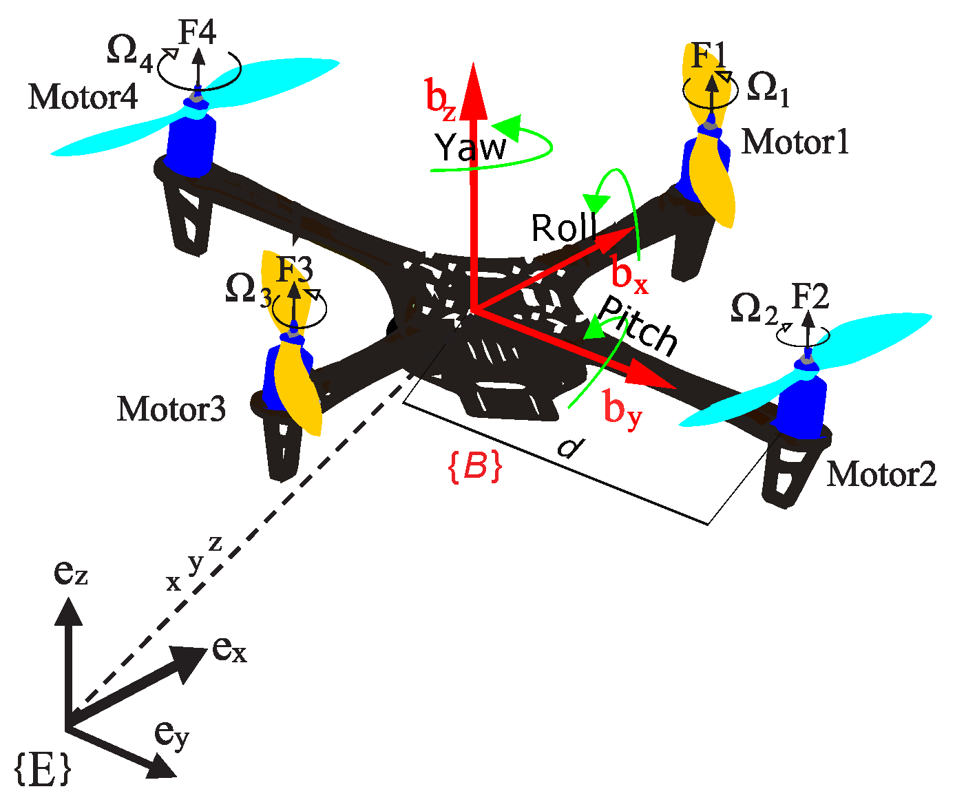
The quadrotor model is given in [6]. The two coordinate frames relative to the quadrotor system are the inertia frame and the body frame , as presented in Figure 2. Using these two coordinate frames, the vectors of quadrotor position and quadrotor attitude can be generated, where , , are, respectively, the roll, pitch, and yaw angles. Using the Newton–Euler formalism, angular velocity , and linear velocity , the dynamic model of the quadrotor under disturbances and parametric uncertainties is developed as follows [6]
where
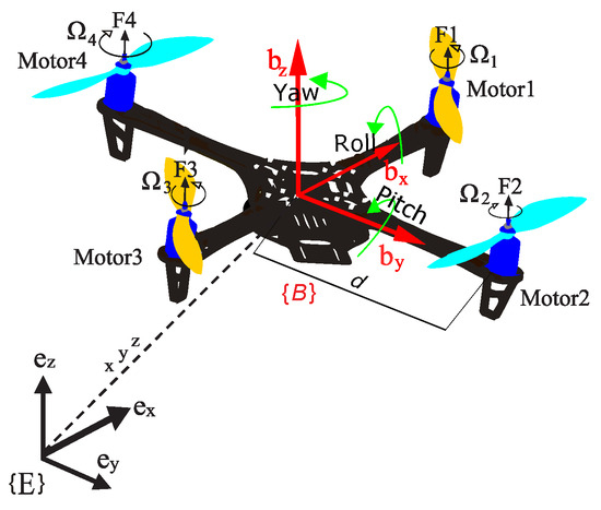
Figure 2.
The four-rotor drone arrangement.
- , with being the total mass and g being the gravity acceleration.
- .
- and are coefficients of the rotational and translational subsystems, respectively.
- is the moment of inertia.
- and are the control input signals.
- are the external disturbances of the position dynamics.
- are the external disturbances of the attitude and position dynamics.
- is the operator of the parameterized uncertainties.
- . l is the distance between the center of mass of the quadrotor of the rotor axis, with c being the drag coefficient.
3.2. Problem Formulation
The model dynamics of a quadrotor under disturbance are developed using the fixed reference frames of the inertial Earth-fixed frame and body-fixed reference frame . The four rotors of the quadrotor can generate the thrust forces versus the angular rotor speed given by: . The parameter depends on the air density and blade geometry. These forces can be investigated to generate control torques given in (8). The total thrust is the sum of the four trust forces ,
where and d are the coefficients of the drag and positive parameter, respectively. The quadrotor dynamic model is developed using some assumptions, given below [25]:
Assumption 1.
The ground effect is ignored. The quadrotor system is stiff, including the blades. The structure of the quadrotor body is symmetrical. Torques and thrust are proportional to the square of the rotor’s rotating speeds.
Remark 1.
To minimize the effect of the load on the drone’s flight, it is important to place the load as symmetrically as possible and place it as close to the center of mass as possible. The proposed controller is robust against uncertain parameters, including the moment of inertia, the mass load, and the drag coefficient. However, the proposed controller is capable of driving the quadrotor and tracking the defined trajectory with the mass load.
The dynamic model of the quadrotor is expressed under disturbances, as follows [6].
Functions and are defined by and , respectively.
with , , , , , , , , , , , , , and .
where for is the state variable of the quadrotor.
The moment of inertia matrix and the drag coefficient are denoted, respectively, by and . The disturbance is considered bounded.
The vehicle control problem is solved by proposing a virtual control input, as given in (10).
According to Equation (10), the total thrust, roll, and pitch angles are given by the following:
Using the virtual control given in (10), the model can be rewritten as
Assumption 2.
The disturbances are considered bounded and meet the inequality , where .
Let us define the tracking errors of the system. For the position loop, the tracking errors are as follows:
For the attitude loop, the tracking errors are as follows:
and the time derivative can be given as follows. For the position loop, the time derivatives of the tracking errors are as follows:
For the attitude loop, the time derivatives of the tracking errors are as follows:
4. Predefined-Time TSM Manifold and the Predefined-Time Stability for the Quadrotor
The quadrotor system is composed of six subsystems, which are like second-order systems. The objective of this section is to design a predefined-time SMC, which converges the quadrotor state variables at a given time. To simplify the controller design, we only present the steps involved in designing the roll controller with its stability, then conclude the other controllers, including the pitch and yaw torques and three virtual position laws, which are for the variables x, y, z, and are denoted by , , and , respectively. Consider the roll subsystem as follows:
with . is the state variable and the torque is the input control. The objective of this paper is to design a new predefined-time controller with fractional dynamics, stabilizing the closed-loop system (17) in the predefined time. To ensure this objective, the FO sliding manifold for (17) is designed as (19),
with and being the constant parameters between 0 and 1, and being the constant parameter.
Consider , the following expression is obtained:
substituting Equation (17) in (20), without perturbation, allows obtaining the equivalent control law:
The reaching controller is designed to make system (17) reach the FO sliding manifolds,
with and being the settling time convergences of the roll system.
Remark 2.
The term in (22) admits a more general design. However, a representative case is illustrated in this paper.
The switching control laws are added in the equivalent control laws to augment the tracking performance and cope with the upper bounds of the disturbances, which are affected in the roll’s subsystem. In addition, the ultimate roll controller is as follows:
Remark 3.
The choice of the Lyapunov function will depend on the specific system being analyzed. However, the general guidelines should be followed in order to ensure that the Lyapunov function is valid.
- The Lyapunov function can be selected to satisfy all the conditions that can be used to prove that the equilibrium point of the system is stable.
- The time derivative of the Lyapunov function should be negative-semidefinite along with the trajectories of the system, meaning that it cannot increase over time.
- The Lyapunov function should also be robust to perturbations in the system, and it should be able to handle multiple equilibrium points and obtain a more flexible control system.
4.1. Predefined-Time Convergence of the -System
For any given time , the proposed predefined-time controller laws aim to drive the system state trajectories to the sliding surface in a predefined time and maintain there for . The reachability in the predefined time is demonstrated in Theorem 1.
Theorem 1.
For a predefined-time constant , the tracking errors with the sliding manifold (19) converge in the predefined time and the settling time, satisfying the following:
Proof.
□
Using the integer-order comparison Lemma, one has , where and
then, using , the following can be obtained:
Therefore, at , the time , which can be computed by integrating (30) from 0 to . Then,
Thus, adopting the change of variable , one has that . Hence,
For and , . Therefore, the variable converges in a predefined time, . where is a predefined time.
4.2. Predefined-Time Stability
The main results of the present paper can be given in Theorem 2.
Theorem 2.
Considering the ϕ-subsystem dynamics controlled by , the adopted surface can be reached in predefined-time . Moreover, the tracking error variables can converge fast to zero in the predefined time.
Proof.
Consider the following Lyapunov function for the -subsystem:
The time-derivative of is expressed as follows:
Substituting the control law V into the -subsystem and differentiating yields the following closed-loop -subsystem.
Then,
Therefore, using Assumption 1, e.g., . Then, (38) is as follows:
with The following assumption can be defined to prove the stability of the system.
Assumption 3.
The disturbance satisfies the following inequality: .
One has the following:
Therefore, using Assumption 1, e.g., . Then, (38) is as follows:
Based on the results of Theorem 1, and (39), the stability of the subsystem is proved with settling time . Finally, from the results of Theorems 1 and 2, the closed-loop subsystem is predefined-time stable, and the settling is . □
In the following part, the ultimate controllers of a quadrotor system are defined.
For pitch motion:
For yaw motion:
For position motion:
For position motion:
For position motion:
5. Simulation Results and Discussion
The performance of the proposed control system is tested in this section using numerical simulation. The simulation results are carried out using MATLAB/Simulink software and the parameters listed in Table 1 and Table 2, in order to show the superiority of the proposed controller in terms of tracking and stability.

Table 1.
Quadrotor parameters.
Table 2.
Control system parameters.
Remark 4.
The fractional-order dynamic approximation used in this article is the CRONE toolbox [26], which was developed in the 1990s by the CRONE team. This method is a MATLAB toolbox developed for fractional operators. Thus, the fractional-order terms in the proposed control approach are approximated using a two-order Oustaloup modified filter with a frequency range from 0.02 to 100 rad/s.
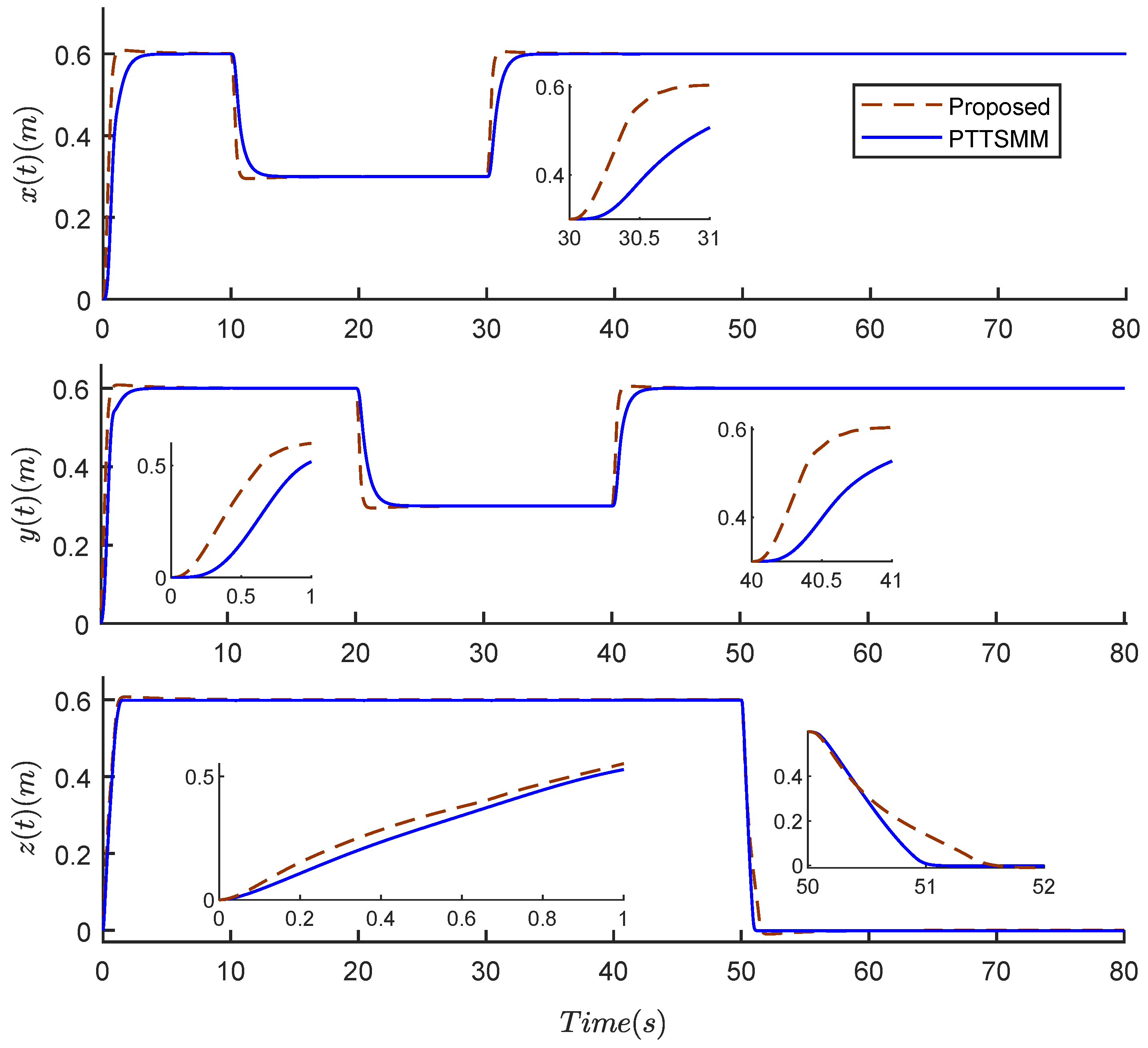
The simulation is achieved using a scenario to track the desired trajectory, as shown in Table 3, using the following starting circumstances: and . The disturbances are chosen for the two scenarios, as shown in (50). Figure 3, the tracking performances of positions x, y, and z of the proposed PTTSMC and PTTSMM under disturbances are presented. The suggested control method, as illustrated in these figures, produces a good tracking trajectory in terms of the fast response and accuracy compared to that of PTTSMM.
Table 3.
The desired reference.
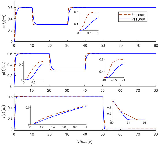
Figure 3.
Positions x, y, z of a quadrotor, using the two compared controllers.
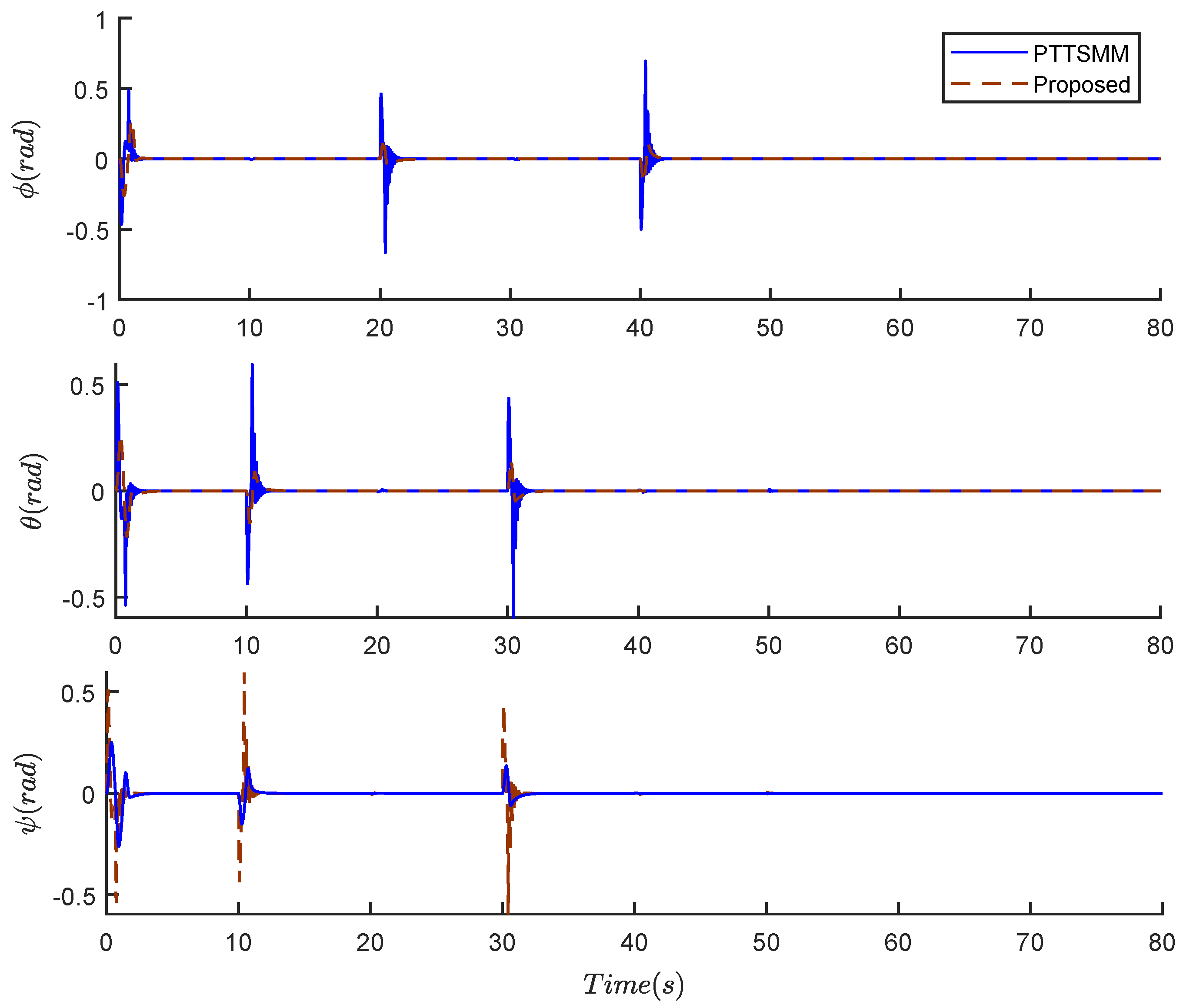
Figure 4 presents the tracking performances of the yaw, pitch, and roll angles using the two compared controllers, which converge to their origin values in finite time.
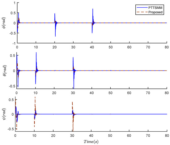
Figure 4.
Roll, pitch, and yaw angles of the quadrotor.
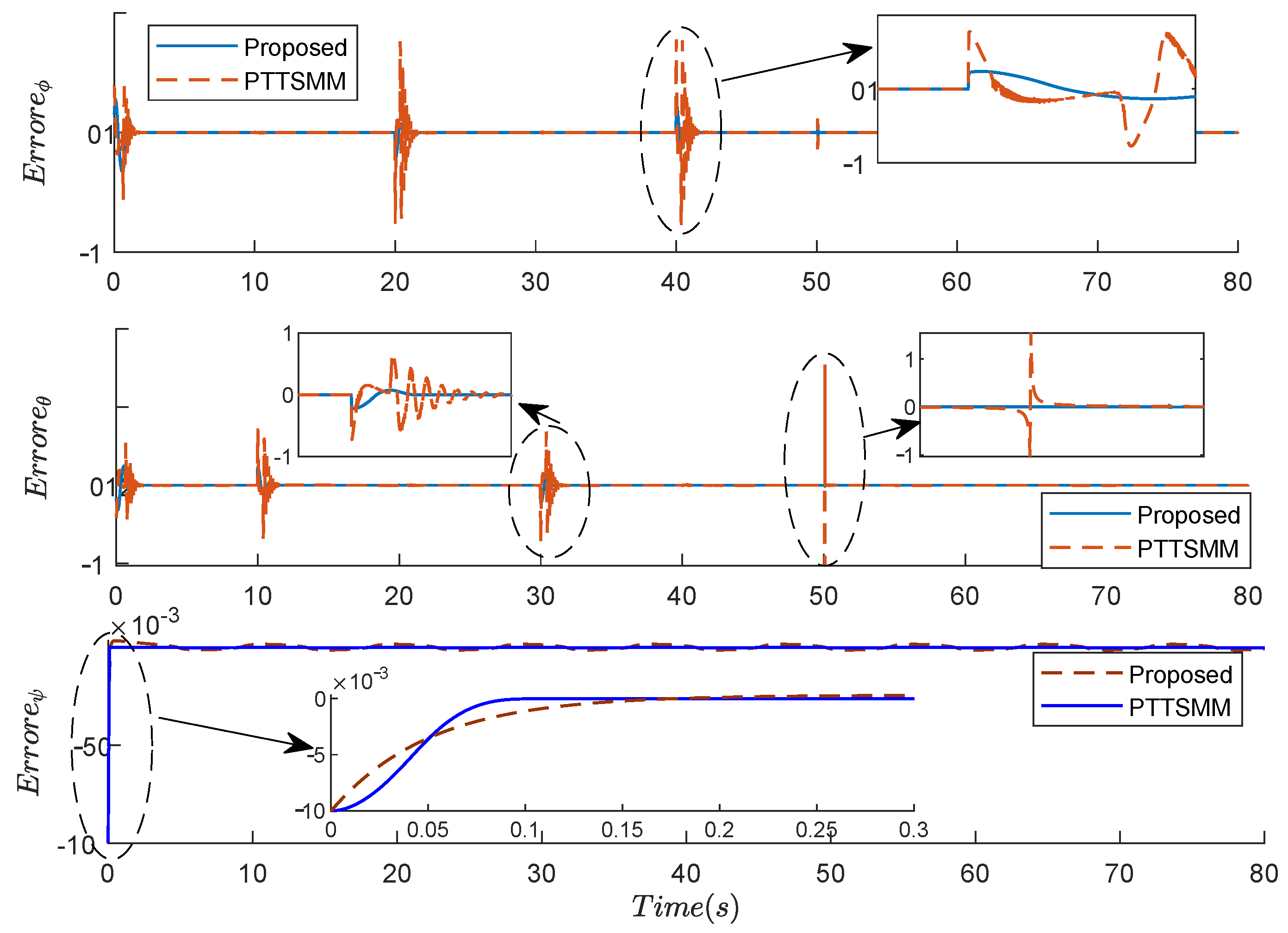
The system’s tracking mistakes are displayed in Figure 5, showing that the tracking errors are nil. From these results, one can see that the pitch angular rapidly returns to zero using the proposed, which demonstrates its superiority compared to the PTTSM M controller.
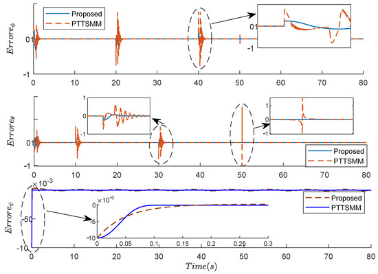
Figure 5.
Results of the angle errors , , and using the two compared controllers.
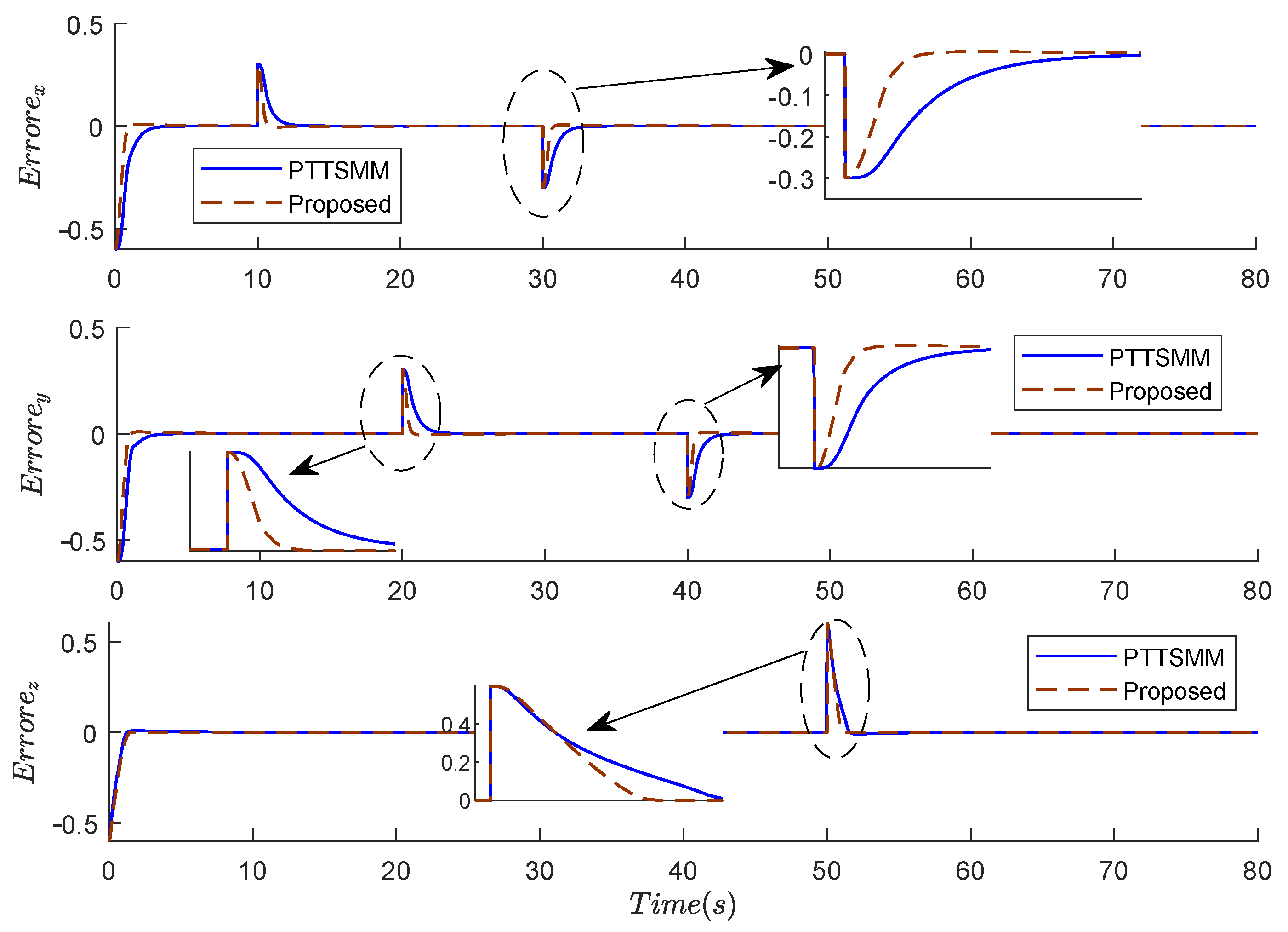
The position errors , , and presented in Figure 6 show that the errors are around zero using the two compared controllers. However, during the step variation of the position, the proposed controller presents the minimum settling time and fast convergence to the desired values.
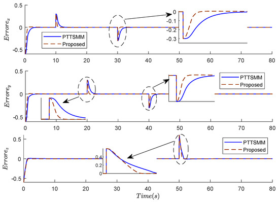
Figure 6.
Results of the errors of positions , , and using the two compared controllers.
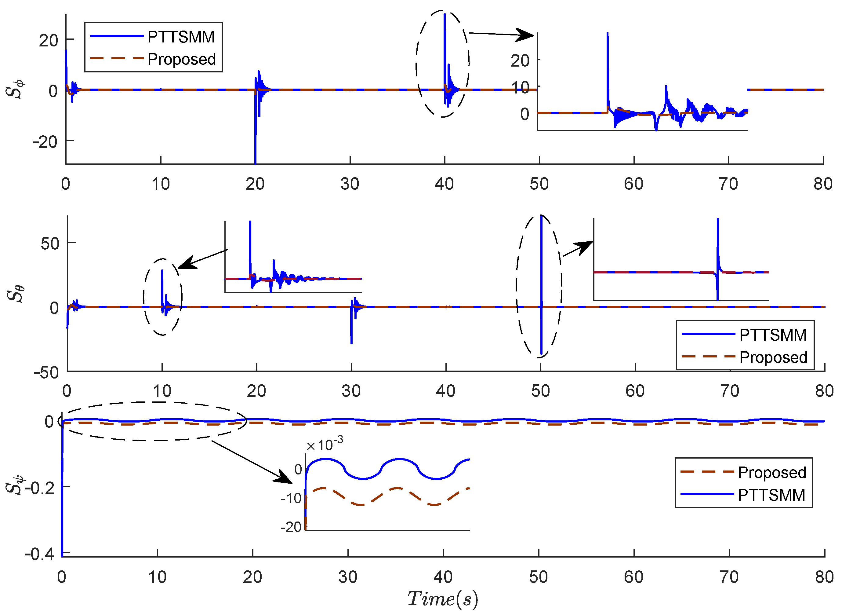
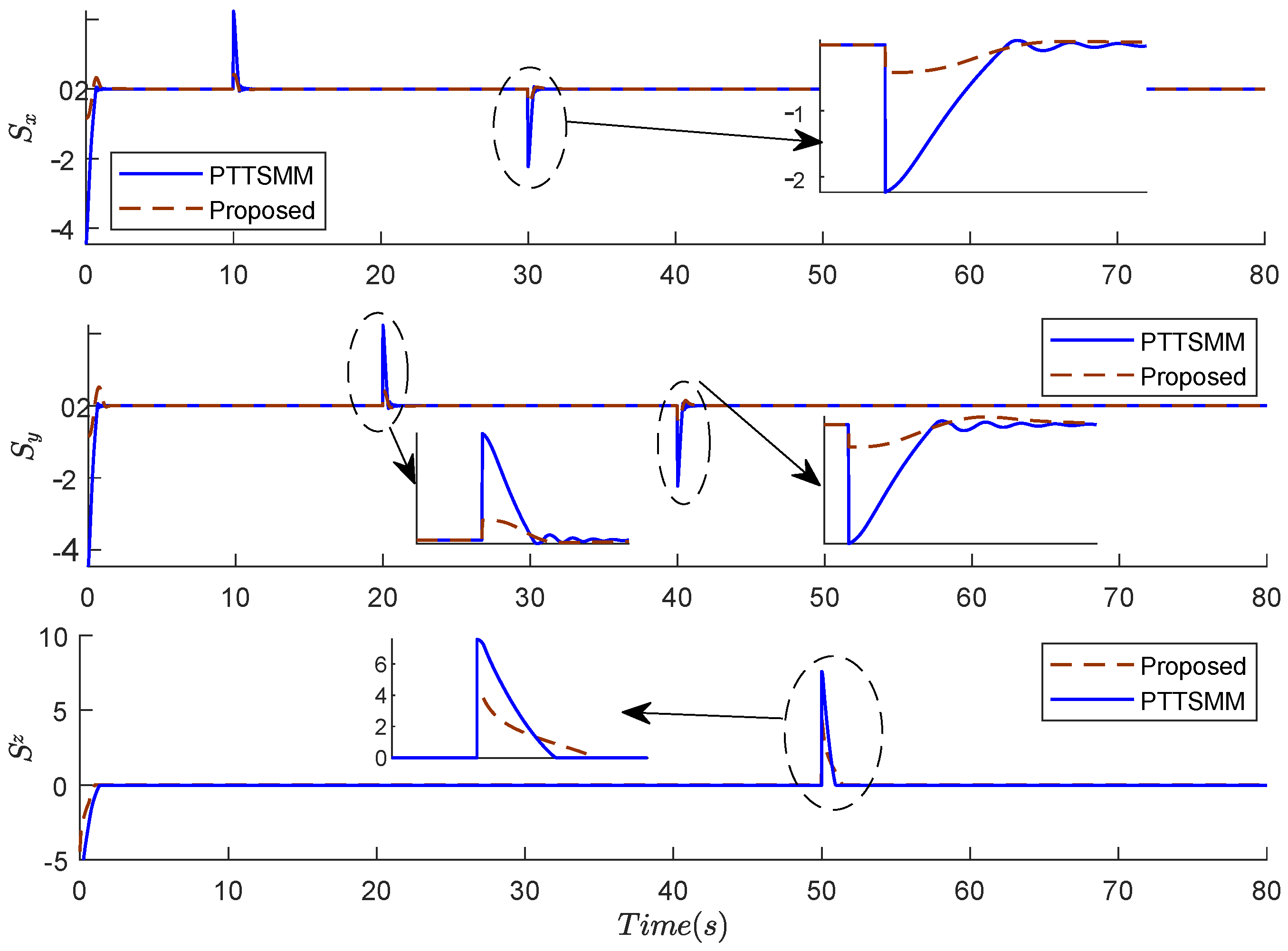
Figure 7 and Figure 8 present the results of the sliding surfaces of angles , , and and positions , , and using the two compared controllers. The proposed controller can generate a sliding surface without ripples and it is rapidly convergent. During the variation steps of the position, the minimal pic and the rapid convergence to zero of the sliding surface are ensured by the proposed controller.
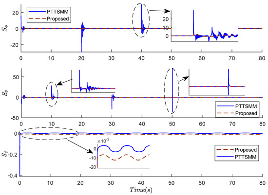
Figure 7.
Results of the sliding surfaces of the angles , , and using the two compared controllers.
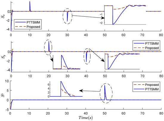
Figure 8.
Results of the sliding surfaces of the positions , , and using the two compared controllers.
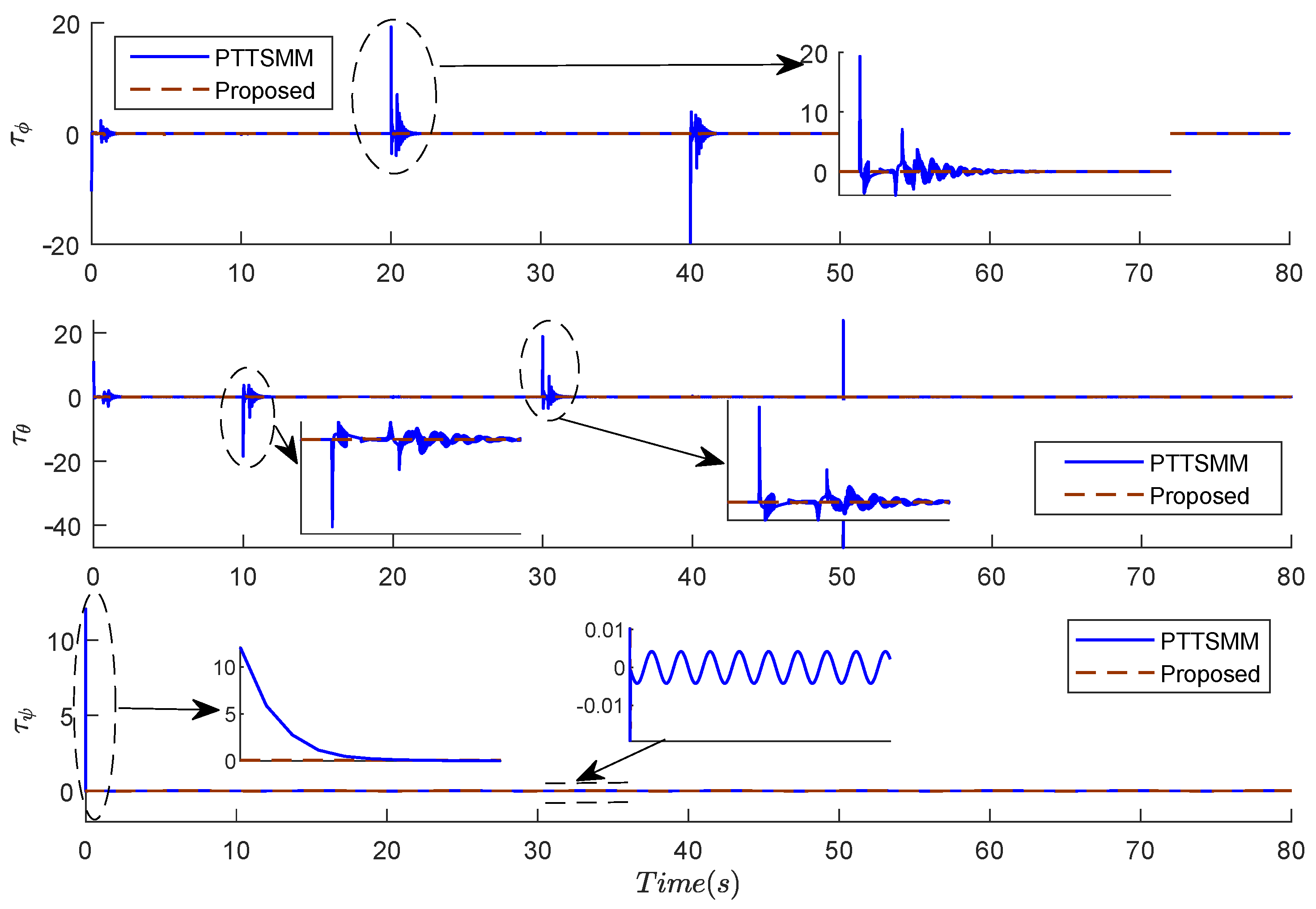
Despite the accuracy and the rapid convergence of errors, the three torques reach steady-state faster without oscillations. The best results of the torques of the roll , pitch , and yaw are obtained using the proposed controller, as shown in Figure 9.

Figure 9.
Results of torques of the roll , pitch , and yaw using the two compared controllers.
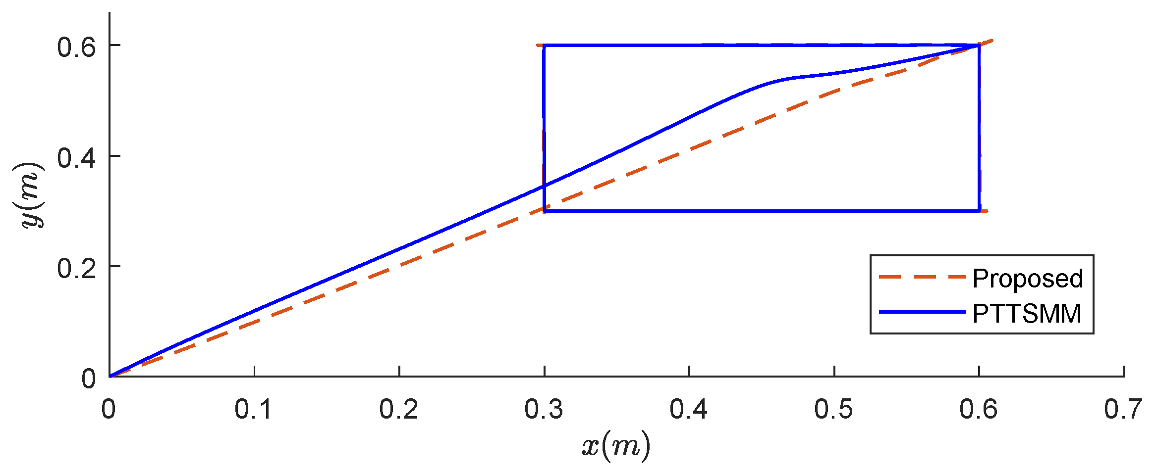
Using the proposed controller, the 2D and 3D trajectories in Figure 10 and Figure 11 exhibit excellent tracking performances compared to that obtained using the PTTSMM controller.
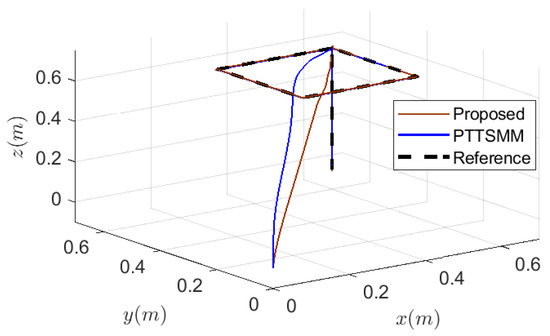
Figure 10.
The 3D trajectories of a quadrotor.
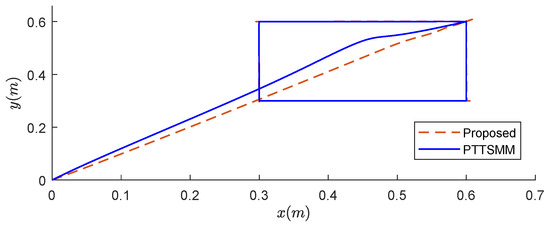
Figure 11.
The 2D trajectories of a quadrotor.
6. Conclusions
This paper presents a novel predefined-time fractional-order sliding mode control for the system of a disturbed quadrotor subjected to perturbation. The tracking errors of positions and attitudes are converged to the newly designed global sliding surface in finite time. The proposed control scheme covered the effects of disturbances without damaging the tracking control. The section results demonstrated that the predefined-time fractional-order sliding mode control offers better tracking performance compared to other control methods. The simulation results further show that the output has a reasonable steady-error performance.
Considering the advantages of the proposed controller, the FTFOSMC holds potential for implementation in other autonomous vehicles, robotics, and electrical systems, promising enhanced performance in the future. Therefore, future work will focus on expanding the control principle to more complicated scenarios, especially those that include multi-model uncertainty and unmatched uncertainty parameters.
Author Contributions
Conceptualization, M.L., K.E., F.S.A. and S.B.; methodology, K.E. and M.L.; software, M.L.; validation, K.E., M.L., S.B., F.S.A. and S.K.; formal analysis, M.L.; investigation, M.L.; resources, M.L.; data curation, M.L. and K.E.; writing—original draft preparation, M.L., S.B. and S.K.; writing—review and editing, M.L., S.B. and S.K.; visualization, M.L., S.B. and S.K.; supervision, M.L., S.B., F.S.A. and S.K.; project administration, S.B. and S.K.; funding acquisition, M.L., S.B. and S.K. All authors have read and agreed to the published version of the manuscript.
Funding
Deputyship for Research & Innovation, Ministry of Education in Saudi Arabia—project number MoE-IF-UJ-22-04220772-3.
Data Availability Statement
Data from this paper are presented in Section 5.
Acknowledgments
The authors extend their appreciation to the Deputyship for Research & Innovation, Ministry of Education in Saudi Arabia for funding this research work through the project number MoE-IF-UJ-22-04220772-3.
Conflicts of Interest
The authors declare no conflict of interest.
References
- Verling, S.; Glavin, M.; Jones, E. A survey of drone delivery systems. Int. J. Eng. Technol. (IJET) 2017, 9, 200–208. [Google Scholar]
- Pournader, M.; Gopalakrishnan, G.; How, J.P. Robust trajectory tracking for the quadrotors: A fast model predictive control approach. IEEE Robot. Autom. Lett. 2018, 3, 3388–3395. [Google Scholar]
- Xu, Y.; Wu, J.; Li, X.; Wang, M. A survey on collision avoidance for drones. IET Cyber-Phys. Syst. Theory Appl. 2019, 4, 217–228. [Google Scholar]
- Mendes, T.S.; Maza, I.; Cabreira, M.C. Robust trajectory tracking of autonomous UAVs using sliding mode control. IFAC-PapersOnLine 2018, 51, 222–227. [Google Scholar]
- Labbadi, M.; Cherkaoui, M. Adaptive Fractional-Order Nonsingular Fast Terminal Sliding Mode Based Robust Tracking Control of Quadrotor UAV With Gaussian Random Disturbances and Uncertainties. IEEE Trans. Aerosp. Electron. Syst. 2021, 57, 2265–2277. [Google Scholar] [CrossRef]
- Labbadi, M.; Elyaalaoui, K.; Dabachi, M.A.; Lakrit, S.; Djemai, M.; Cherkaoui, M. Robust flight control for a quadrotor under external disturbances based on predefined-time terminal sliding mode manifold. J. Vib. Control 2022, 29, 2064–2076. [Google Scholar] [CrossRef]
- Lavın-Delgado, J.E.; Beltran, Z.Z.; Gomez-Aguilar, J.F. Eduardo Perez-Careta, Controlling a quadrotor UAV by means of a fractional nested saturation control. Adv. Space Res. 2022, 71, 3822–3836. [Google Scholar] [CrossRef]
- Shi, X.; Cheng, Y.; Yin, C.; Zhong, S.; Huang, X.; Chen, K.; Qiu, G. Adaptive Fractional-Order SMC Controller Design for Unmanned Quadrotor Helicopter Under Actuator Fault and Disturbances. IEEE Access 2020, 8, 103792–103802. [Google Scholar] [CrossRef]
- Huang, S.; Wang, J.; Huang, C.; Zhou, L.; Xiong, L.; Liu, J.; Li, P. A fixed-time fractional-order sliding mode control strategy for power quality enhancement of PMSG wind turbine. Int. J. Electr. Power Energy Syst. 2022, 134, 107354. [Google Scholar] [CrossRef]
- Jiménez-Rodríguez, E.; Muñoz-Vázquez, A.J.; Sánchez-Torres, J.D.; Defoort, M.; Loukianov, A.G. A Lyapunov-Like Characterization of Predefined-Time Stability. IEEE Trans. Autom. Control 2020, 65, 4922–4927. [Google Scholar] [CrossRef]
- Polyakov, A.; Fridman, L. Stability notions and Lyapunov functions for sliding mode control systems. J. Frankl. Inst. 2014, 351, 1831–1865. [Google Scholar] [CrossRef]
- Shirkavand, M.; Pourgholi, M. Robust fixed-time synchronization of fractional order chaotic using free chattering nonsingular adaptive fractional sliding mode controller design. Chaos Solitons Fractals 2018, 113, 135–147. [Google Scholar] [CrossRef]
- Muñoz-Vázquez, A.J.; Sánchez-Torres, J.D.; Defoort, M.; Boulaaras, S. Predefined-time convergence in fractional-order systems. Chaos Solitons Fractals 2021, 143, 110571. [Google Scholar] [CrossRef]
- Muñoz-Vázquez, A.J.; Sánchez-Torres, J.D.; Defoort, M. Second-order predefined-time sliding-mode control of fractional-order systems. Asian J. Control 2020, 24, 74–82. [Google Scholar] [CrossRef]
- Ge, M.F.; Liu, Z.W.; Wen, G.; Yu, X.; Huang, T. Hierarchical controller-estimator for coordination of networked Euler–Lagrange systems. IEEE Trans. Cybern. 2019, 50, 2450–2461. [Google Scholar] [CrossRef] [PubMed]
- Polyakov, A. Nonlinear feedback design for fixed-time stabilization of linear control systems. IEEE Trans. Autom. Control 2011, 57, 2106–2110. [Google Scholar] [CrossRef]
- Sánchez-Torres, J.D.; Gómez-Gutiérrez, D.; López, E.; Loukianov, A.G. A class of predefined-time stable dynamical systems. IMA J. Math. Control Inf. 2018, 35, i1–i29. [Google Scholar] [CrossRef]
- Das, S. Functional Fractional Calculus for System Identification and Controls; Springer: Heidelberg, Germany, 2008. [Google Scholar]
- Zhou, B. Finite-time stabilization of linear systems by bounded linear time-varying feedback. Automatica 2020, 113, 108760. [Google Scholar] [CrossRef]
- Zhou, B.; Michiels, W.; Chen, J. Fixed-time stabilization of linear delay systems by smooth periodic delayed feedback. IEEE Trans. Autom. Control 2021, 67, 557–573. [Google Scholar] [CrossRef]
- Yu, S.; Yu, X.; Stonier, R. Continuous finite-time control for robotic manipulators with terminal sliding modes. In Proceedings of the 6th International Conference on Information Fusion, Cairns, Australia, 8–11 July 2003; Volume 2, pp. 1433–1440. [Google Scholar] [CrossRef]
- Zuo, Z. Nonsingular fixed-time consensus tracking for second-order multi-agent networks. Automatica 2015, 54, 305–309. [Google Scholar] [CrossRef]
- Zuo, Z. Non-singular fixed-time terminal sliding mode control of non-linear systems. IET Control Theory Appl. 2015, 9, 545–552. [Google Scholar] [CrossRef]
- Hong, Y.; Huang, J.; Xu, Y. On an output feedback finite-time stabilization problem. IEEE Trans. Autom. Control 2001, 46, 305–309. [Google Scholar] [CrossRef]
- Labbadi, M.; Cherkaoui, M. Robust adaptive nonsingular fast terminal sliding-mode tracking control for an uncertain quadrotor UAV subjected to disturbances. In ISA Transactions; Elsevier: Amsterdam, The Netherlands, 2020; Volume 99, pp. 290–304. [Google Scholar] [CrossRef]
- Oustaloup, A.; Melchior, P.; Lanusse, P.; Cois, O.; Dancla, F. The CRONE toolbox for matlab, CACS D. In Proceedings of the IEEE International Symposium on Computer-Aided Control System Design (Cat. No.00TH8537), Anchorage, AK, USA, 25–27 September 2000; pp. 190–195. [Google Scholar] [CrossRef]

Disclaimer/Publisher’s Note: The statements, opinions and data contained in all publications are solely those of the individual author(s) and contributor(s) and not of MDPI and/or the editor(s). MDPI and/or the editor(s) disclaim responsibility for any injury to people or property resulting from any ideas, methods, instructions or products referred to in the content. |
© 2023 by the authors. Licensee MDPI, Basel, Switzerland. This article is an open access article distributed under the terms and conditions of the Creative Commons Attribution (CC BY) license (https://creativecommons.org/licenses/by/4.0/).