
A Location-Based Crowdsensing Incentive Mechanism Based on Ensemble Learning and Prospect Theory


Abstract
:1. Introduction
2. Related Work
2.1. Current Study of Incentive Mechanisms for Crowdsensing
2.2. Current Study of Ensemble Learning
2.3. Current Study of Prospect Theory
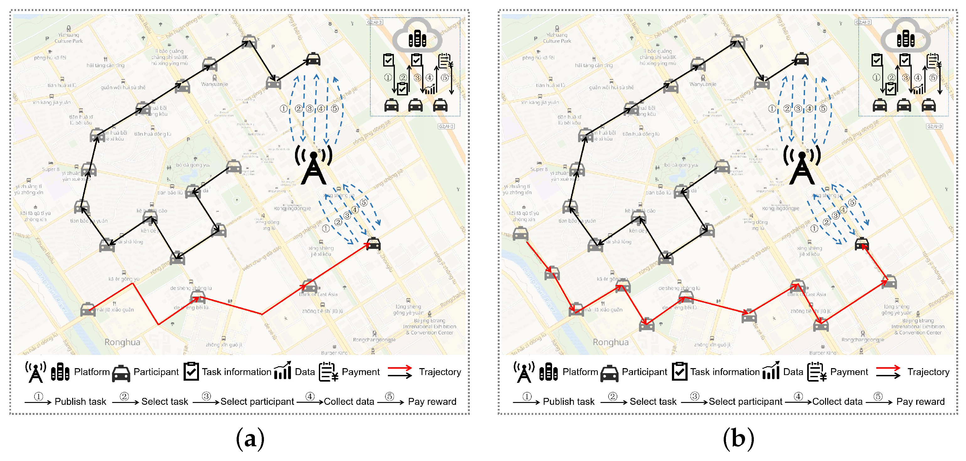
3. System Model
- The platform publishes tasks. The platform will publish the task information to the participants, including the quality of data to be collected, the reward the platform can provide, etc. The platform will first use the DSGD to predict whether the participant is a long-term or short-term participant and then provide the relevant information to the participant using different mechanisms respectively;
- Participants select the task. Participants decide whether to accept a task based on their consideration of reward and cost. Different types of participants are motivated by different mechanisms, where short-term participants are motivated by the SPIMPT, and long-term participants are motivated by the LPIM;
- Platform selects participants. After the platform receives the participant’s decision, it will select the appropriate participants from the participants who are willing to participate in the task;
- The participants complete the tasks. The participants collect data and send the collected data to the platform;
- The platform pays rewards. The platform pays short-term participants according to the SPIMPT and long-term participants according to the LPIM.
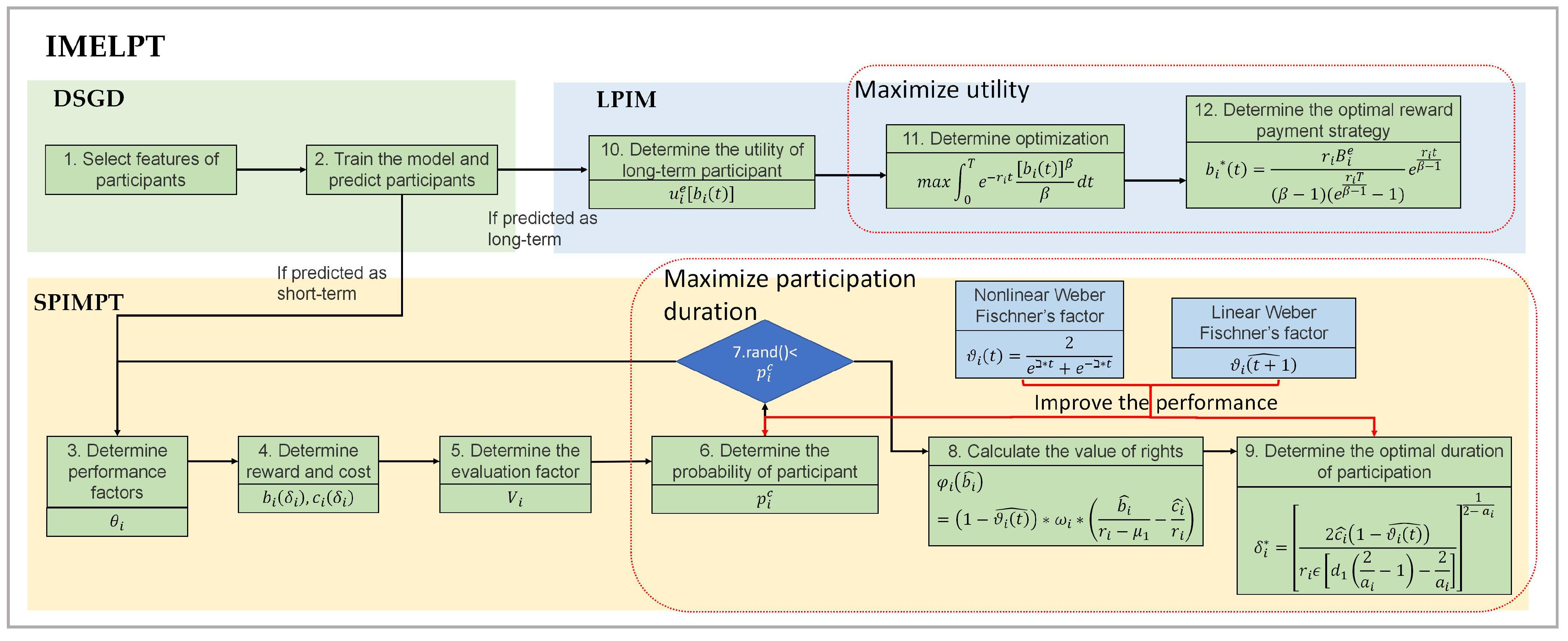
Logical Model
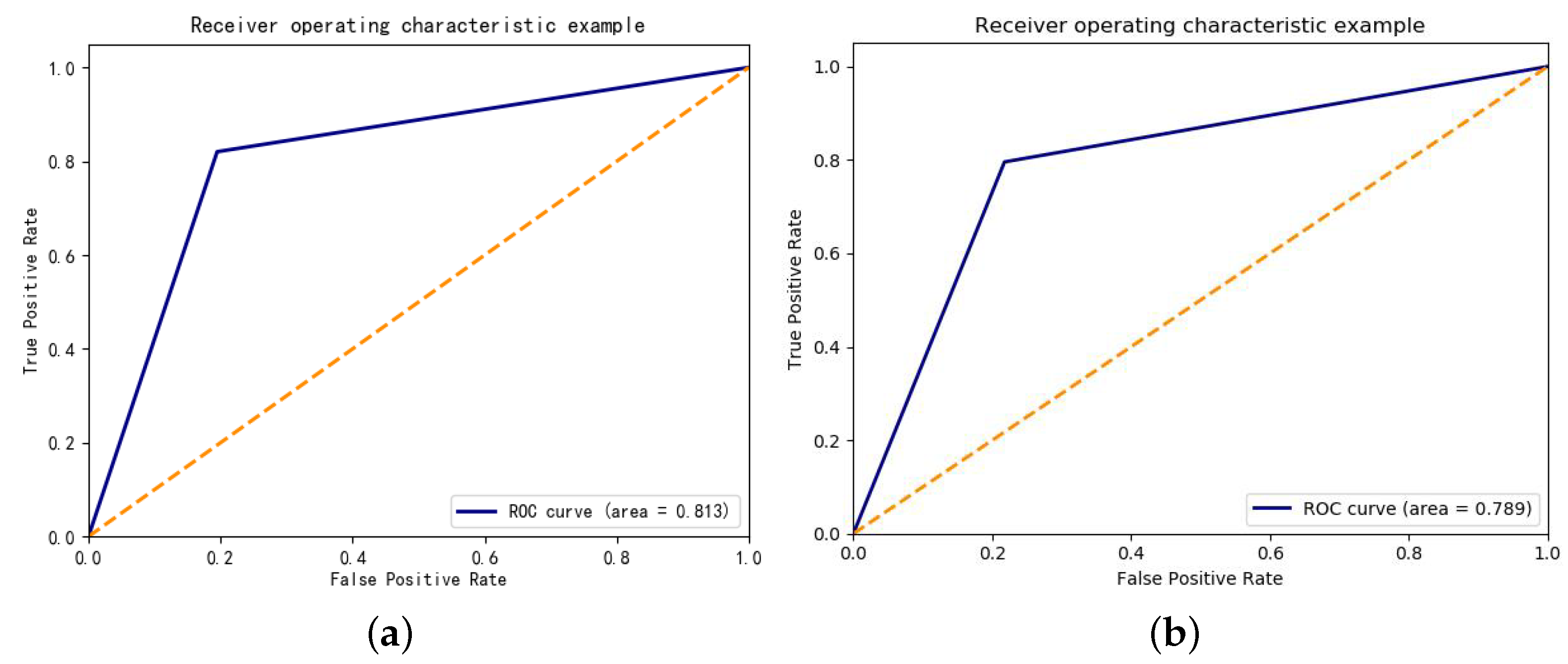
4. Detail of the DSGD
5. Discussion of the Participant Incentive Mechanism
5.1. Cultivation Mechanism for Short-Term Participants
5.1.1. Design of Cultivation Mechanism Based on Prospect Theory
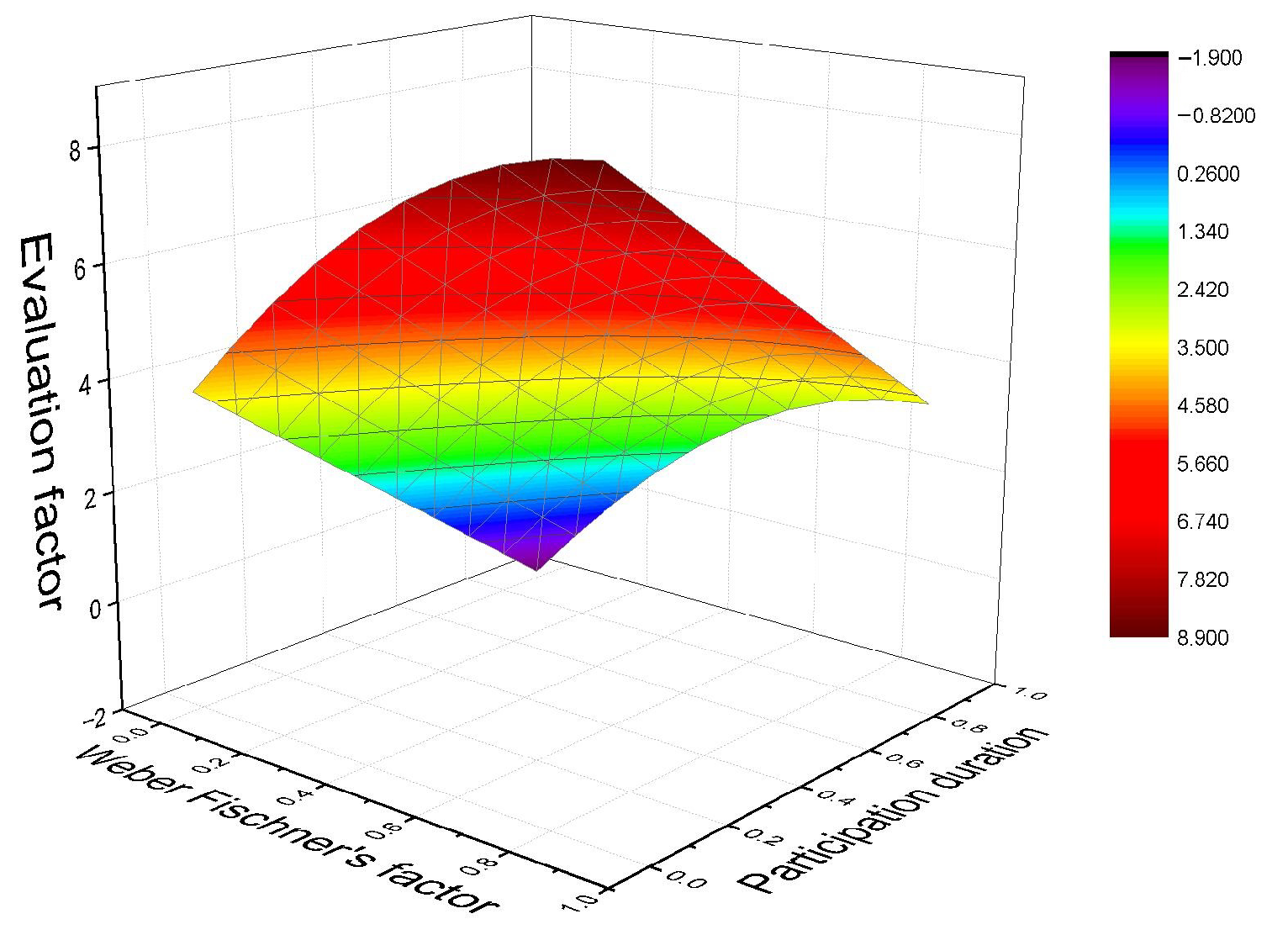
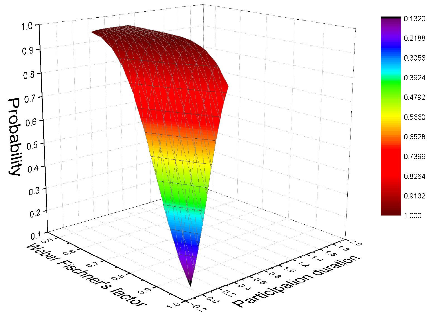
5.1.2. Impact of Prospect Factor on Participants’ Decisions
5.2. Maintenance Mechanism for Short-Term Participants
5.2.1. Design of Maintenance Mechanism Based on Prospect Theory
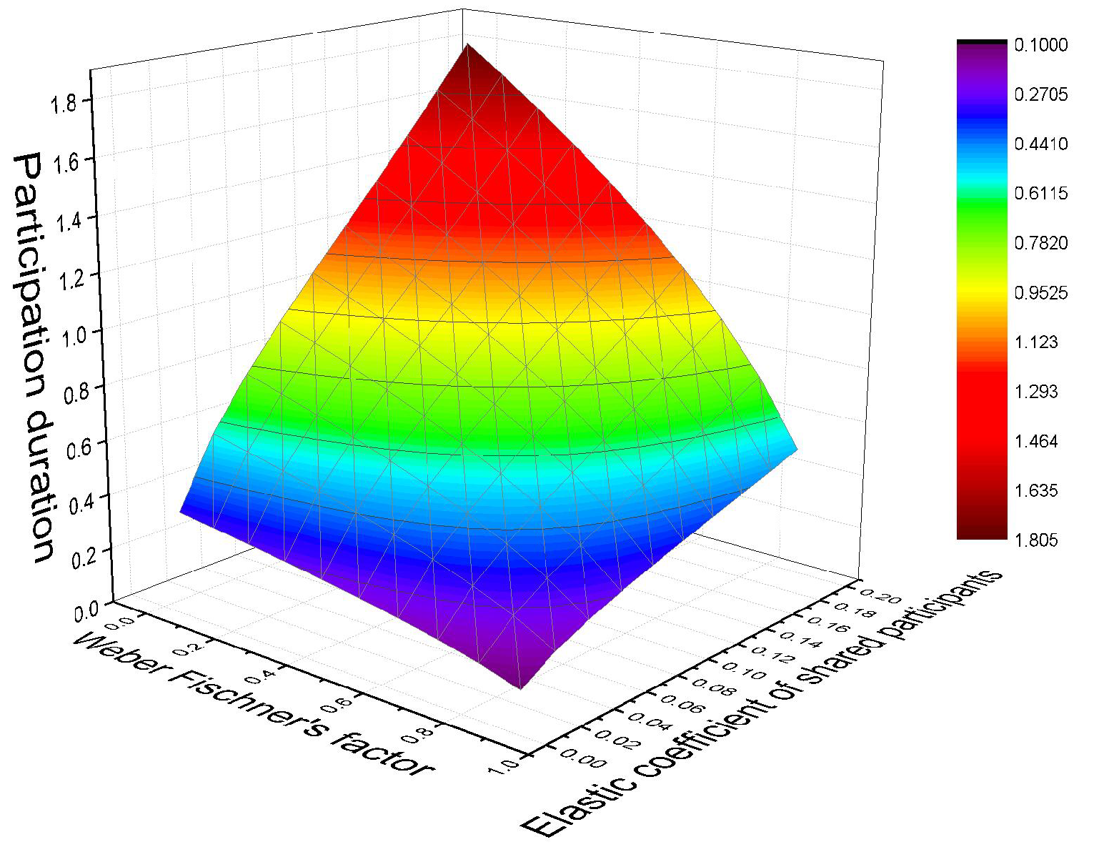
5.2.2. Optimal Decision-Making of Participants in the Maintenance Mechanism
5.3. Incentive Mechanism for Long-Term Participant
6. Experiment and Analysis
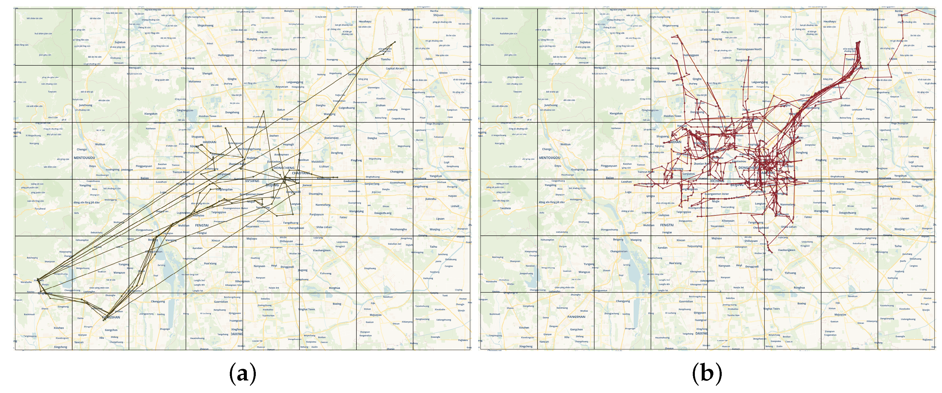
6.1. Setup of the Experiment
6.2. Evaluation of the IMELPT
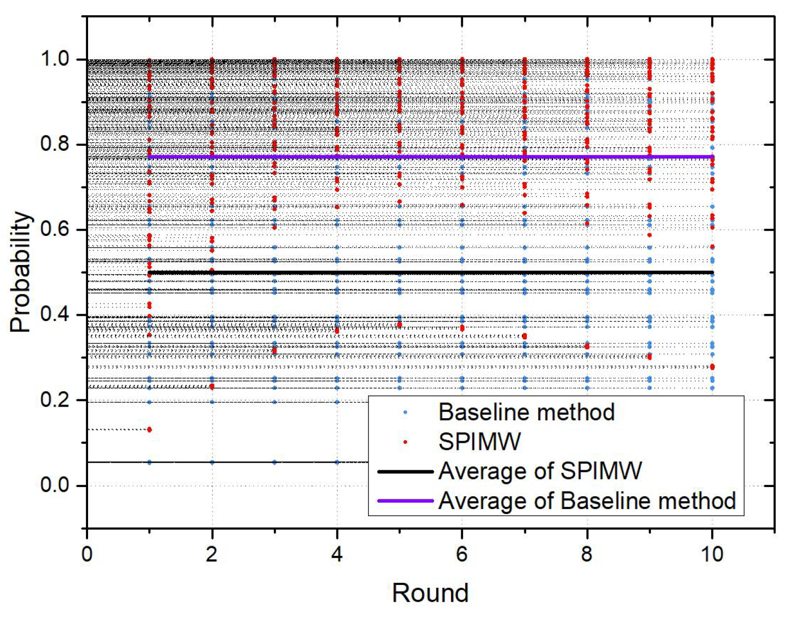
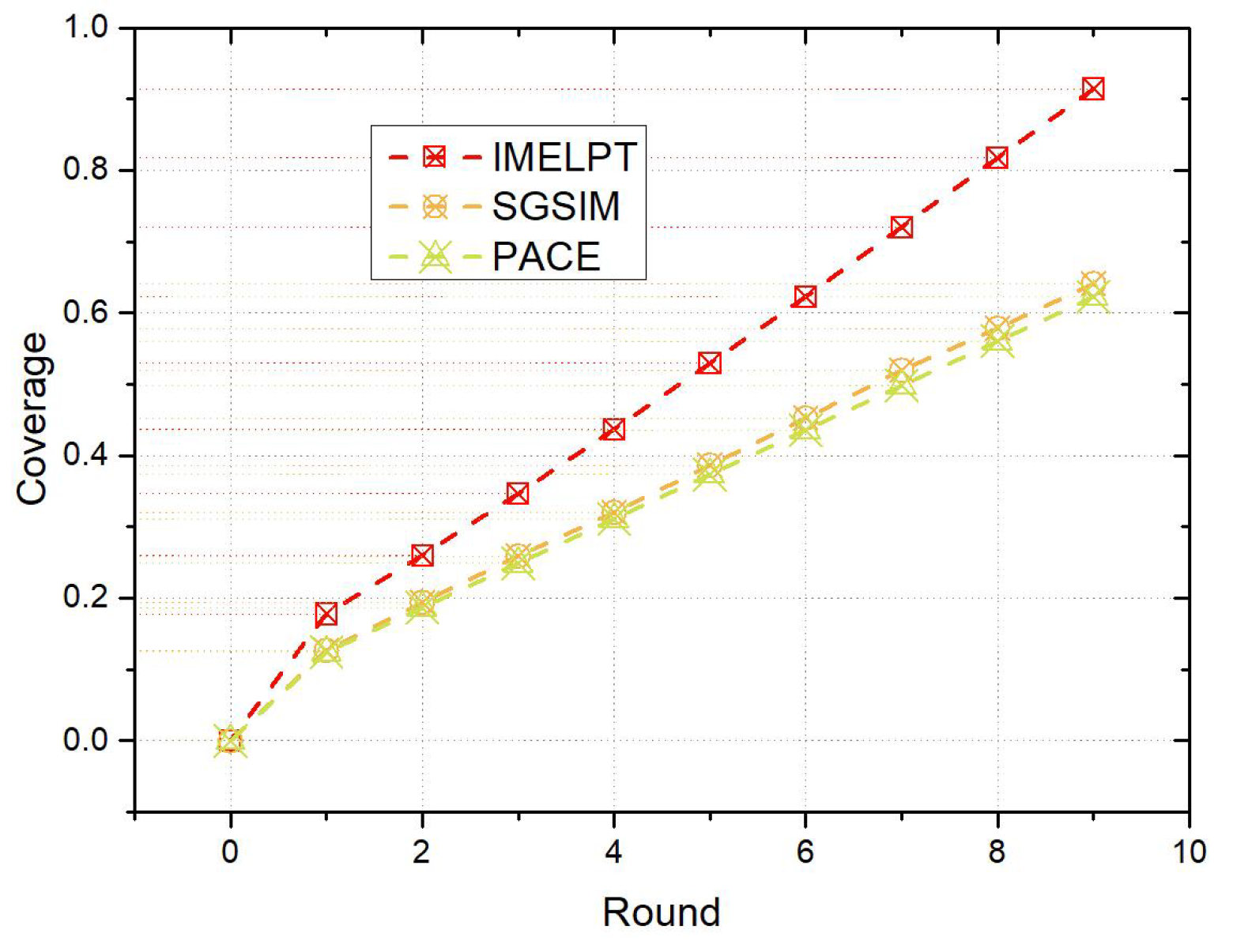
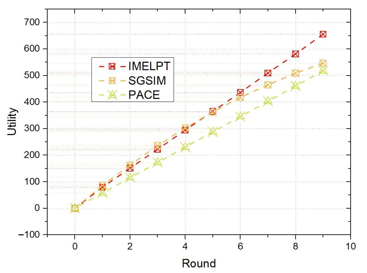
6.3. Comparison of the IMELPT
7. Conclusions
Author Contributions
Funding
Institutional Review Board Statement
Informed Consent Statement
Data Availability Statement
Conflicts of Interest
Abbreviations
| IMELPT | Incentive Mechanism based on Ensemble Learning and Prospect Theory |
| DSGD | Deep-Stacking-Generation algorithm based on Dropout |
| SPIMPT | Short-term Participant Incentive Mechanism based on Prospect Theory |
| LPIM | Long-term Participant Incentive Mechanism |
References
- Tan, W.; Zhao, L.; Li, B.; Xu, L.; Yang, Y. Multiple Cooperative Task Allocation in Group-Oriented Social Mobile Crowdsensing. IEEE Trans. Serv. Comput. 2022, 15, 3387–3401. [Google Scholar] [CrossRef]
- Li, L.; Shi, D.; Zhang, X.; Hou, R.; Yue, H.; Li, H.; Pan, M. Privacy Preserving Participant Recruitment for Coverage Maximization in Location Aware Mobile Crowdsensing. IEEE Trans. Mob. Comput. 2022, 21, 3250–3262. [Google Scholar] [CrossRef]
- Chen, F.; Huang, L.; Gao, Z.; Liwang, M. Latency-Sensitive Task Allocation for Fog-Based Vehicular Crowdsensing. IEEE Syst. J. 2022, 17, 1909–1917. [Google Scholar] [CrossRef]
- Ramazani, A.; Vahdat-Nejad, H. CANS: Context-aware traffic estimation and navigation system. IET Intell. Transp. Syst. 2017, 11, 326–333. [Google Scholar] [CrossRef]
- Xu, J.; Yang, S.; Lu, W.; Xu, L.; Yang, D. Incentivizing for Truth Discovery in Edge-assisted Large-scale Mobile Crowdsensing. Sensors 2020, 20, 805. [Google Scholar] [CrossRef]
- Liu, W.; Yang, Y.; Wang, E.; Wang, H.; Wang, Z.; Wu, J. Dynamic online user recruitment with (non-) submodular utility in mobile crowdsensing. IEEE-ACM Trans. Netw. 2021, 29, 2156–2169. [Google Scholar] [CrossRef]
- Restuccia, F.; Ferraro, P.; Silvestri, S.; Das, S.K.; Lo Re, G. IncentMe: Effective Mechanism Design o Stimulate Crowdsensing Participants with Uncertain Mobility. IEEE Trans. Mob. Comput. 2019, 18, 1571–1584. [Google Scholar] [CrossRef]
- Zhao, B.; Tang, S.; Liu, X.; Zhang, X. PACE: Privacy-Preserving and Quality-Aware Incentive Mechanism for Mobile Crowdsensing. IEEE Trans. Mob. Comput. 2021, 20, 1924–1939. [Google Scholar] [CrossRef]
- Xu, J.; Zhou, Y.; Ding, Y.; Yang, D.; Xu, L. Biobjective Robust Incentive Mechanism Design for Mobile Crowdsensing. IEEE Internet Things J. 2021, 8, 14971–14984. [Google Scholar] [CrossRef]
- Xu, C.; Si, Y.; Zhu, L.; Zhang, C.; Sharif, K.; Zhang, C. Pay as How You Behave: A Truthful Incentive Mechanism for Mobile Crowdsensing. IEEE Internet Things J. 2019, 6, 10053–10063. [Google Scholar] [CrossRef]
- Xu, X.; Yang, Z.; Xian, Y. ATM: Attribute-Based Privacy-Preserving Task Assignment and Incentive Mechanism for Crowdsensing. IEEE Access 2021, 9, 60923–60933. [Google Scholar] [CrossRef]
- Zhan, Y.; Xia, Y.; Liu, Y.; Li, F.; Wang, Y. Incentive-Aware Time-Sensitive Data Collection in Mobile Opportunistic Crowdsensing. IEEE Trans. Veh. Technol. 2017, 66, 7849–7861. [Google Scholar] [CrossRef]
- Lu, J.; Zhang, Z.; Wang, J.; Li, R.; Wan, S. A Green Stackelberg-game Incentive Mechanism for Multi-service Exchange in Mobile Crowdsensing. ACM Trans. Internet Technol. 2022, 22, 31. [Google Scholar] [CrossRef]
- Ren, Y.; Li, X.; Miao, Y.; Luo, B.; Weng, J.; Choo, K.K.R.; Deng, R.H. Towards Privacy-Preserving Spatial Distribution Crowdsensing: A Game Theoretic Approach. IEEE Trans. Inf. Forensics Secur. 2022, 17, 804–818. [Google Scholar] [CrossRef]
- Wang, W.; Zhan, J.; Herrera-Viedma, E. A three-way decision approach with a probability dominance relation based on prospect theory for incomplete information systems. Inf. Sci. 2022, 611, 199–224. [Google Scholar] [CrossRef]
- Liu, C.; Du, R.; Wang, S.; Bie, R. Cooperative Stackelberg game based optimal allocation and pricing mechanism in crowdsensing. Int. J. Sens. Netw. 2018, 28, 57–68. [Google Scholar] [CrossRef]
- Han, M.; Li, X.; Wang, L.; Zhang, N.; Cheng, H. Review of ensemble classification over data streams based on supervised and semi-supervised. J. Intell. Fuzzy Syst. 2022, 43, 3859–3878. [Google Scholar] [CrossRef]
- Gan, L.; Hu, Y.; Chen, X.; Li, G.; Yu, K. Application and Outlook of Prospect Theory Applied to Bounded Rational Power System Economic Decisions. IEEE Trans. Ind. Appl. 2022, 58, 3227–3237. [Google Scholar] [CrossRef]
- Yang, J.; Fu, L.; Yang, B.; Xu, J. Participant Service Quality Aware Data Collecting Mechanism With High Coverage for Mobile Crowdsensing. IEEE Access 2020, 8, 10628–10639. [Google Scholar] [CrossRef]
- Liu, Y.; Li, Y.; Cheng, W.; Wang, W.; Yang, J. A willingness-aware user recruitment strategy based on the task attributes in mobile crowdsensing. Int. J. Distrib. Sens. Netw. 2022, 18, 15501329221123531. [Google Scholar] [CrossRef]
- Zhang, J.; Yang, X.; Feng, X.; Yang, H.; Ren, A. A Joint Constraint Incentive Mechanism Algorithm Utilizing Coverage and Reputation for Mobile Crowdsensing. Sensors 2020, 20, 4478. [Google Scholar] [CrossRef] [PubMed]
- Gu, Y.; Shen, H.; Bai, G.; Wang, T.; Liu, X. QoI-aware incentive for multimedia crowdsensing enabled learning system. Multimed. Syst. 2020, 26, 3–16. [Google Scholar] [CrossRef]
- Chen, X.; Xu, S.; Han, J.; Fu, H.; Pi, X.; Joe-Wong, C.; Li, Y.; Zhang, L.; Noh, H.Y.; Zhang, P. PAS: Prediction-Based Actuation System for City-Scale Ridesharing Vehicular Mobile Crowdsensing. IEEE Internet Things J. 2020, 7, 3719–3734. [Google Scholar] [CrossRef]
- Song, S.; Liu, Z.; Li, Z.; Xing, T.; Fang, D. Coverage-Oriented Task Assignment for Mobile Crowdsensing. IEEE Internet Things J. 2020, 7, 7407–7418. [Google Scholar] [CrossRef]
- Mohammadi, S.; Narimani, Z.; Ashouri, M.; Firouzi, R.; Karimi-Jafari, M.H. Ensemble learning from ensemble docking: Revisiting the optimum ensemble size problem. Sci. Rep. 2022, 12, 410. [Google Scholar] [CrossRef]
- Wang, P.; Chen, Z.; Deng, X.; Wang, J.; Tang, R.; Li, H.; Hong, S.; Wu, Z. The Prediction of Storm-Time Thermospheric Mass Density by LSTM-Based Ensemble Learning. Space-Weather.-Int. J. Res. Appl. 2022, 20, e2021SW002950. [Google Scholar] [CrossRef]
- Wang, X.; Han, T. Transformer Fault Diagnosis Based on Stacking Ensemble Learning. IEEJ Trans. Electr. Electron. Eng. 2020, 15, 1734–1739. [Google Scholar] [CrossRef]
- Wang, H.; Zhao, Y. ML2E: Meta-Learning Embedding Ensemble for Cold-Start Recommendation. IEEE Access 2020, 8, 165757–165768. [Google Scholar] [CrossRef]
- Gelbrich, K.; Roschk, H. Do complainants appreciate overcompensation? A meta-analysis on the effect of simple compensation vs. overcompensation on post-complaint satisfaction. Mark. Lett. 2011, 22, 31–47. [Google Scholar] [CrossRef]
- Wang, Y.; Fan, R.; Du, K.; Lin, J.; Wang, D.; Wang, Y. Private charger installation game and its incentive mechanism considering prospect theory. Transp. Res. Part-Transp. Environ. 2022, 113, 103508. [Google Scholar] [CrossRef]
- Liu, Y.; Cai, D.; Guo, C.; Huang, H. Evolutionary Game of Government Subsidy Strategy for Prefabricated Buildings Based on Prospect Theory. Math. Probl. Eng. 2020, 2020, 8863563. [Google Scholar] [CrossRef]
- Liu, W.; Liu, Z. Evolutionary game analysis of green production transformation of small farmers led by cooperatives based on prospect theory. Front. Environ. Sci. 2022, 10, 1041992. [Google Scholar] [CrossRef]
- Qu, X.; Wang, X.; Qin, X. Research on Responsible Innovation Mechanism Based on Prospect Theory. Sustainability 2023, 15, 1358. [Google Scholar] [CrossRef]
- Nie, J.; Luo, J.; Xiong, Z.; Niyato, D.; Wang, P. A Stackelberg Game Approach Toward Socially-Aware Incentive Mechanisms for Mobile Crowdsensing. IEEE Trans. Wirel. Commun. 2019, 18, 724–738. [Google Scholar] [CrossRef]
- Tian, K.; Zhuang, X.; Yu, B. The Incentive and Supervision Mechanism of Banks on Third-Party B2B Platforms in Online Supply Chain Finance Using Big Data. Mob. Inf. Syst. 2021, 2021, 9943719. [Google Scholar] [CrossRef]
- Chen, C.P.; Sandor, J. Inequality chains related to trigonometric and hyperbolic functions and inverse trigonometric and hyperbolic functions. J. Math. Inequalities 2013, 7, 569–575. [Google Scholar] [CrossRef]
- Munis, R.A.; Camargo, D.A.; Gomes Da Silva, R.B.; Tsunemi, M.H.; Ibrahim, S.N.I.; Simoes, D. Price Modeling of Eucalyptus Wood under Different Silvicultural Management for Real Options Approach. Forests 2022, 13, 478. [Google Scholar] [CrossRef]
- Arrow, K.J.; Chenery, H.B.; Minhas, B.S.; Solow, R.M. Capital-labor substitution and economic efficiency. Rev. Econ. Stat. 1961, 43, 225–250. [Google Scholar] [CrossRef]


| Symbol | Description |
|---|---|
| The i-th participant | |
| Participation duration of the i-th participant | |
| Performance factor of the i-th participant | |
| Cost coefficient | |
| Non-linear prospect factor of the i-th participant | |
| Linear prospect factor of the i-th participant | |
| Reward coefficient | |
| Mean and standard deviation of the reward’s distribution | |
| Evaluation factor of the i-th participant | |
| Mean and standard deviation of the evaluation factor | |
| Risk aversion coefficient of the i-th participant | |
| participation probability of the i-th participant | |
| Probability coefficient | |
| Share number of the i-th participant | |
| Elasticity factor of the i-th participant’s share number | |
| ℶ | Regulating factor |
| Average reward and cost of shareable participants | |
| Expected growth rate and volatility of | |
| Discount rate of the i-th participant | |
| Utility coefficient |
| Features |
|---|
| Standard deviation of the time interval |
| Skewness of the time interval |
| Kurtosis of the time interval |
| Mean value of velocity |
| Standard deviation of velocity |
| Percentage of unique data points |
| Fourier coefficients of the one-dimensional discrete Fourier transform |
| Mean, variance, skewness and kurtosis of the Fourier transform spectrum |
| Variables | Value |
|---|---|
| 30 | |
| 5 | |
| 0.5 | |
| 0.04 | |
| 0.3 | |
| 0.1 |
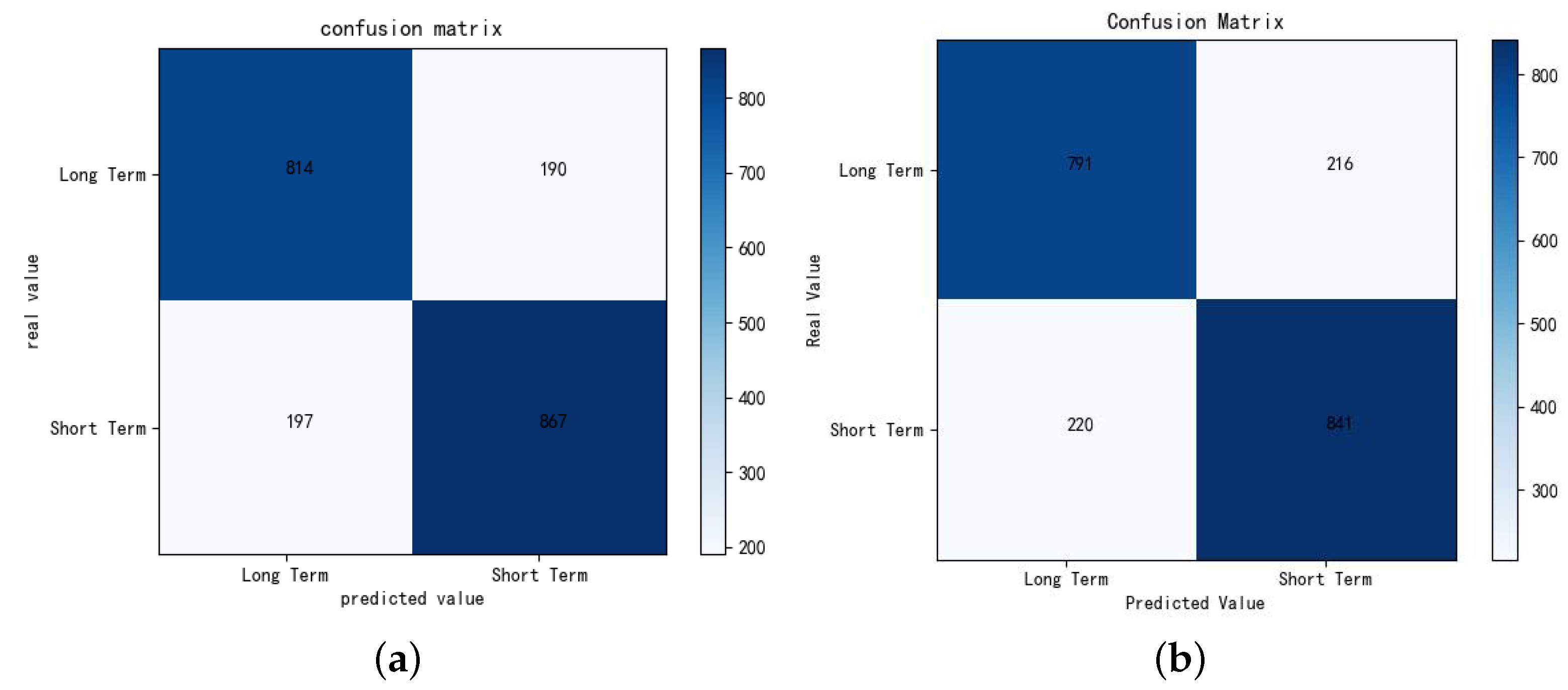
| Precision | Recall | Accuracy | F1 | |
|---|---|---|---|---|
| DSGD | 0.805 | 0.811 | 0.813 | 0.833 |
| Baseline method | 0.782 | 0.786 | 0.789 | 0.784 |
Disclaimer/Publisher’s Note: The statements, opinions and data contained in all publications are solely those of the individual author(s) and contributor(s) and not of MDPI and/or the editor(s). MDPI and/or the editor(s) disclaim responsibility for any injury to people or property resulting from any ideas, methods, instructions or products referred to in the content. |
© 2023 by the authors. Licensee MDPI, Basel, Switzerland. This article is an open access article distributed under the terms and conditions of the Creative Commons Attribution (CC BY) license (https://creativecommons.org/licenses/by/4.0/).
Share and Cite
Liu, J.; Xu, H.; Deng, X.; Liu, H.; Li, D. A Location-Based Crowdsensing Incentive Mechanism Based on Ensemble Learning and Prospect Theory. Mathematics 2023, 11, 3590. https://doi.org/10.3390/math11163590
Liu J, Xu H, Deng X, Liu H, Li D. A Location-Based Crowdsensing Incentive Mechanism Based on Ensemble Learning and Prospect Theory. Mathematics. 2023; 11(16):3590. https://doi.org/10.3390/math11163590
Chicago/Turabian StyleLiu, Jiaqi, Hucheng Xu, Xiaoheng Deng, Hui Liu, and Deng Li. 2023. "A Location-Based Crowdsensing Incentive Mechanism Based on Ensemble Learning and Prospect Theory" Mathematics 11, no. 16: 3590. https://doi.org/10.3390/math11163590