Abstract
The accurate classification of seizure types using electroencephalography (EEG) signals plays a vital role in determining a precise treatment plan and therapy for epilepsy patients. Among the available deep network models, Convolutional Neural Networks (CNNs) are the most widely adopted models for learning and representing EEG signals. However, typical CNNs have high computational complexity, leading to overfitting problems. This paper proposes the design of two effective, lightweight deep network models; the 1D multiscale neural network (1D-MSCNet) model and the Long Short-term Memory (LSTM)-based compact CNN (EEG-LSTMNet) model. The 1D-MSCNet model comprises three modules: a spectral–temporal convolution module, a spatial convolution module, and a classification module. It extracts features from input EEG trials at multiple frequency/time ranges, identifying relationships between the spatial distribution of their channels. The EEG-LSTMNet model includes three convolutional layers, namely temporal, depthwise, and separable layers, a single LSTM layer, and two fully connected classification layers to extract discriminative EEG feature representations. Both models have been applied to the same EEG trials collected from the Temple University Hospital (TUH) database. Results revealed F1-score values of 96.9% and 98.4% for the 1D-MSCNet and EEG-LSTMNet, respectively. Based on the demonstrated outcomes, both models outperform related state-of-the-art methods due to their architectures’ adoption of 1D modules and layers that reduce the computational effort needed, solve the overfitting problem, and enhance classification efficiency. Hence, both models could be valuable additions for neurologists to help them decide upon precise treatments and drugs for patients depending on their type of seizure.
Keywords:
deep learning; epileptic seizure; MSCNet; EEG-LSTMNet; spectral–temporal; spatial convolution; depthwise layer; separable layer; TUH database; LSTM MSC:
68T07
1. Introduction
Epilepsy is a prevalent chronic neural disorder resulting from irregular electrical discharges affecting the brain and how it functions, which are known as epileptic seizures. These seizures caused by frequent and unexpected abnormal brain reactions occur as a response to the abnormal electrical discharges generated via neurons [1,2]. The main symptoms of seizures are serious injuries, convulsions, the loss of awareness, changes in behavior or emotions, the uncontrollable movements of arms and legs, temporary confusion, and death in some cases [3].
Epileptic seizures occur spontaneously and are frequently recurrent. They vary in duration and severity, and the symptoms a patient experiences are mainly based on the type of seizure [4,5]. Hence, to decide the correct and precise treatment for an epilepsy patient, there is a need to find out the exact epileptic seizure type they suffer from [6]. In other words, detecting the accurate seizure type can effectively assist neurosurgeons in recognizing the brain cortical connectivity, acquiring information concerning the potential triggers of seizures, and identifying the risk of different expected consequences, intelligence debility, learning difficulties, and sudden death [7,8]. There are three basic classes of epileptic seizures: focal, generalized, and unknown. Each class is defined based on when and how a seizure begins in the patient’s brain. The first class, focal seizures, begins in one area or a group of cells on the same brain side. They are categorized into simple and complex partial seizures. The second class, generalized seizures, begins instantaneously in groups of cells on both brain sides. They are classified into myoclonic, clonic, tonic, and tonic–clonic seizures. The final class, unknown seizures, has unknown beginnings [9,10].
Around 80% of epileptic seizures can be effectively managed when properly and diagnosed in a timely manner [11]. The diagnosis of epilepsy depends on performing a complete medical evaluation, including a physical assessment, neurological assessment, and some brain imaging tests, such as a Computerized Tomography (CT) scan or Magnetic Resonance Imaging (MRI). The Electroencephalogram (EEG) remains the most widely adopted technique for diagnosing and understanding epilepsy. It is used to record the brain’s electrical activity and recognize the type of seizures a patient is experiencing. Some automated seizure classification methods have been developed to detect epileptic seizures, such as deep learning and machine learning [12]. Among these methods, deep learning ones mimic the brain’s learning process and learn helpful representations from EEG data with no need to apply data transformation stages [13].
The most commonly used deep learning architectures to capture patterns during seizures are CNNs [14,15]. In CNNs, different layers are trained using modern methodologies, which makes them significant and broadly adopted deep learning methods. A typical CNN comprises three distinct layers: convolution, pooling, and fully connected [16]. The most commonly used models in the literature for categorizing seizures are 2D CNN-based methods. These models require a large amount of computational effort and are subject to overfitting due to the significant difference between the small number of EEG trials and the large number of output learnable parameters [17,18]. We propose two 1D deep network models, the 1D-MSCNet model and the EEG-LSTMNet model, as efficient, lightweight, and expressive deep network models. The two models aim to classify epileptic seizure types, avoid the high computational complexity of previous models, and solve the overfitting problem, based on achieving a balance between the number of input instances and learnable parameters. The contributions of this paper are as follows:
- Two 1D deep network models, the 1D-MSCNet and the EEG-LSTMNet, are proposed to classify seizure types with low computational effort due to the 1D structures included. The 1D-MSCNet involves separable convolution layers, which break down a 2D convolution operation into two separate 1D convolutions, while the EEG-LSTMNet model adopts both depthwise and separable convolution layers.
- The two models are designed to balance the difference between the input EEG trials and the learnable parameters. While the 1D-MSCNet model applies temporal convolutional layers with separable layers, the EEG-LSTMNet model applies depthwise convolutional layers, separable convolution layers, and LSTM layers to reduce the number of learnable parameters.
- An LSTM module is incorporated into the EEG-LSTMNet model to encode long-term dependencies between time series.
- As a solution to the overfitting problem, the Synthetic Minority Oversampling Technique (SMOTE) algorithm is used. It creates a balance among the training data by raising the number of trials in the minority classes.
The residual sections of this paper are arranged along these lines: Section 2 includes a review of methods related to the field of the paper. Section 3 introduces the proposed 1D-MSCNet and EEG-LSTMNet models, details the models’ formulation, and discusses their architectures. Section 4 proposes the network training process of both models. Section 5 describes the evaluation protocol applied and measured metrics for both models and introduces the used dataset. Section 6 explores the experiments conducted on both models, discusses the obtained results, and shows a comparison between both models. The EEG-LSTMNet model performance is analyzed in Section 7 by examining the use of the confusion matrix and t-SNE plots, the representation of the SHAP plots, and topo maps to indicate the contribution and effect of input channels. A comparison between the proposed and published models is presented in Section 8. Section 9 describes the models and outcomes obtained. The paper is summarized in Section 10. A comparison of the proposed models with cutting-edge models can be found in Section 8. The models and findings are discussed in Section 9. The paper is summed up in Section 10.
2. Related Works
The automatic classification of seizure types from EEG signals allows physicians to obtain a more accurate diagnosis and efficiently manage the disease. Therefore, different methods have been proposed to identify the types of epileptic seizures from EEG trials using deep learning models. A review of these methods is introduced in this section.
The multiscale neural network comprises multiple-scale feature extraction layers and constructs a deep architecture. Moreover, it has a low-rank convolution kernel equal to the input channels. It allows typical networks to classify data more effectively. Multiscale neural network models have been proposed in the literature to extract feature representations in multiple frequency/time ranges and discover spatial representations for subject identification purposes [18,19,20]. First, in the following paragraphs, we give an overview of the methods that use multiscale information.
Asif et al. [21] presented a SeizureNet that learns multiple spectral feature representations using an ensemble architecture to classify cross-patient seizure types into eight classes. The input EEG signals were selected from 20 channels and preprocessed using the Fourier Transform (FT). The proposed model initially converted raw time-series EEG signals into saliency-encoded spectrograms that were then sampled at various frequencies and spatial resolutions. They were then fed into an ensemble of deep CNNs. The ensemble comprised three sub-networks, where their outputs were combined through summation. The combined outputs were then fed into a SoftMax operation classification module to classify seizure types by generating probabilistic distributions regarding the target classes. The presented model was assessed using the TUH database with 5-fold seizure-wise cross-validation. The ADAM optimizer with a batch size of 50 was applied for the training. Outcomes revealed that the presented model obtained an F1-score of 94%.
Hussein and Ward [22] proposed a multiscale CNN approach to classifying four seizure types using intracranial EEG (iEEG) data. The raw input data from 16 channels were initially preprocessed to reduce the data size, divided into smaller segments, and then encoded into an image-like format. The short-time Fourier transform (STFT) was then used to obtain a 2D representation of each iEEG segment. The images were then fed into a multiscale CNN architecture that combined CNNs, for the same filter size (1, 1). Each model included a parallel path to adopt maximum pooling and convolution operations. The outputs from the parallel paths were concatenated into a single feature vector to be flattened and fed into two fully connected layers. They were connected to a sigmoid function to calculate the label probabilities and predictions. The presented model was evaluated using iEEG data from the 2016 Kaggle seizure prediction competition. The results revealed an average sensitivity of 87.85%.
Gao et al. [23] proposed a temporal–spatial multiscale CNN framework with dilated convolutions to determine seizure from non-seizure signals based on capturing the multiscale features of input EEG signals. The input raw EEG signals from 18 channels were preprocessed in two stages to extract their features: the temporal multiscale and spatial multiscale. In each stage, the multiscale features of the EEG signals were extracted along the related dimension with different convolutional kernel sizes. In the temporal multiscale stage, convolution kernels with small sizes focused on local information, while large ones focused on long-term temporal information. A max-pooling layer was added after the convolutional layer to reduce the dimension of the features. Following this, a multiscale spatial stage considered the specific multiscale relations between EEG channels. Next, a dilated convolution was adopted and fed with these features to expand the respective fields of the model. Finally, the vector was fed into a fully connected layer. It was connected to the sigmoid activation function. The proposed model was evaluated using the CHB-MIT dataset with the 5-fold cross-validation method. The results revealed an average sensitivity of 93.3%.
Wang et al. [24] proposed a multiscale dilated 3D CNN to classify four types of epileptic seizures. The model was based on analyzing the time, frequency, and channel information of EEG signals using the STFT. It adopted 3D kernels to simplify the extraction of features over the 3D CNN. The proposed dilated 3D CNN structure comprised three convolutional layers, three max-pooling layers, a single global average pooling layer, and a single fully connected layer. Each convolutional layer included four blocks with different dilated sizes. Each block’s outputs were combined after the final layer to be fed into the global average pooling layer to reduce the number of parameters. The fully connected layer was combined with a SoftMax function that computes the probabilities of classes. The performance was assessed using the CHB-MIT EEG database with a leave-one-out cross-validation method. The results revealed that the proposed model achieved 80.5% accuracy.
Some methods have used single-scale deep models. The EEGNet is a CNN-based compact network adopted in BCIs. It combines depthwise convolution and separable convolution, which capture the temporal and spatial filters as a substitution for the typical square convolution, reducing the number of parameters. However, the application of the EEGNet model to classify seizure types is limited in the literature, and there is only one available research study model by Peng et al. [25]. The model was composed of three blocks. The first block included two sequential convolutional layers. The first layer captured the feature maps of input EEG signals from 20 channels, while the second layer executed a depthwise convolution. To improve the temporal information, a TIE module was augmented to the convolutional layer to construct a TIE-Conv2D layer. The outputs were then fed into the second block that included separable convolution along with a depth-wise convolutional layer and a subsequent point-wise convolutional layer. This block ensured that the number of parameters was decreased and that the relations within and across feature maps were obtained in a decoupled way. The final block was the classification, which included a fully connected layer with SoftMax activation. The model performance was evaluated using two databases; TUSZ and CHSZ with a 3-fold cross-validation. The results revealed that the proposed model efficiently classified cross-subject seizure types with 67.2% accuracy.
It is obvious from the reviewed works that efficient results have been obtained for categorizing various types of seizures using multiscale and single-scale CNN models. However, the existing multiscale neural network models mostly suffer from a high computational complexity, leading to overfitting problems due to their complex structures. The method based on the single-scale EEGNet model also revealed a low classification accuracy result. Therefore, the aim of this paper was to solve the challenges of those models by proposing two effective, lightweight, and expressive deep network models, the 1D-MSCNet model and the EEG-LSTMNet model, to accurately classify seizure types using EEG trials collected from the TUH database with the lowest possible computational efforts needed and the highest reduction in the number of output learnable parameters achieved.
3. Proposed Method
This work aims to categorize epileptic seizure types using EEG data. Thus, the problem is initially formulated for the 1D-MSCNet and EEG-LSTMNet models. Next, the details of the two models are explored.
3.1. Problem Formulation
Both the 1D-MSCNet model and the EEG-LSTMNet model are trained and tested using the same EEG trails gathered from the TUH dataset. The EEG trial is deployed to recognize the seizure type, where it is signified as a matrix . C represents the number of channels in this matrix, whereas T represents the number of time stamps:
where C1, C2, ……Cr are the channels of EEG trials, which are collected from several sites on the scalp, and ci (tj) represents the captured potential at time tj. denotes the space of those EEG trials. The seizure class is identified using class labels Y= {AB, CP, FN, GN, SP, TN, TC, and MY}, where AB, TN, TC, CP, FN, GN, SP, and MY represent the seizure types, namely absence, tonic, tonic colic, complex partial, focal non-specific, generalized non-specific, simple partial, and myoclonic, respectively. The function that associates an EEG trial to a label ca be expressed as:
F is designed in this work using the two CNN models. Input EEG trials are first preprocessed for both models by resampling them into 250 Hz. Then, the SMOTE algorithm [26], an efficient oversampling method, is used to overcome the data imbalance problem. It randomly increases the minority class instances in the training set based on duplicating them and then producing new minority instances among the available minority instances. The only parameter for SMOTE is the number of nearest neighbors; we used the default number of nearest neighbors, which is five.
3.2. 1D-MSCNet Model
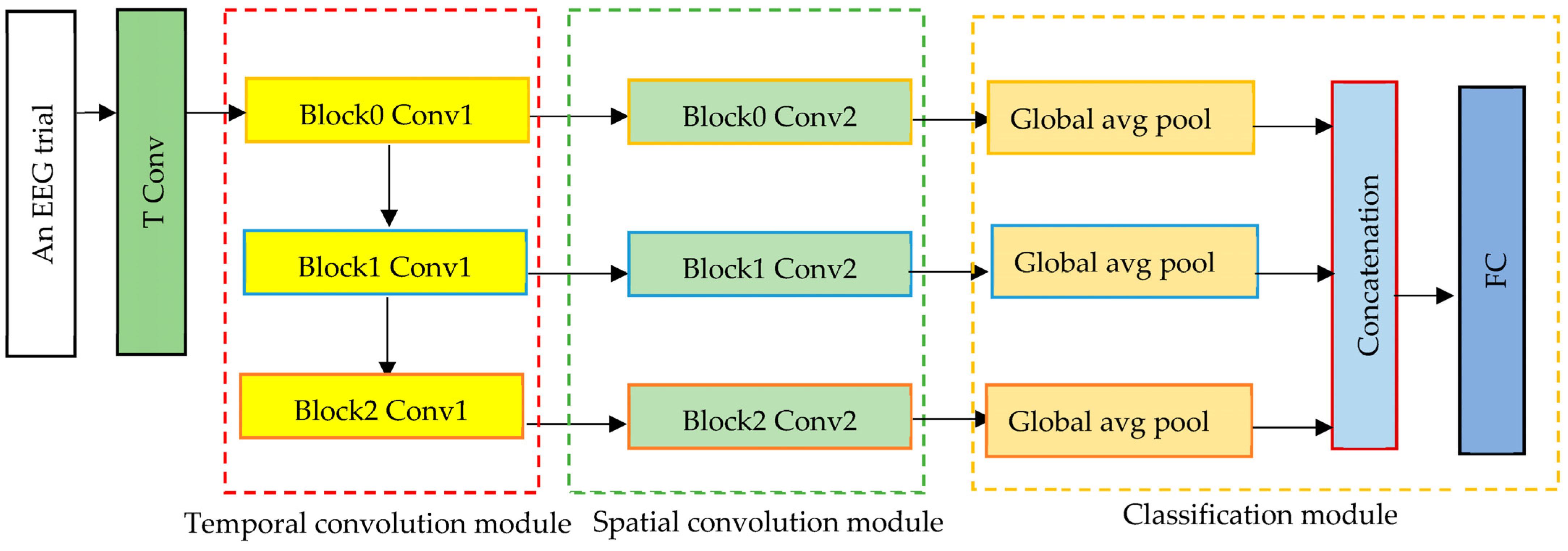
The proposed 1D-MSCNet neural network model learns multiscale features automatically from data using multiple spectral filters. It comprises three modules: a separable temporal convolution module, a spatial convolution module, and a classification module, as represented in Figure 1. Each module’s architecture is described in the following paragraphs.
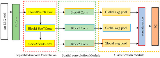
Figure 1.
The proposed 1D-MSCNet model comprises a separable temporal convolution module, a spatial convolution module, and a classification module.
Based on Figure 1, the input trials are initially processed via a temporal convolutional (TConv) layer that extracts the temporal features. EEG signals are input channel-wise into a temporal convolutional layer to enhance the number of feature maps. The activated features have the form , where , in which both stands for the sampling frequency and denotes the feature map dimension of the first temporal convolution layer. This layer converts input EEG trials into temporal feature maps in the separable temporal convolution module.
- Separable Temporal Convolution Module
It comprises three separable temporal convolution layers, as shown in Figure 1. Each separable convolution layer breaks down into two separate convolutions: depthwise temporal convolution and point-wise convolution. The principal advantages of utilizing separable convolutions are the significant reduction in the adjustable weights and the efficient separation of the temporal and spatial dimensions. To do this, kernels are individually trained for each feature map. This layer ensures a decrease in the number of learnable parameters. The proposed multiscale neural network model utilizes intermediate activations to discover multiscale characteristics from input data. Consequently, the suggested model acquires N spectral temporal features. as expressed below:
where denotes the k-th separable convolution, denotes the first temporal convolution and denotes the function composition among arbitrary functions and , where .
Consequently, by determining the features , , …, , the multiscale neural network effectively learns the multiscale spectral–temporal features. A spatial convolution module with different kernel sizes follows the spectral–temporal convolution module. It convolves various spectral–temporal features in a filter-independent way.
- Spatial Convolution Module
It consists of three spatial convolution blocks used to extract spatial information from the EEG channel distributions of the retrieved multiscale spectral and temporal representation from the first module. In this module, the kernel size is equivalent to the number of input EEG channels. Thus, it is equal to 21 in this work. From spectral–temporal features, this module derives the spatial characteristics of each range. In contrast to conventional CNNs, the proposed model employs each intermediate active feature set to collect spatial information, enabling the extraction of several multiscale ranges of EEG characteristics. This module’s output features are then sent to the classification module to categorize seizure types.
- Classification Module
It consists of three layers: global average pooling, a concatenation layer, and a fully connected layer. Each global average pooling layer aggregates the nodes of each feature map to eliminate the requirement for any window size or stride. The output from each spatial convolution layer is then sent to a global average pooling layer within the classification module to identify relevant features and minimize the number of model parameters. This is performed by flattening the feature maps that assist in solving the overfitting and generalization problems. The classifier then concatenates the output features from the global average pooling layers in the feature map dimension, where the concatenated feature can be expressed as follows:
where N is the number of sizes of the spatial-spectral–temporal features , and is the concatenation operation. The concatenated features are then forwarded to the eight-neuron fully connected layer. Each neuron is relative to one seizure class. This layer adopts the SoftMax function, which turns a vector of N real values into a vector of N real values that sum to 1. The SoftMax function calculates the probability of each class to determine the class of input trials.
3.3. EEG-LSTMNet Model
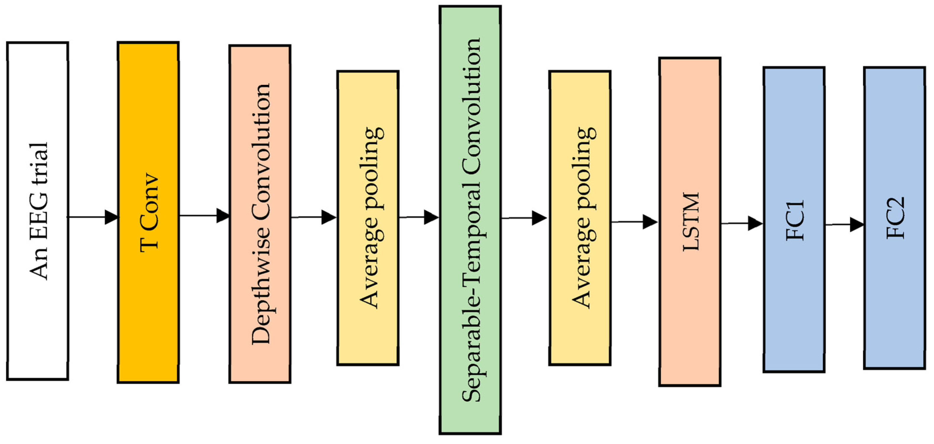
The proposed EEG-LSTMNet model can be efficiently applied across various BCI paradigms; it can be trained using very limited data and can also extract neuro-physiologically interpretable features from input data. The model consists of three types of convolutional layers, namely temporal convolution, depthwise convolution, and separable convolution, in addition to two average pooling layers, an LSTM layer, and two fully connected classification layers, as shown in Figure 2. The bias units are omitted in all the convolutional layers within the model. A description of these layers is presented in the next paragraphs.
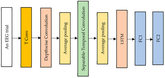
Figure 2.
The architecture of the proposed EEG-LSTMNet model.
- Temporal Convolution Layer
This involves extracting temporal features from input EEG trials with a filter size equal to half of the sampling rate. Therefore, it is employed in the proposed model to transform the input EEG samples into a collection of temporal feature maps that are then sent to the depthwise convolution layer.
- Depthwise Convolution Layer
This is a convolution layer with a single convolutional filter for each input channel. Adopting the depthwise convolution layer is primarily intended to reduce the number of learnable parameters and prevent the overfitting issue. It also reduces the computation needed in convolutional operations while enhancing representational efficiency. Additionally, this layer determines spatial filters for each temporal filter, efficiently extracting frequency-specific spatial representation. After applying the ReLu nonlinearity [27], batch normalization and feature map dimension techniques are used. The output features from this layer are then fed into an average pooling layer.
- First Average Pooling Layer
This is a pooling operation of size two that is applied after the convolutional layers in order to compute the average value of the patches of the feature map, which is then used to create a down-sampled (pooled) feature map. The outcome from this layer is passed to the third convolutional layer.
- Separable Temporal Convolution Layer
This decomposes a convolution layer into two convolution layers (depthwise temporal and point-wise convolution layers) to obtain the same result with reduced computing effort. Consequently, this layer reduces the number of learnable parameters and decouples the relations within and across feature maps by learning a kernel that summarizes each feature map separately and then combines the results. In addition, it divides learning how to summarize individual feature maps over time and learning how to integrate these feature maps. The output of this layer is subsequently sent to a second average pooling layer.
- Second Average Pooling Layer
This is a layer of size two that is applied after the separable convolution layer to reduce the dimensionality. The layer’s output is subsequently sent to the LSTM layer.
- LSTM Layer
In CNNs, this layer is used to transition from the convolution layer to the fully connected layer. It overcomes the problem of vanishing gradients in conventional neural networks by introducing extra gates to learn longer-term relationships in sequential input. This enables it to manage the data within the hidden cell that must be delivered to the subsequent hidden state. In addition, it incorporates a constant error backpropagation flow within its memory cells to bridge temporal periods greater than 1000 time steps. To properly encode the time series characteristics of each EEG trial input into the proposed EEG-LSTMNet model by learning and fusing the long-term dependencies in the data together with the critical temporal properties, the LSTM layer is utilized in the proposed EEG-LSTMNet model. The output of the LSTM layer is subsequently sent to the classification layers.
- Classification Layers
There are two classification layers. The first layer is a time-distributed dense layer, which accepts a batch size according to the sequence length of the input size array and creates a batch size according to the sequence length of the size array for the number of classes. It is applied in the proposed EEG-LSTMNet to decrease the LSTM output dimension. The output of the first layer is passed to the second layer, which comprises eight neurons. Each neuron is relative to one seizure class. This layer is connected to a SoftMax function, which converts a vector of N real values into a vector of N real values with a summation of 1. Consequently, the SoftMax function in this study provides the class probability of each class, which is used to identify the input class.
4. Training the Network
Both the models’ input EEG trials acquired from the TUH dataset are initially divided into a stratified 80% training set and 20% validation and testing sets based on patients. Next, the 20% is divided into 10% for validation and 10% for testing sets. We split the data randomly based on the patients so that the patients included in the training dataset and validation datasets are not present in the testing set. The training set learns the model’s learnable parameters. The validation set manages the training process. The Google Cloud Platform is used to execute the model training process, where the learning rate is dependent on the number of epochs, as shown below:
- For epoch > 40, the learning rate is increased by 1 × 10⁻¹
- For epoch > 80, the learning rate is increased by 5 × 10⁻²
- For epoch > 130, the learning rate is increased by 2.5 × 10⁻³
- For epoch > 150, the learning rate is increased by 5 × 10⁻⁴
For both models, the total number of epochs is 190 for a batch size of 128. Moreover, both models are fitted using the Adam optimizer based on updating their weights with the training dataset. The testing dataset is then utilized to assess the categorization results of both models. To avoid the problem of overfitting, the L2 Regularization approach is utilized. The SMOTE algorithm is solely applied to the training data to enhance the number of training trials.
5. Protocol for Evaluation
To assess the efficacy and performance of both models, 1D-MSCNet and EEG-LSTMNet, in classifying the seizure type from EEG trials, the models were trained and evaluated using the TUH dataset. This section provides an overview of the TUH dataset. In addition, it covers the assessment technique and evaluates the performance of the trained models using evaluation metrics.
5.1. Dataset
The TUH EEG seizure corpus dataset includes clinical data acquired at Temple University Hospital (TUH) from 2001 until now as a support to research focused on interpreting EEG signals via machine learning algorithms [28,29]. Outpatient services, the intensive care unit (ICU), the epilepsy monitoring unit (EMU), and the emergency department were among the hospital sectors from which data were collected (ER). The international 10/20 system was used to standardize the placement of 21 scalp electrodes for EEG signal recording. The distance between each pair of electrodes in the system is 10 to 20 percent of the distance between the nasion (in the front) and the inion (in the rear) (in the back) [30].
In this work, the TUH dataset version 1.5.2, which circulated in 2022, is adopted. It is the largest available dataset of seizure and non-seizure data. For all conducted experiments, 21 channels are considered, including FP1, FP2, F3, F4, C3, C4, P3, P4, F7, F8, T3, T4, T5, T6, O1, O2, A1, A2, FZ, CZ, and PZ. In the dataset, there are 5612 EEG trials from 642 patients, of whom 242 experience seizures. In total, 5612 of the data files are seizure files, whereas the remaining files are non-seizure files; these were disregarded because this study focused solely on seizures. There are eight seizure types within the dataset, including absence (AB), tonic (TN), tonic colic (TC), complex partial (CP), focal non-specific (FN), generalized non-specific (GN), simple partial (SP) and myoclonic (MY) seizures. The number of files for each seizure type is shown in Table 1. The sampling rate range varies between 250 Hz and 512 Hz.

Table 1.
Total number of seizure files and the total number of trials in each class [31].
5.2. Evaluation Procedure
The TUH dataset is adopted in this paper for the evaluation process. It is utilized for learning and validating both models in the conducted experiments. The EEG signals available in the TUH dataset were captured with different sampling rates. The EEG signals are first preprocessed to obtain normalized data. This is based on resampling the data to 250 Hz since 87% of them were recorded at the sampling rate of 250 Hz. Each EEG signal is then divided into trials using a fixed 2 s window and 0.5 s stride. Thus, there are sufficient trials to learn the model and solve the overfitting.
We split the data randomly based on patients so that the patients included in the training data and validation datasets are not present in the testing set. The TUH dataset is firstly stratified and segmented into an 80% training set and 20% validation and testing sets using a train test split. Next, the 20% is divided into 10% for the validation set and 10% for the testing set. Eighty percent of the data are then augmented using the SMOTE algorithm. It augments the training dataset such that the minority classes, primarily AB, TN, TC, and MY, are represented proportionally. It is based on increasing the number of trials to 500,000.
5.3. Evaluation Metrics
The performance of the 1D-MSCNet and the EEG-LSTMNet models can be assessed using various evaluation metrics. The adopted metric in this paper is the F1 score. It is an essential machine learning metric that computes the model’s accuracy based on combining its precision and recall scores. In contrast to accuracy, which focuses on accurately classifying positive and negative observations, the F1-score balances the precision and recall of the model on the positive class.
Four main measures are computed to measure the F1-score of the model, including True Positives (TP), False Positives (FP), True Negatives (TN), and False Negatives (FN). The TP stands for the number of correctly classified seizure trials. The FN stands for seizure trials that are incorrectly classified as non-seizures. The TN stands for correctly classified non-seizure trials. Lastly, the FP stands for non-seizure trials that are incorrectly classified as seizure trials. The accuracy, precision, recall, and F1-score can be calculated based on the following metrics:
6. Experiments and Results
Different experiments were conducted to assess the effectiveness and evaluate the classification performance of both models; the 1D-MSCNet model and the EEG-LSTMNet model. This section details the experiments performed with each model and discusses the obtained results. It then presents a comparison between the two models.
6.1. Experiments Performed with 1D-MSCNET and the Results
The performance of the 1D-MSCNet model is evaluated by carrying out two experiments. The first experiment concerns the selection of the best modules for the proposed model. In contrast, the second experiment examines the impact of adopting the separable temporal convolution module on the performance of the model.
- Specification of the architecture of the 1D-MSCNET
The architecture of the proposed 1D-MSCNet model comprises three main modules, as shown in Figure 1, including a separable temporal convolution module, a spatial convolution module, and a classification module. The separable temporal convolution module includes three separable temporal convolution layers that extract multiscale spectral–temporal features from input EEG trials using intermediate activations. This module decreases the adjustable weight and decouples the temporal and feature map dimensions of the input features in an efficient manner. Consequently, the number of learnable parameters is decreased.
The output multiscale spectral–temporal representation from the first module is input into the spatial convolution module, which extracts spatial patterns from the multiscale features using a kernel size of 21. The multiscale spatial–spectral–temporal features extracted from each spatial convolution layer are then input into a global average pooling layer inside the classification module to select relevant features and minimize the number of parameters. This is performed by flattening the feature maps, which solves overfitting and generalization problems.
The output features from the global average pooling layers are then concatenated in the feature map dimension and sent to the fully connected layer, which consists of eight neurons specific to eight seizure types. Table 2 illustrates the specification of each module and the number of parameters to be learned. The suggested 1D-MSCNet neural network model efficiently decreases the number of learnable parameters to 469,000 as shown in Table 2, where it revealed an F1-score of 96.9%.
Table 2.
The specification of the architecture of 1D-MSCNet.
- The Impact of Adopting a Separable Temporal Convolution Module
In this experiment, the separable temporal convolution module in 1D-MSCNet is substituted by a temporal convolution module, as shown in Figure 3, to evaluate its impact on the model’s performance. The temporal convolution module includes three temporal convolution layers, whereas the separable temporal convolution module comprises three separable temporal convolution layers; in both cases, the extracted features are multiscale spectral–temporal features because the filter sizes are the same in both cases, i.e., 1 × 31.

Figure 3.
The architecture of the of the second version of the 1D-MSCNet model.
In the second configuration of 1D-MSCNet, the input EEG signals are passed into three temporal convolutional layers of the temporal convolution module to extract multiscale spectral–temporal features. The extracted features from each layer are then passed into the corresponding spatial convolution layer in the spatial convolution module of the model. Similar to the first experiment, the kernel size in the spatial convolution module is 21 × 1, as there are 21 EEG channels. Each layer in this module derives the spatial features of each range from the spectral–temporal features. The output features from the module are then passed to the classification module to classify seizure types.
As in the first experiment, the classification module comprises three global average pooling layers, a concatenation layer, and a fully connected layer. To extract the key features and decrease the number of model parameters, the output of each spatial convolution layer is passed to a corresponding global average pooling layer. This is performed by flattening the feature maps, which helps to reduce overfitting and generalization problems.
The output features from the global average pooling layers are then concatenated by the classifier in the feature map dimension. The concatenated features are then transferred to a fully connected layer of eight neurons, each corresponding to a different class. The SoftMax function is adopted in this layer to turn a vector of N real values into a vector of N class probability values with a summation of 1. Thus, each class’s probability is computed to determine the class of the EEG input trials. Table 3 depicts the specification of the second architecture for each module and the total number of learnable parameters.
Table 3.
Architecture of the second configuration of 1D-MSCNet.
Based on Table 3, the second configuration increases the number of learnable parameters to 549,416 and achieves an F1-score of 94%. Hence, it can be noted that the first configuration shown in Figure 1 achieves a higher F1-score of 96.9% and greatly reduces the number of learnable parameters to 469,000. This establishes that when the separable temporal convolution module is used to extract multiscale features for the classification of the seizure type, the model yields improved classification outcomes with a significant reduction in the number of learnable parameters. This happens because the separable temporal convolution breaks down a temporal convolution into two simpler operations, i.e., depthwise convolution, where filters operate separately on each channel of the input feature map, and point-wise convolution. In this way, from the EEG trials, spectral and temporal features are captured separately; these are relevant to the seizure type. On the other hand, in temporal convolution, each filter operates on all channels of the input feature map, and simultaneously computes the spectral and temporal features.
6.2. Experiments Performed with EEG-LSTMNet
The experiment was performed to evaluate the proposed EEG-LSTMNet model, whose configuration is shown in Figure 2. Table 4 demonstrates the specification of each module, and the total number of learnable parameters. The proposed EEG-LSTMNet model efficiently decreases the total number of learnable parameters to 204,396 and obtains an F1-score of 98.4%, as shown in the table. The significant reduction in the number of learnable parameters is due to the presence of depthwise and separable temporal convolution layers in the model. It has been established in Section 6 that, for the analysis of EEG trials to be able to classify seizure types, the separable temporal convolution layer is more efficient in terms of classification performance and reducing the number of learnable parameters. The important hyper-parameter of a separable temporal convolution layer is the number of filters; we performed experiments with 32 and 64 filters, as described in Table 4, and found that having 64 filters gives the best performance. Another important component of the model is the LSTM layer; we performed experiments with and without the LSTM layer and found that it significantly enhances the performance of the model, where the revealed reduction in the number of learnable parameters can be clearly noticed in Table 4. The reason for the significant improvement is that the LSTM layer encodes the long-term dependencies.
Table 4.
EEG-LSTMNet model Architecture Configuration.
6.3. Comparison between the Two Models
This paper proposed two deep network models: the 1D-MSCNet neural network model and the EEG-LSTMNet model. A comparison between the two models and 1DresNet-LSTM [31] is illustrated in Table 5. The 1DresNet-LSTM model comprises three modules: 1D ResNet, LSTM, and the classification module. ResNet helps to avoid the computational complexity and overfitting issues present in conventional CNNs. The LSTM module encodes long-term relationships in order to circumvent the problem of vanishing gradients. The classification module consists of two fully connected layers. The first layer is a time-distributed dense layer used to reduce the output dimension of the LSTM. The output of the first layer is then fed to the second fully connected layer, which consists of eight neurons; each neuron is related to a class. This layer is connected to the SoftMax function, which provides the probability of each class being utilized in predicting the related class of inputs.
Table 5.
Comparison between the two proposed models, 1D-MSCNet and EEG-LSTMNet, and the model proposed in [31].
According to Table 5, the models utilize 1D modules to lower the computational effort required, unlike 2D CNN models, which are afflicted with a high computational complexity. The 1D modules also tackle the overfitting issue by decreasing the number of learnable parameters and lowering the disparity between the number of input instances and the number of learnable parameters. Moreover, the three models reveal a high reduction in this gap by increasing the number of instances in the minority seizure classes by applying the SMOTE algorithm. A further advantageous addition to the models is the set of average pooling layers introduced after the convolutional layers to reduce the number of learnable parameters.
The EEG-LSTMNet model exceeds the other models in terms of its classification accuracy, as evidenced by its attainment of the highest F1-score, namely 98.4%, and a decrease in the number of learnable parameters, totaling 204,390. A depthwise convolution layer inside the EEG-LSTMNet model is partly responsible for this. This layer is superior to other convolutions, results in more accurate models, needs fewer learnable parameters, and is computationally cheaper to train and run.
In addition, the EEG-LSTMNet model employs a separable temporal convolution layer that decomposes a temporal convolution into two lightweight layers (i.e., depthwise convolution and point-wise convolution) to provide the same output with a reduced computing effort and fewer learnable parameters. Consequently, it can be observed that the combination of depthwise, separable temporal convolution and LSTM layers results in a more significant reduction in the number of learnable parameters and the computational effort, as well as a remarkable improvement in the model efficiency when compared to the multiscale neural network model that only employs separable temporal convolution layers and the deep network model that employs the ResNet module. To address the vanishing gradient problem, the deep network model described in [31] and the EEG-LSTMNet models incorporate the LSTM layer into their respective designs. The results illustrate that adopting an LSTM layer leads to higher F1-score values than the multiscale neural network model.
The EEG-LSTMNet model combines the benefits of the other two models and outperforms them. It combines the depthwise and separable temporal convolution layers to minimize the computational effort and the number of learnable parameters compared to the multiscale neural network model that solely uses separable temporal convolution layers. The EEG-LSTMNet model improves the classification performance by incorporating an LSTM layer from the deep network model [31] to overcome the vanishing gradient problem.
7. Analysis of the Performance of EEG-LSTMNet
The performance of the EEG-LSTMNet model is analyzed by computing the confusion matrix and t-SNE plot to illustrate the acquired classification findings. Next, SHAP plots and topographical maps are generated to highlight the contribution and effect of each of the 21 channels for each of the eight seizure classes.
7.1. Confusion Matrix
The confusion matrix is also adopted to visualize and summarize the performance of the EEG-LSTMNet network model. Such a matrix represents the confusion among positive classifications (correctly classified) and negative classifications (misclassified). Figure 4 illustrates the classification results obtained for the eight seizure classes using the confusion matrix.
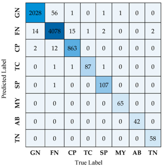
Figure 4.
EEG-LSTMNet confusion matrix.
The confusion matrix shown in Figure 4 demonstrates that 2028 GN seizure trials are accurately labeled as GN, whereas only 14 are incorrectly classified as FN. In contrast, 4078 FN seizure trials are accurately identified as FN, whereas 56 are misclassified as GN. Confusion is present among the FN and GN classes. It is also apparent that there are misclassifications among the CP and FN classes due to the overlap or similarities in their characteristics. Hence, there are similar features or patterns among these classes that cannot be easily distinguished from each other. As seen in Figure 4, classes TC, SP, MY, AB, and TN are always correctly identified with little or no misclassified data.
7.2. Analysis of Network-Learned Representations
A 2D t-SNE plot is used to visualize the discriminability of the features learned by the EEG-LSTMNet network. It visually illustrates the distribution of features corresponding to the eight classes, as seen in Figure 5. Classes TC, SP, MY, AB, and TN have distinct and clustered sample distributions, as shown in Figure 5. On the other hand, some trials from classes CP, GN, and FN are misclassified. According to the confusion matrix, this is mostly due to their overlapping features and comparable qualities.
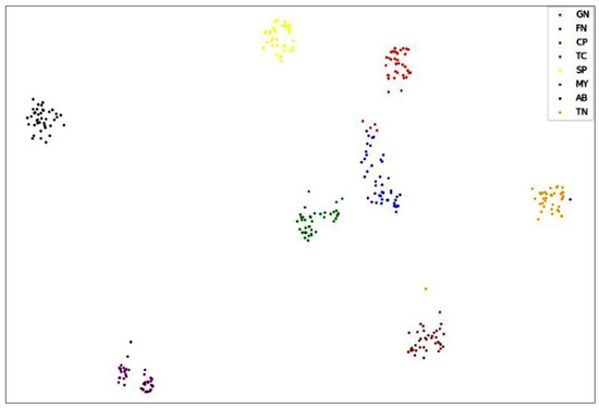
Figure 5.
Visualization of features using the 2D t-SNE plot.
7.3. Visualization of the EEG-LSTMNet Model’s Decision-Making Procedure
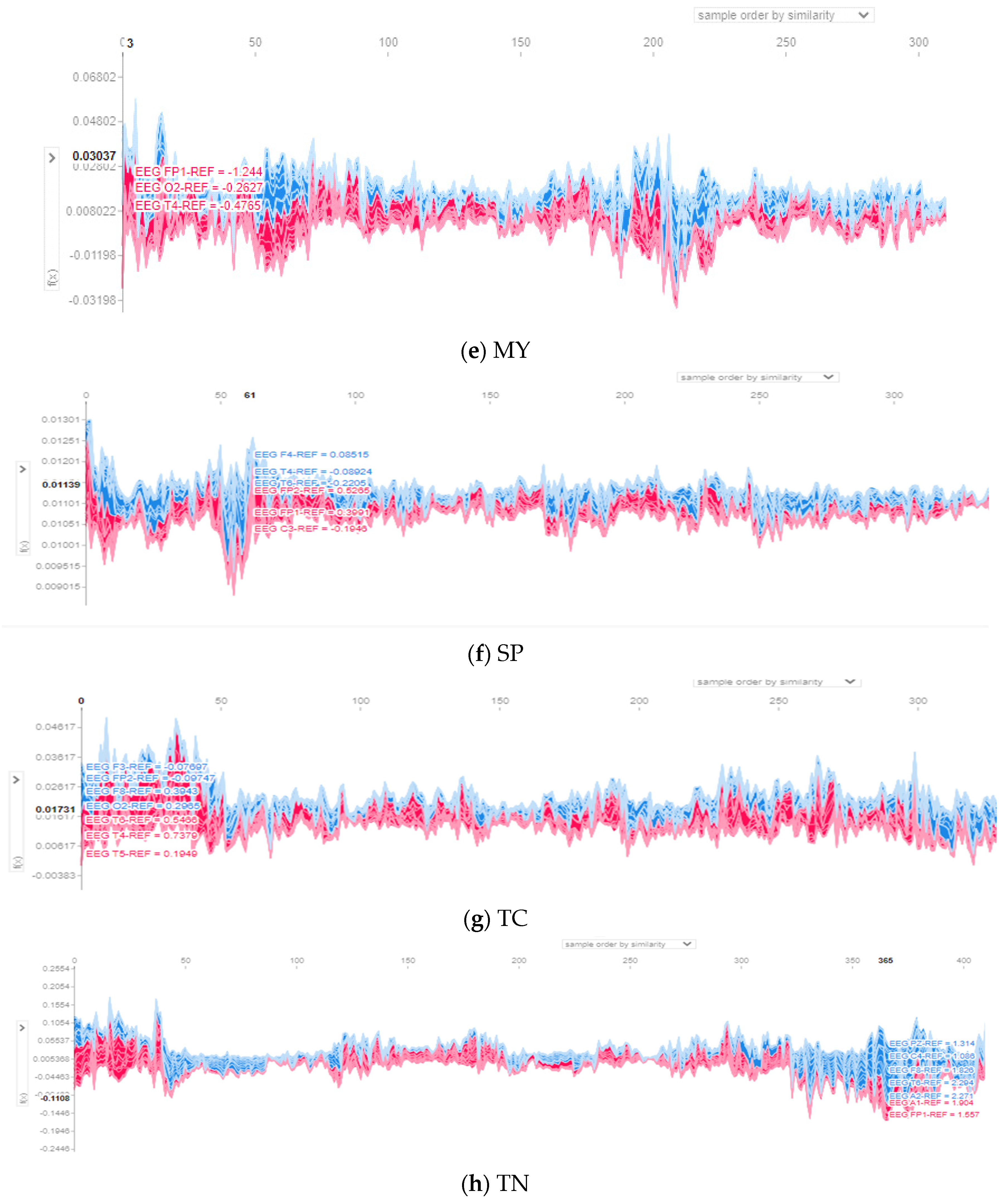
The EEG-LSTMNet model, like any CNN model, is a black box; it is hard to figure out how it classifies the data. Hence, the SHAP (SHapley Additive exPlanations) explainer is adopted to describe the model’s decision-making mechanism. It determines the Shaple values of the input channels. It uses them to calculate the contribution of each channel to the model output to discover the most effective channels on the output. The values and the channels, which effectively contribute to the model prediction for a single observation, are represented using SHAP force plots. Figure 6 depicts the channels that positively or negatively impact the decision-making procedure of the EEG-LSTMNet model for each class. The red part of each graph denotes the channels positively impacting the prediction. In contrast, the blue part of each graph denotes the channels negatively affecting the prediction. The input instances organized according to similarity are plotted on the X-axis, while the model output prediction values are plotted on the Y-axis.
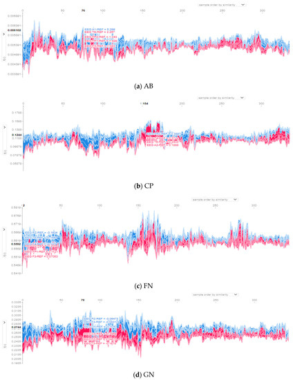
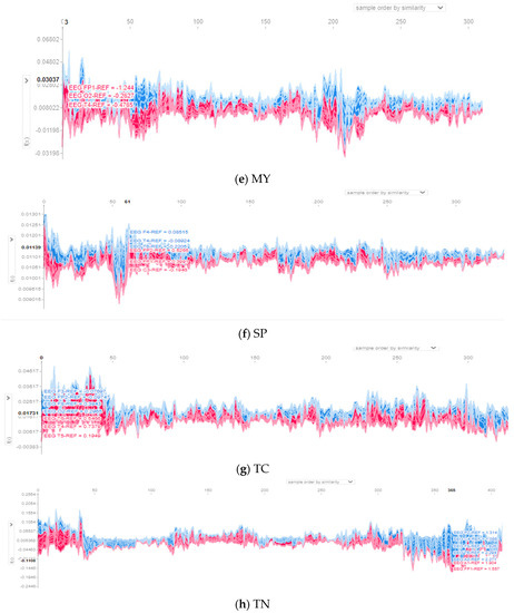
Figure 6.
Contributions of input channels from force SHAP plots for the eight classes: (a) AB, (b) CP, (c) FN, (d) GN, (e) MY, (f) SP, (g) TC, and (h) TN.
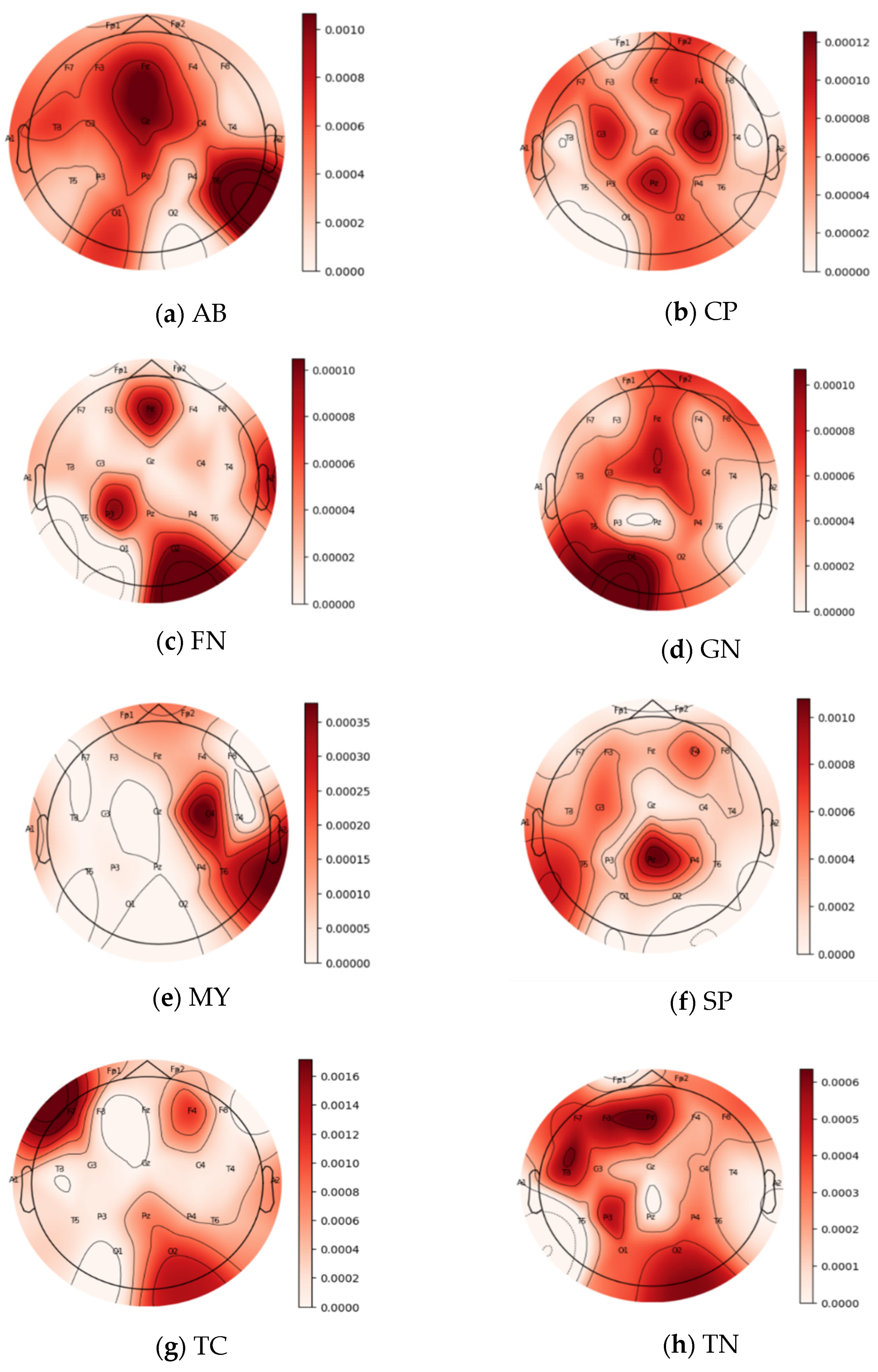
The force plots shown in Figure 6 are consistent with the topo maps of the input 21 channels (FP1, FP2, F3, F4, C3, C4, P3, P4, F7, F8, T3, T4, T5, T6, O1, O2, A1, A2, FZ, CZ, and PZ) for each class. Notably, the letter F stands for the frontal, C for the central, T for the temporal, P for the parietal, and O for the occipital regions. Additionally, the odd numbers inside the channel names represent the brain’s left hemisphere, and the even numbers represent the right hemisphere; Z represents the central channels.
Topo (topographic) maps, or contribution maps, translate the contribution amplitudes into colors, with darker red colors corresponding to greater channel contributions. Figure 6 and Figure 7 depict each seizure class’s force plots and topo maps, respectively.
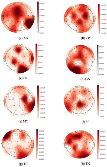
Figure 7.
Contributions of input channels from the topo maps for the eight classes: (a) AB, (b) CP, (c) FN, (d) GN, (e) MY, (f) SP, (g) TC, and (h) TN.
For class AB, contributions are almost spread over all channels, specifically channels T6, FZ, PZ, O1, F3, C3, and T3, as shown in Figure 6a and Figure 7a, with a magnitude of contribution from 0.004 to 0.006. For class CP, illustrated in Figure 6b and Figure 7b, channels C4, PZ, C3, O2, FP2, F7, F2, and F4 positively influence the prediction of this class. These channels’ contribution magnitudes range from 0.06 to 0.18. For the class FN, seen in Figure 6c and Figure 7c, contributions are divided over channels O2, P3, FZ, and A2, suggesting a contribution size between 0.54 and 0.58. For the class GN, depicted in Figure 6d and Figure 7d, the channels with the most significant contribution magnitude are O1, T5, FZ, C3, and FP2, ranging from 0.2 to 0.33.
The contribution in the class MY concentrates on three channels, namely C4, T6, and A2, as illustrated in Figure 6e and Figure 7e. The contribution magnitude revealed is in the range of −0.03–0.06. For class SP, channels PZ, T5, and F4 are the most effective, as illustrated in Figure 6f, with a contribution magnitude range of 0.009–0.013. This is evident on the topo map of the class depicted in Figure 7f.
Figure 6g and Figure 7g of class TC reveal that the effective channels are F1, F4, PZ, and O2, with a contribution magnitude range of 0.004-0.04. Finally, almost all channels have positive effects on class TN, as illustrated in Figure 6h and Figure 7h; these channels are mainly FZ, F3, F7, T3, P3, O1, and O2, with contribution magnitudes ranging from −0.24 to 0.255.
8. Comparison with State-of-the-Art Methods
Table 6 below compares the proposed 1D-MSCNet neural network model with some state-of-the-art models.
Table 6.
Comparison with the state-of-the-art multiscale neuralnetwork-based seizure type classification models.
Table 6 demonstrates that several datasets are used to assess multiscale neural networks models, including the 2016 Kaggle seizure prediction competition in [22], CHB-MIT in [23,24], TUH in [21], and the proposed model. Two core activation functions are used to classify the data within the classification modules of the models, including the SoftMax function in [21,24] and our proposed model, and the Sigmoid function in [22,23]. The proposed model and the state-of-the-art model proposed in [21] classify the data into eight seizure classes using the SoftMax function.
The proposed model achieves the best performance, as revealed by the highest recorded F1-score of 96.9%. This is mainly due to adopting separable convolution layers within the separable, temporal convolution module that breaks down a 2D convolution operation into two separate 1D convolutions. Hence, it requires fewer computations and reduces the risk of overfitting by reducing the number of learnable parameters. Moreover, the classification module within the proposed model adopts three global average pooling layers before the concatenation layer. It offers better performance by reducing the temporal dimensionality of feature maps to obtain a vector for each map.
The performance of the proposed EEG-LSTMNet is compared to that of the state-of-the-art model described in [25], both of which classify eight seizure types. The proposed model in [25] comprises three blocks, block one with temporal and depthwise convolutional layers, block two with a separable, depthwise convolutional layer and a subsequent point-wise convolutional layer, and block three with a single fully connected layer that is connected to a SoftMax activation function. The proposed EEG-LSTMNet outperforms this model in adopting two average pooling layers to compute the average value for the patches of a feature map to create a down-sampled (pooled) feature map. In addition, the proposed deep EEGNet employs an LSTM layer to deal with the problem of vanishing gradients by learning longer-term relationships in sequential data via extra gates.
Unlike the single fully connected classification layer in [25], the proposed EEG-LSTMNet adopts two fully connected layers; the first layer is a time-distributed dense layer, while the second one is connected to a SoftMax function and includes eight neurons. Both models adopt different databases; the suggested EEG-LSTMNet model adopts the TUH database, whereas [25] adopts both the TUSZ and CHSZ databases. The results of both models prove that our model outperforms with a 98.4% F1-score compared with the state-of-the-art model in [25], which achieved 67.2% Accuracy. A comparison between both models is summarized in Table 7 below.
Table 7.
Comparison with the state-of-the-art EEGNet neural-network-based seizure type classification models.
9. Discussion
Considering the outcomes achieved for both models, the 1D-MSCNet model and the EEG-LSTMNet model, it is evident that the two proposed models effectively and accurately classified the eight types of epileptic seizures. Both models exhibited the lowest possible computational efforts needed and solved the overfitting problem between the number of input instances and the learnable parameters. Table 8 provides a summary of the assessment metrics obtained for the categorization of the seizure type using the 1D-MSCNet model. It can be shown that the suggested model obtained an F1-score of 96.9% for identifying EEG trials. The model also reduced the total number of learnable parameters to 469,000.
Table 8.
Performance of the 1D-MSCNet.
The results of the 1D-MSCNet model indicate that incorporating a module for separable and temporal convolution into the model’s design improves its performance. This is because the separable convolution layers within the module reduce the complexity by breaking down a 2D convolution operation into two separate 1D convolutions. Hence, it requires fewer computations and reduces the risk of overfitting. Moreover, by combining the separable temporal convolution and spatial convolution modules, the model has the potential to achieve a better performance by reducing the complexity, improving the computational efficiency, enhancing the feature extraction, and learning greater feature representation. Table 9 summarizes the results for the seizure-type classification using the EEG-LSTMNet model and the effect of different layers in the model; the number of filters represents the number of filters in the separable temporal convolution layer. The model achieved a 98.4% F1-score for classifying EEG trials. The model also reduced the total number of learnable parameters to 204,396.
Table 9.
Effect of different hyper-parameters on the performance of the EEG-LSTMNet.
The proposed model consists of three types of convolutional layers: temporal convolution, depthwise convolution, and separable convolution, in addition to two average pooling layers, an LSTM layer, and two fully connected classification layers. Adopting the depthwise layer reduces the number of learnable parameters, eliminating the overfitting issue. It also reduces the computation needed in convolutional operations while enhancing representational efficiency. In addition, it provides a straightforward method for learning the spatial filters for each temporal filter, enabling the effective extraction of frequency-specific spatial features.
Adopting the separable convolution layer, on the other hand, guarantees the production of 1D separable convolutions to provide the same result with reduced computing effort. By learning a kernel that summarizes each feature map separately and then combining the results, it minimizes the number of learnable parameters and decouples the relations within and across feature maps. The LSTM layer solves the problem of vanishing gradients by utilizing extra gates to discover longer-term relationships in sequential input.
The comparison between the two models indicates that the 1D-MSCNet neural network model recorded the lowest F1-score of 96.9% compared to the EEG-LSTMNet model, which achieved an F1-score of 98.4%. This is because the EEG-LSTMNet model utilized the LSTM module to encode time series, learn long-term relationships, and circumvent the vanishing gradients. It is also revealed that there is a greater reduction in the computational effort needed by the EEG-LSTMNet model due to combining the separable convolution layer with a depthwise convolution layer. This combination reduces both the number of learnable parameters and the computing work required to extract more features. Table 10 presents a comparison between the proposed model and the state-of-the-art model, highlighting the pros and cons of each model.
Table 10.
The pros and cons of the proposed and state-of-the-art-related models.
10. Conclusions
This research proposes building two efficient, lightweight, and expressive deep network models, the 1D-MSCNet model and the EEG-LSTMNet model, to categorize EEG trials from the TUH dataset into eight types of epileptic seizures. Due to the incorporation of 1D structures, both models are designed to categorize seizure types with minimal computing effort and a small number of learnable parameters. The 1D-MSCNet model is designed to automatically train multiscale feature representations from data using multiple discriminative separable filters and to discover the relationships between spatial representations of EEG signals. It comprises three modules: a separable temporal convolution module, a spatial convolution module, and a classification module. The model effectively categorized the eight categories of seizures with an F1-score of 96.9%, bringing the total number of learnable characteristics down to 469,000. The EEG-LSTMNet model is designed to categorize EEG data from diverse BCI paradigms as precisely and efficiently as feasible. There are three convolutional layers in the model: temporal, depthwise, and separable layers, a single LSTM layer, and a classification module. The results showed that the model efficiently classified the eight types of seizures with an F1-score of 98.4% and a reduction in the number of learnable parameters to 204,396.
A comparison between the two models revealed that the EEG-LSTMNet model outperforms the other model in both classification accuracy, measured by the highest revealed F1-score of 98.4%, and the highest reduction in the number of learnable parameters to 204,396. This is due to combining the separable convolution layer with a depthwise convolution layer to obtain a greater reduction in the number of learnable parameters and the computational effort needed. The depthwise layer is strictly superior to other convolutions and results in a more accurate model that needs fewer learnable parameters and is computationally cheaper to train and run. In addition, the model improves the classification performance by employing an LSTM layer to overcome the problem of vanishing gradients. Both lightweight variants can aid neurologists in accurately identifying seizure types. This objective prompted the need for such models to aid neurologists in improving their clinical judgments and controlling therapies for patients based on the type of seizure they suffer from. Further research addressing the mechanisms of the two models will be conducted in the future to improve their efficiency. The performance of the models will be thoroughly evaluated with established clinical guidelines for seizure classification to assess their clinical relevance and potential for enhancing existing diagnostic practices. The practical aspects of implementing the proposed models in clinical settings, such as integration with existing neurology workflows, data privacy concerns, and scalability, need further investigation to make the proposed methods more valuable to practitioners.
Author Contributions
Conceptualization, H.A. and M.H.; Data curation, H.A.; Formal analysis, H.A.; Funding acquisition M.H.; Methodology, H.A. and M.H.; Project administration, M.H.; Resources, M.H.; Software, H.A.; Supervision, M.H.; Validation, H.A.; Visualization, H.A.; Writing—original draft, H.A.; Writing—review and editing, M.H. All authors have read and agreed to the published version of the manuscript.
Funding
The authors extend their appreciation to the Deputyship for Research and Innovation, Ministry of Education in Saudi Arabia for funding this research work through the project no. (IFKSUOR3–482–1).
Data Availability Statement
Public domain datasets were used for experiments.
Conflicts of Interest
The authors declare no conflict of interest.
References
- Yuan, Q.; Zhou, W.; Zhang, L.; Zhang, F.; Xu, F.; Leng, Y.; Wei, D.; Chen, M. Epileptic seizure detection based on imbalanced classification and wavelet packet transform. Seizure 2017, 50, 99–108. [Google Scholar] [CrossRef] [PubMed]
- Raghu, S.; Sriraam, N. Optimal configuration of multilayer perceptron neural network classifier for recognition of intracranial epileptic seizures. Expert. Syst. Appl. 2017, 89, 205–221. [Google Scholar] [CrossRef]
- Lasefr, Z.; Ayyalasomayajula, S.S.V.N.R.; Elleithy, K. Epilepsy seizure detection using EEG signals. In Proceedings of the 2017 IEEE 8th Annual Ubiquitous Computing, Electronics and Mobile Communication Conference (UEMCON), New York, NY, USA, 19–21 October 2017. [Google Scholar]
- Robert, S.; Fisher, J.; Cross, H.; D’souza, C.; French, J.A.; Haut, S.R.; Higurashi, N.; Hirsch, E.; Jansen, F.E.; Lagae, L.; et al. Instruction manual for the ILAE 2017 operational classification of seizure types. Epilepsia 2017, 58, 531–542. [Google Scholar]
- Fisher, S.S.; Acevedo, C.; Arzimanoglou, A.; Bogacz, A.; Cross, J.H.; Elger, C.E.; Engel, J.; Forsgren, L.; French, J.A.; Glynn, M.; et al. ILAE official report: A practical clinical definition of epilepsy. Epilepsia 2014, 55, 475–482. [Google Scholar] [CrossRef]
- Roy, S.; Asif, U.; Tang, J.; Harrer, S. Machine learning for seizure type classification: Setting the benchmark. arXiv 2019. [Google Scholar] [CrossRef]
- Raghu, S.; Sriraam, N.; Temel, Y.; Vasudeva Rao, S.; Kubben, P.L. EEG based multi-class seizure type classification using convolutional neural network and transfer learning. Neural Netw. 2020, 124, 202–212. [Google Scholar]
- Ahmedt-Aristizabal, D.; Fernando, T.; Denman, S.; Petersson, L.; Aburn, M.J.; Fookes, C. Neural memory networks for robust classification of seizure type. arXiv 2019. [Google Scholar] [CrossRef]
- Fisher, R.S.; Cross, J.H.; French, J.A.; Higurashi, N.; Hirsch, E.; Jansen, F.E.; Lagae, L.; Moshé, S.L.; Peltola, J.; Roulet Perez, E.; et al. Operational classification of seizure types by the international league against epilepsy: Position paper of the ilae commission for classification and terminology. Epilepsia 2017, 58, 522–530. [Google Scholar] [CrossRef]
- Scheffer, I.E.; Berkovic, S.; Capovilla, G.; Connolly, M.B.; French, J.; Guilhoto, L.; Hirsch, E.; Jain, S.; Mathern, G.W.; Moshé, S.L.; et al. ILAE classification of the epilepsies: Position paper of the ilae commission for classification and terminology. Epilepsia 2017, 58, 512–521. [Google Scholar] [CrossRef]
- Harvard Health Publications, Harvard Medical School. Available online: www.health.harvard.edu/a_to_z/absence-seizures-petit-mal-seizures-a-to-z (accessed on 18 January 2022).
- Acharya, U.R.; Oh, S.L.; Hagiwara, Y.; Tan, J.H.; Adeli, H. Deep convolutional neural network for the automated detection and diagnosis of seizure using EEG signals. Comput. Biol. Med. 2018, 100, 270–278. [Google Scholar] [CrossRef]
- Zabihi, M.; Kiranyaz, S.; Rad, A.B.; Katsaggelos, A.K.; Gabbouj, M.; Ince, T. Analysis of high-dimensional phase space via Poincaré section for patient-specific seizure detection. IEEE Trans. Neural Syst. Rehabil. Eng. 2016, 24, 386–398. [Google Scholar] [CrossRef] [PubMed]
- Kiral-Kornek, I.; Roy, S.; Harrer, S. Deep Learning Enabled Automatic Abnormal EEG Identification. In Proceedings of the 2018 40th Annual International Conference of the IEEE Engineering in Medicine and Biology Society (EMBC), Honolulu, HI, USA, 18–21 July 2018. [Google Scholar]
- Zhang, Y.; Guo, Y.; Yang, P.; Chen, W.; Lo, B. Epilepsy seizure prediction on eeg using common spatial pattern and convolutional neural network. IEEE J. Biomed. Health Inform. 2019, 24, 465–474. [Google Scholar] [CrossRef] [PubMed]
- Alajanbi, M.; Malerba, D.; Liu, H. Distributed Reduced Convolution Neural Networks. Mesopotamian J. Big Data 2021, 2021, 25–28. [Google Scholar] [CrossRef]
- Saputro, I.R.D.; Patmasari, R.; Hadiyoso, S. Tonic Clonic Seizure Classification Based on EEG Signal Using Artificial Neural Network Metho. SOFTT, 2018, No. 2. Available online: https://openlibrarypublications.telkomuniversity.ac.id/index.php/softt/article/view/8432 (accessed on 1 July 2023).
- Raghu Sriraam, N.; Temel, Y.; Rao, S.V.; Kubben, P.L. A convolutional neural network based framework for classification of seizure types. Int. Conf. IEEE Eng. Med. Biol. Soc. 2019, 2019, 2547–2550. [Google Scholar] [CrossRef]
- Elizar, E.; Zulkifley, M.A.; Muharar, R.; Zaman, M.H.M.; Mustaza, S.M. A Review on Multiscale-Deep-Learning Applications. Sensors 2022, 22, 7384. [Google Scholar] [CrossRef] [PubMed]
- Ko, W.; Jeon, E.; Jeong, S.; Suk, H.-I. Multi-Scale Neural Network for EEG Representation Learning in BCI. IEEE Comput. Intell. Mag. 2021, 16, 31–45. [Google Scholar] [CrossRef]
- Asif, U.; Roy, S.; Tang, J.; Harrer, S. SeizureNet: Multi-Spectral Deep Feature Learning for Seizure Type Classification. arXiv 2020. [Google Scholar] [CrossRef]
- Hussein, R.; Ward, R. Epileptic Seizure Prediction: A Multiscale Convolutional Neural Network Approach. In Proceedings of the 2019 IEEE Global Conference on Signal and Information Processing (GlobalSIP), Ottawa, ON, Canada, 11–14 November 2019. [Google Scholar]
- Gao, Y.; Chen, X.; Liu, A.; Liang, D.; Wu, L.; Qian, R.; Xie, H.; Zhang, Y. Pediatric Seizure Prediction in Scalp EEG Using a Multi-Scale Neural Network With Dilated Convolutions. IEEE J. Transl. Eng. Health Med. 2022, 10, 1–9. [Google Scholar] [CrossRef]
- Wang, Z.; Yang, J.; Sawan, M. A Novel Multiscale Dilated 3D CNN for Epileptic Seizure Prediction. In Proceedings of the 2021 IEEE 3rd International Conference on Artificial Intelligence Circuits and Systems (AICAS), Washington, DC, USA, 6–9 June 2021. [Google Scholar]
- Peng, R.; Zhao, C.; Jiang, J.; Kuang, G.; Cui, Y.; Xu, Y.; Du, H.; Shao, J.; Wu, D. TIE-EEGNet: Temporal Information Enhanced EEGNet for Seizure Subtype Classification. IEEE Trans. Neural Syst. Rehabil. Eng. 2022, 30, 2567–2576. [Google Scholar]
- Chawla, N.V.; Bowyer, K.W.; Hall, L.O.; Kegelmeyer, W.P. Smote: Synthetic minority over-sampling technique. J. Artif. Intell. Res. 2002, 16, 321–357. [Google Scholar] [CrossRef]
- Dyrholm, M.; Christoforou, C.; Parra, L.C. Bilinear discriminant component analysis. J. Mach. Learn. Res. 2007, 8, 1097–1111. [Google Scholar]
- Obeid, I.; Picone, J. The Temple University Hospital EEG Data Corpus Frontiers in Neuroscience. Sect. Neural Technol. 2016, 10, 196. [Google Scholar] [CrossRef]
- Shah, V.; Golmohammadi, M.; Ziyabari, S.; von Weltin, E.; Obeid, I.; Picone, J. Optimizing Channel Selection for Seizure Detection. In Proceedings of the IEEE Signal Processing in Medicine and Biology Symposium 2017, Philadelphia, PA, USA, 2 December 2017; pp. 1–5. [Google Scholar]
- He, K.; Zhang, X.; Ren, S.; Sun, J. Deep residual learning for image recognition. In Proceedings of the 2016 IEEE Conference on Computer Vision and Pattern Recognition (CVPR), Las Vegas, NV, USA, 27–30 June 2016; pp. 770–778. [Google Scholar]
- Alshaya, H.; Hussain, M. EEG Based Classification of Epileptic Seizure Types Using Deep Network Model. Mathematics 2023, 11, 2286. [Google Scholar] [CrossRef]


Disclaimer/Publisher’s Note: The statements, opinions and data contained in all publications are solely those of the individual author(s) and contributor(s) and not of MDPI and/or the editor(s). MDPI and/or the editor(s) disclaim responsibility for any injury to people or property resulting from any ideas, methods, instructions or products referred to in the content. |
© 2023 by the authors. Licensee MDPI, Basel, Switzerland. This article is an open access article distributed under the terms and conditions of the Creative Commons Attribution (CC BY) license (https://creativecommons.org/licenses/by/4.0/).