Article

Macroeconomic Effects of Maritime Transport Costs Shocks: Evidence from the South Korean Economy

Department of International Trade, Jeonbuk National University, Jeonju 54896, Republic of Korea
*
Author to whom correspondence should be addressed.
Mathematics 2023, 11(17), 3668; https://doi.org/10.3390/math11173668
Submission received: 11 July 2023 / Revised: 13 August 2023 / Accepted: 23 August 2023 / Published: 25 August 2023

Abstract

:
In the aftermath of the COVID-19 pandemic, the dramatic increase in maritime transport costs might potentially exert detrimental impacts on the macroeconomy, especially for countries that heavily rely on international trade for their consumption and production activities. Our study employs a small open economy DSGE (Dynamic Stochastic General Equilibrium) model to analyze the impact of maritime transport costs on the South Korean macroeconomy, where maritime transport costs are considered as key factors impacting the law of one price. Positive shocks in maritime transport costs, according to the impulse response function, have positive repercussions on the Consumer Price Index (CPI), terms of trade, nominal exchange rates, and nominal interest rates, but can negatively affect real output and real exchange rate. To verify the validity of the our DSGE model, we utilize a Vector autoregression with exogenous variables (VARX) model to examine the dynamic relationship between maritime transport costs and South Korean macroeconomic variables, based on quarterly data from the first quarter of 2002 to the fourth quarter of 2022. The results of the VARX model coincide with those of the DSGE model. Our findings underline the importance of maritime transport costs in the macroeconomy and hold substantial implications for the considered design and selection of policies to mitigate such shocks.

1. Introduction

Maritime transport, the backbone of global trade, accounts for 80% of the cargo transport volume and 70% of the value transport volume [1]. The occurrence of unforeseen events, such as the global COVID-19 pandemic, the Russo-Ukrainian conflict, and the Suez Canal blockage, has underscored maritime transport’s critical role in global trade. COVID-19-induced public health restrictions have resulted in labor shortages at ports and port congestion, triggering a sharp increase in maritime transport costs [2,3,4]. The subsequent easing of global lockdown measures, divergent recovery rates across nations, and consumption-stimulating policies implemented by various governments have spurred an increase in shipping demand [5]. However, this demand surge has outstripped the available shipping capacity. Furthermore, the escalation of trade imbalances, induced by the COVID-19 pandemic, has plunged the shipping industry into a crisis characterized by container shortages, further constraining the shipping supply capacity [1,5]. Subsequent incidents, namely the blockage of the Suez Canal in 2021 and the Russo-Ukrainian war in 2022, have presented a series of logistical challenges and obstacles to the maritime market. These precipitating events led to a sustained increase in maritime transport costs from the end of 2020 to the end of 2022, consistently setting new records. For instance, the China Containerized Freight Index (CCFI), an indicator of short-term and long-term contract rates, hit a historic high of 3444 points in the first quarter of 2022, approximately four times higher than pre-COVID-19 levels [6,7].
Recently, the drastic fluctuations in the maritime shipping market have sparked serious concerns regarding the relationship between maritime transport costs and domestic economics. As the continuous rise in maritime transport costs will increase the expenses of global supply chains, leading to an increase in the prices of domestic end products in countries dependent on international trade [1,4,7], there is growing concern over how macroeconomic variables interact with changes in maritime transport costs. Compared to other types of economies, the impact of maritime transport costs shocks is generally more pronounced on small open economies that rely on maritime transport [1]. In this context, selecting South Korea as a case study is of particular significance. South Korea’s dependence on maritime transport is especially notable, with over 90% of international goods transportation carried out via sea routes, and the nation’s strategy emphasizes an export-oriented growth model [8]. Therefore, understanding how maritime transport costs affect its domestic macroeconomy is not only vital for South Korea but also offers valuable insights for other small economies that rely on shipping. In summary, the motivation for this study is to explore how key domestic macroeconomic variables respond to the fluctuations in maritime transport costs, and how these cost increases affect the domestic macroeconomy. South Korea was chosen as a case study due to its heavy reliance on maritime shipping and export-oriented growth strategy. This helps us to deeply understand the impact of shipping costs and may provide policymakers in South Korea and other small economies that depend on maritime shipping with a basis for devising mitigation measures.
Maritime transport costs, as a type of trade cost, have been widely recognized in the literature as a barrier to international trade [9]. In addition to its impact on international trade, the existing literature on the effects of maritime transport costs on the macroeconomy primarily focuses on its impact on inflation (see, UNCTAD [1], OECD [10], Michail, Melas and Cleanthous [4], and Carrière-Swallow, et al. [11]). While these studies effectively assess the impact of maritime transport costs on inflation, they largely overlook the fact that maritime transport costs may, directly and indirectly, influence other core macroeconomic variables, as well as the interrelationships and feedback mechanisms among these variables. Hence, it is critical to develop a comprehensive macroeconomic framework that encompasses all markets and sectors within a general equilibrium structure in order to estimate the impact of maritime transport costs, while taking economic dynamics and reality into account. The use of a DSGE method can aid us in constructing such a complete macroeconomic framework.
The DSGE method, apart from attracting academic attention, is particularly utilized by central banks [12]. They employ it for the analysis of macroeconomic fluctuations and as a tool for quantitative policy analysis [12]. This preference is owed to the DSGE method’s inherently consistent analytical framework. The consistency arises from the behavior of agents who make optimizing decisions based on rational expectations [13]. Moreover, the dynamic mechanism of the DSGE method allows for the clear presentation of intertemporal variations in economic variables [13]. In conclusion, the theoretical framework developed through the DSGE method will assist us in identifying the pathways through which maritime transport costs affect the economy, in quantifying their significance, and in providing insightful recommendations for macroeconomic policymakers. Therefore, we devise a small open economy DSGE model to evaluate the impact of shocks in maritime transport costs on macroeconomic variables in the South Korean economy. Our DSGE model builds upon Monacelli [14], to which we incorporate maritime transport costs into the law of one price and introduce an export sector with incomplete exchange rate pass-through.
We supplement our work with empirical analysis using real data to verify the rationality of our theoretical model. We can determine whether the theoretical model aligns well with economic realities by comparing empirical results with theoretical simulation outcomes. Specifically, we employ the VARX method to analyze macroeconomic data from South Korea from the first quarter of 2002 to the fourth quarter of 2022, considering the response of key South Korean macroeconomic variables to changes in the CCFI. The VARX model has become a prevalent method in modeling small open economies because it responds sensitively to global macroeconomic variables (such as global maritime transport costs, foreign interest rates, world oil prices etc.) that change independently of its internal variables [15].
We select the China Containerized Freight Index (CCFI) as a metric for maritime transport cost shocks. This is attributed to containers offering efficient shipping services for a broad spectrum of consumer and industrial goods [1]. As of 2018, containers constituted 16% of the total tonnage of maritime trade, yet the aggregate value of the goods they transported was approximately 60% [16]. Furthermore, South Korea heavily depends on containerized import and export trade [17]. Utilizing the method outlined by Pham and Sim [18], we compute the share of containerized imports and exports in South Korea for 2019 and discovered it to surpass 60%. In addition, due to China’s status as a major manufacturing country and important exporter, the selection of the CCFI to reflect the container shipping market is more persuasive and representative [19]. Among the various container freight indices, the CCFI boasts of the most extended history and is selected by the United Nations Conference on Trade and Development’s annual shipping report to represent container freight rates [1]. Before the launch of South Korea’s Container Freight Index in 2022, Korean exporters and importers largely depended on Chinese container freight data for freight rate information [20].
This paper undertakes theoretical and empirical analyses of the impact of maritime transport cost shocks on the South Korean economy, using both DSGE and VARX models. The main contributions of this study are as follows: 1. Our research expands on the existing literature regarding the impact of maritime transport cost shocks on inflation. Rather than focusing just on inflation, we analyze how the economy as a whole responds to these shocks. 2. We develop a small open economy DSGE model for the South Korean economy, which incorporates maritime transport cost factors, to help us better understand the channels through which maritime transport costs affect the macroeconomy. Furthermore, we confirm the rationality of our theoretical model by using the VARX model in conjunction with empirical data from South Korea. 3. Our research clearly outlines the significant impact of maritime transport cost shocks on the macroeconomy, providing meaningful insights for developing relevant policies.
The rest of this paper is structured as follows: Section 2 contains the literature review, which identifies research gaps and contributions. Section 3 offers a synopsis of the New Keynesian DSGE model for a small open economy that we have developed, detailing the calibration of the model parameters and sharing the outcomes of the simulated impulse response functions. Section 4 outlines the VARX model we have utilized, explains the data we used, and deliberates on the findings of the dynamic multiplier functions. Finally, Section 5 presents the conclusion.

2. Literature Review

In recent years, the impact of maritime transport costs on the macroeconomy has garnered increasing attention from scholars and policymakers, particularly regarding its potential effects on inflation, which is a core focus of many studies.
UNCTAD [1] analyzed the effects of container shipping price increases on consumer prices, assuming that the container freight rate (CCFI) index would remain at the level of August 2021 during the simulation period. The simulation results indicate that, on average, across 198 economies, the expected increase in consumer prices between 2020 and 2023 would be 1.5%. The simulation further revealed differences in price impacts across different types of economies. In Small Island Developing States (SIDS), due to reliance on imports, the simulated growth is higher than the global average, which is 7.5%. The growth in the Least Developed Countries (LDCs) is also above the global average, 2.2%, partly because in economies with high inflation, businesses tend to believe that the increase in import prices will persist and accordingly increase prices. In Landlocked Developing Countries (LLDCs), where there is limited dependence on maritime imports, the growth in consumer prices is projected to be lower, 0.6%. In small economies, the impact tends to be greater. For example, consumer prices in Estonia will rise by 3.7%, in Lithuania by 3.9%, while in the United States it is only 1.2%, and in China it is 1.4%. These findings detail the complex effects of container shipping price increases on global consumer prices, demonstrating varying degrees of impact across different countries and regions. OECD [10] conducted an in-depth analysis of the impact of rising shipping costs on inflation in OECD countries. First, the close relationship between transportation costs and import prices was revealed by quantifying the transmission effect of transportation costs on inflation in commodity import prices. Second, the effect of transportation costs on inflation was determined by assessing the transmission of import price inflation to consumer price inflation. Empirical results found that the response of commodity import price inflation to transportation costs in OECD countries is rapid, while the response of consumer price inflation is more moderate. This finding emphasizes the complex interaction between shipping costs and the macroeconomy, and raises the important question of how to balance the relationship between transportation costs and inflation under global demand and supply pressures. Michail, Melas and Cleanthous [4] employed a Vector Error Correction Model (VECM) and analyzed categorized monthly data from January 2009 to August 2021 to examine the relationship between inflation in different industries of the Eurozone and shipping prices. Their findings revealed that the industries most significantly impacted by the rise in shipping prices were clothing and major household appliances, as the principal production sites of these industries are situated outside of the Eurozone. Furthermore, using the threshold regression method, Michail, Melas and Cleanthous [4] also demonstrated that the sensitivity of inflation to changes in shipping prices increases when shipping prices rise beyond USD 1300–USD 1500 per day. Building on the above literature, Carrière-Swallow, Deb, Furceri, Jiménez and Ostry [11] analyzed the relationship between global maritime transport costs and inflation in 46 countries/regions from 1992 to 2021. Their research focused on the fluctuations of the Baltic Dry Index (BDI), finding that sharp fluctuations in the BDI led to significant increases in import prices, the Producer Price Index (PPI), the Consumer Price Index (CPI), core inflation, and inflation expectations. They also noted that this impact is more pronounced in countries where imports make up a larger share of domestic consumption. Moreover, compared to the shocks of global oil and food prices, the impact of global maritime transport costs is similar in magnitude but more enduring.
In summary, the papers mentioned above well articulate the influence of maritime shipping costs on inflation and the potential underlying mechanisms. This provides a vital theoretical and logical foundation for our research. Specifically, we have delineated the mechanism by which maritime transport costs affect the core macroeconomic variable of inflation: an increase in maritime transport costs leads to an elevation in import costs, prompting firms to pass the additional freight costs onto consumers, and ultimately resulting in an overall rise in consumer prices.
In addition to empirical studies concerning the impact of maritime transport costs on inflation, theoretical research considering other trade costs (such as tariffs) can also help us refine our paper’s theoretical and logical foundation. Macera and Divino [21], using the Brazilian economy as a case study, proposed a small open economy DSGE model with sticky import prices, and, utilizing parameters consistent with the Brazilian economy, simulated the exogenous shocks of import tariffs on endogenous variables such as import prices, domestic prices, aggregate consumer prices, trade conditions, and output. Since tariffs and maritime transport costs both fall under trade costs, and as Korea and Brazil are both classified as small open economies, their inclusion of import tariffs as factors influencing the law of one price in the DSGE model provides insights for the construction of our small open economy DSGE model that incorporates maritime transport costs, serving as one of the key theoretical and logical bases for our paper. Additionally, in the impulse response function results section, we conducted a comparative analysis with the results of Macera and Divino [21]. Moreover, a significant amount of literature focus on building small open economy models for South Korea (see, Bae [22], Kim [23], Choi and Hur [24], Yie and Yoo [25], and Kang and Suh [26]). These works offer us model structures and parameter values suited to the South Korean economy, the details of which are explained in the sections on model introduction and parameter calibration.
In summary, our study fills three specific gaps in the existing literature: 1. Compared to empirical studies on the effect of maritime transport costs on inflation, we consider the previously neglected direct and indirect effects of maritime transport costs on core macroeconomic variables, as well as the interactions among these variables. This approach allows us to more comprehensively analyze the macroeconomic implications of shocks to maritime transport costs. 2. In contrast to other small open economy DSGE model papers that include trade costs (import tariffs), we uniquely incorporate maritime transport costs, introducing a small open economy DSGE model that reflects these characteristics. 3. Compared to studies using small open economy DSGE models focusing on South Korea, our work is the first to consider maritime transport cost factors. Given the importance of maritime shipping for South Korea, our study contributes to a more thorough understanding of the South Korean macroeconomy.

3. DSGE Model

3.1. Composition of the DSGE Model

Our model builds on the Monacelli [14] framework, a small open economy New Keynesian model noted for its incomplete exchange rate pass-through feature. We append an export sector, which also has the property of incomplete exchange rate pass-through, and introduce maritime transport costs as a type of trade cost into the law of one price in accordance with Engel and Wang [27], considering their impact on other macroeconomic variables. For parts of the model that are consistent with the base model, we provide a simple overview, and readers can refer to Galí and Monacelli [28] and Monacelli [14] for a more detailed description. Please note that lowercase letters signify logarithmic deviations from the steady state.

3.1.1. Household

The representative household decides on consumption and labor in each period to maximize the discounted sum of expected utility under the constraint of a budget. The representative household seeks to maximize the objective function:
max C t , N t E t t = 0 β t C t 1 σ 1 σ N t 1 + φ 1 + φ
where E t is the expectations operator, β [ 0 ,   1 ] is the subjective discount factor, C t is the composite of the consumption index, N t is the number of hours worked, and σ > 0 and φ > 0 represent the coefficient of relative risk aversion and the inverse of the Frisch labor supply elasticity, respectively. This utility function setup is commonly used in relevant studies of small open economy DSGE models (see, Galí [29]).
The household’s intertemporal budget constraint can be written in the following way:
P t C t + E t Q t , t + 1 D t + 1 = W t N t + D t
where P t is the general price level, W t represents the nominal wage, D t represents the nominal return on the asset portfolio held by the household, and Q t , t + 1 is the corresponding stochastic discount factor.
Solving the previous problem, we arrive at Equations (3) and (4). The first-order intra-period conditional Equation (3) for optimal household behavior represents the household’s labor supply equation. The first-order inter-temporal condition Equation (4) for optimal household behavior represents the consumption Euler equation.
C t σ N t φ = W t P t
C t σ = β E t C t + 1 σ 1 + R t P t P t + 1
where R t 1 E t [ Q t , t + 1 ] is the price of a risk-less one-period bond. R t is then the short-term nominal interest rate.
The Equations (3) and (4) can be rewritten in log-linear form as
w t p t = σ c t + φ n t
c t = E t c t + 1 1 σ i t E t π t + 1
where i t l o g R t , π t + 1 p t + 1 p t is the rate of inflation between t and t +1.
The composite consumption index ( C t ) defined using the following equation:
C t 1 α 1 η C H , t η 1 η + α 1 η C F , t η 1 η η η 1
where C H , t and C F , t are the consumption indices of domestic and foreign goods, respectively, the parameter α corresponds to the share of domestic consumption allocated to imported goods, while 1 − α represents the share for domestic products. η is the elasticity of substitution between domestic-produced goods and foreign-produced goods.
From this, we can derive the optimal allocation of expenditure between domestic and foreign goods (i.e., the demand of domestic households for domestic and foreign goods):
C H , t = 1 α P H , t P t η C t
C F , t = α P F , t P t η C t
where P H , t and P F , t respectively represent the prices of domestically produced goods and imported goods in terms of domestic currency.
The representation of the CPI (Consumer Price Index) is as follows:
P t 1 α P H , t 1 η + α P F , t 1 η 1 1 η
Log-linearizing Equation (10) produces the following:
p t = 1 α p H , t + α p F , t
Equation (11) is expressed in terms of inflation rate:
π t = 1 α π H , t + α π F , t
where π H , t p H , t p H , t 1 is the inflation rate of domestic price, and π t + 1 p t + 1 p t is inflation rate of imported price.

3.1.2. Domestic Firms

Domestic intermediate goods producers use the labor supplied by households to produce intermediate products. Domestic final goods producers then use a continuum of these intermediate products to produce homogenous final products for domestic households.
Final Goods Producer
The production function of firms producing the final product is
Y t = 0 1 Y t j ε 1 ε d j ε 1 ε
where ε > 1 represents the elasticity of substitution between intermediate products.
Final goods producers consider prices P H , t and P H , t ( j ) , and then choose Y t ( j ) to maximize their profits:
max Y t j Π t = P H , t Y t 0 1 P H , t j Y t j d j
where Π t represents profits.
Taking the partial derivative of Y t ( j ) in Equation (14), we arrive at the following first-order condition:
Y t j = P H , t j P H , t ε Y t
Equation (15) is the demand function of final goods producers for intermediate goods Y t j . Final goods producers are perfectly competitive, so the profit is zero, we arrive at the following:
Π t = P H , t Y t 0 1 P H , t j Y t j d j = P H , t Y t 0 1 P H , t j P H , t j P H , t ε Y t d j = 0
Rearranging the Equation (16),
P H , t = 0 1 P H , t j 1 ε d j 1 1 ε
The final goods price P H , t is an aggregation function of the intermediate goods prices P H , t j .
Intermediate Goods Producer
Referring to Choi and Hur [24], we set up a typical intermediate goods producer using a linear technology represented by a production function to produce differentiated products. The production function is as follows:
Y t j = A t N t j
The log-linearized form of Equation (18) is
y t = a t + n t
a t = l o g A t follows an AR(1) process:
a t = ρ a a t 1 + ξ a , t
ρ a 0 , 1
ξ a , t ~ i . i . d ( 0 , σ a 2 )
We break down the optimization problem of intermediate goods producers into two steps. In the first step, we only consider the problem of minimizing labor costs, avoiding pricing decisions. It will be found that the marginal cost of all intermediate goods producers is the same, which is convenient for subsequent solutions [21]. The marginal cost is expressed as follows:
M C t = W t P H , t 1 A t
The log-linearized form of Equation (21) is
m c t = w t p H , t a t
In the second step, against the backdrop of price stickiness, we use profit maximization to solve the pricing problem of intermediate goods producers. We introduce nominal rigidity using the Calvo [30] staggered pricing method. In each period, a proportion of 1 θ H of manufacturers reset their prices, while a proportion of θ H of manufacturers keep their prices unchanged. The larger the θ H , the greater the price stickiness. Intermediate goods producers pursue profit maximization by resetting the price P H , t n e w j . The optimization problem of domestic firms producing intermediate goods is as follows:
max P H , t new j k = 0 θ H k E t Λ t , t + k Y t + k j P H , t + k n e w j P H , t + k M C t + k
s . t Y t + k j = P H , t n e w j P H , t + k ε Y t + k
where Λ t , t + k is the stochastic discount factor associated with household consumption decisions.
Λ t , t + k = β k C t + k C t σ P H , t P H , t + k
By solving the above optimization problem, we obtain the following first-order condition:
P H , t n e w j = ε ε 1 E t k = 0 β k Λ t , t + k θ H k Y t + k M C t + k P H , t + k E t k = 0 β k Λ t , t + k θ H k Y t + k
The logarithmic linearized form of Equation (26) is
p H , t n e w = 1 β θ H E t k = 0 β θ H k m c t + k + p t + k
The evolution of the domestic composite price index is based on the following:
P H , t = θ H P H , t 1 1 ε + 1 θ H P H , t n e w 1 ε 1 1 ε
After logarithmic linearization of Equation (28), we arrive at the following:
p H , t = θ H p H , t 1 + 1 θ H p H , t n e w
Then, combining Equations (27) and (29) results in the familiar typical forward-looking Phillips curve.
π H , t = β E t π H , t + 1 + λ H m c t
λ H = ( 1 θ H ) ( 1 θ H β ) θ H

3.1.3. Law of One Price, Import/Export Retailers, and Incomplete Exchange Rate Pass-Through

As proposed by Monacelli [14], we first assume that monopolistically competitive import companies import differentiated products in the world market, and the law of one price applies at the dock. Therefore, import companies have some pricing power when determining the domestic currency price of imported goods. This pricing power results in a short-term deviation from the law of one price, but the law of one price still holds in the long run. We also assume that export companies have the same properties as import companies, that is, export companies also have pricing power when determining the foreign currency price of exported goods. Finally, following Adolfson, Laséen, Lindé and Villani [12], we assume that importers invoice in domestic currency and exporters invoice in foreign currency.
We now turn to the law of one price. We assume that the law of one price holds in the presence of trade costs (maritime transport costs). As proposed by Gao et al. [31], we set the maritime transport costs M t as the markup rate of import and export prices. And referencing Engel and Wang [27] for setting the trade costs, and considering the global and interconnected characteristics of the international maritime market, we set the maritime transport costs for imports and exports as symmetrical.
Considering that the law of one price in the presence of maritime transport costs holds in the import sector,
E t M t P F , t = P F , t
where E t represents the nominal effective exchange rate, i.e., the domestic currency price of one unit of foreign currency. M t represents maritime transport costs. P F , t represents the import commodity prices in foreign currency. The small open economy model views the rest of the world as an (approximate) closed economy, so the goods produced by the small economy account for an insignificant part of the world consumption basket. This implies that for all t, P t = P F , t . P F , t represents the import prices in domestic currency.
When deviating from the law of one price in the import sector
E t M t P F , t = ψ F , t P F , t
where ψ F , t represents the incomplete exchange rate pass-through in the import sector, i.e., the deviation of import prices in domestic currency from the law of one price in the short term. The log-linearized form of Equation (32) is as follows:
ψ ~ F , t = p t + m t p F , t + e t
e t l o g E t
where e t l o g E t , ψ ~ F , t l o g ψ F , t .
Considering that the law of one price with maritime transport costs holds in the export sector,
M t P H , t E t = P H , t
where P H , t represents the export commodity prices in foreign currency.
When deviating from the law of one price in the export sector,
M t P H , t E t = ψ H , t P H , t
where ψ H , t represents the incomplete exchange rate pass-through in the export sector, i.e., the deviation of export prices in foreign currency from the law of one price in the short term. The log-linearized form of Equation (35) is as follows:
ψ ~ H , t = p H , t + m t p H , t e t
where ψ ~ H , t l o g ψ H , t .
Fluctuations in shipping freight rates often depend on the interplay between transportation service demand and fleet capacity [32]. However, given that ship supply is essentially inelastic, changes in shipping freight rates primarily result from increases in global real activity [33]. Therefore, shipping freight rates are highly correlated with global real economic activity and frequently serve as an indicator of fluctuations in global real economic activity [32]. Moreover, the demand for shipping services depends on international trade, and, in line with the gravity model of trade, international trade exhibits a positive correlation with real GDP [34,35]. Hence, we include foreign GDP in the equation representing shipping costs, recognizing it as an essential factor influencing maritime transport costs. In contrast to other DSGE models that merely designate exogenous shocks as an AR(1) process, our treatment of maritime transport costs is distinct. We also account for the influence of foreign economic factors on the shipping market, aligning the model with economic realities. Furthermore, referencing sources Das [36], Jiang et al. [37], and Das [38], we used actual data to determine the optimal lag order for the AR model according to the information criteria, as shown in Table 1. Based on the AIC and BIC criteria, the optimal lag order for the model is determined to be 1.
From an examination of the residuals through the ACF (Autocorrelation Function) plot in Figure 1, it is evident that the Ljung–Box Q-statistics are not statistically significant, indicating a lack of correlation in the residual series. In Figure 1, the red line represents the zero value, the blue line represents the residual value, and the grey area represents the 90% confidence interval. This evidence supports the conclusion that the model provides a good fit to the data. A detailed description of the data and the estimated parameter values will be provided in the section on parameter calibration. As a result, the following specific form of the equation, representing the shipping market within our DSGE model, has been derived:
m t = ρ m m t 1 + ρ m y y t + ξ m , t
ρ m 0 , 1
ξ m , t ~ i . i . d ( 0 , σ m 2 )
where ξ m , t represents the maritime transport costs shocks.
Next, we consider the optimal (dynamic) markup problem for importers and exporters separately. Consider that the importer imports commodity j at a cost of E t P F , t ( j ) M t . The importer faces a downward sloping demand curve for such goods, and thus chooses the price P F , t n e w ( j ) , denominated in domestic currency units, to maximize:
E t k = 0 β k Λ t , t + k θ F k P F , t n e w j E t + k M t + k P F , t + k j C F , t + k j
s . t C F , t + k j = P F , t n e w j P F , t + k ε C F , t + k
where the parameter θ F represents the probability that P F , t j set in period t remains unchanged in period t + k. The parameter θ F determines the degree of pass-through, causing a deviation from the law of one price in the short term. β k Λ t , t + k is the relevant stochastic discount factor.
The first order condition obtained after solving is as follows:
P F , t n e w ( j ) = ε ε 1 E t { k = 0 β k Λ t , t + k θ F k ( E t + k M t + k P F , t + k C F , t + k j ) } E t { k = 0 β k Λ t , t + k θ F k C F , t + k j }
The log-linearized form of Equation (40) is
p F , t n e w = 1 β θ F E t k = 0 β θ F k ψ ~ F , t + k + p F , t + k
The log-linearized form of total import price is
p F , t = θ F p F , t 1 + 1 θ F p F , t n e w
By combining Equations (41) and (42), we can derive the Phillips curve for import prices:
π F , t = β E t π F , t + 1 + 1 θ F 1 θ F β θ F ψ ~ F , t
The exporter exports domestic goods j at a cost of M t + k P H , t + k j / E t + k . The exporter faces a downward sloping demand curve for such goods, and thus chooses the price P H , t ( j ) , denominated in foreign currency units, to maximize:
E t k = 0 β k Λ t , t + k θ X k P H , t n e w j M t + k P H , t + k j E t + k C H , t + k j
s . t   C H , t + k j = P H , t n e w j P H , t + k ε C H , t + k
where the parameter θ X k represents the probability that P H , t ( j ) set in period t remains unchanged in period t + k.
The first-order condition obtained after solving is as follows:
P H , t n e w j = ε ε 1 E t k = 0 β k Λ t , t + k θ X k [ M t + k P H , t + k j / E t + k ] P H , t + k ε C H , t + k E t k = 0 β k Λ t , t + k θ X k P H , t + k ε C H , t + k
The log-linearized form of Equation (46) is
p H , t n e w = 1 β θ x E t k = 0 β θ x k ψ ~ H , t + k + p H , t + k
The log-linearized form of the total export price is
p H , t = θ x p H , t 1 + 1 θ x p H , t n e w
By combining Equations (47) and (48), we derive the Phillips curve for export prices:
π H , t = β E t π H , t + 1 + 1 θ x 1 θ x β θ x ψ ~ H , t

3.1.4. Terms of Trade and Real Exchange Rates

We adopt the definitions of effective terms of trade and real exchange rates proposed by Galí and Monacelli [28].
The log-linearized form of the effective terms of trade definition is
s t p F , t p H , t
It can be rewritten as
s t = π F , t π H , t
By combining Equation (12) and rearranging, we get the following:
π t = π H , t + α s t
The log-linearized form of the real exchange rate definition is
q t = e t + p t p t
By combining Equation (53) with Equations (11), (33) and (50), and rearranging, we arrive at the following:
q t = ψ ~ F , t m t + 1 α s t

3.1.5. International Risk Sharing and UIP

The assumption of complete international asset markets implies that consumption risk is fully shared between households in the domestic economy and those in the foreign economy. This typically implies the following log-linearized condition:
c t = c t + 1 σ q t
By substituting q t in Equation (55) with Equation (54), we arrive at the following:
c t = c t + 1 σ ψ ~ F , t m t + 1 α s t
Under the assumption of complete international asset markets, this also implies that the Uncovered Interest Parity (UIP) holds. Its standard log-linearized version is
i t i t = E t e t + 1
For a formal derivation of Equations (55) and (57), see Galí and Monacelli [28].

3.1.6. Equilibrium in the Goods Market

The clearing of the domestic goods market implies that y t ( j ) = 1 α c H , t ( j ) + α c H , t ( j ) holds true for all goods j [14]. Upon aggregation, we get the clearing condition for the domestic goods market:
y t = 1 α c H , t + α c H , t
The clearing of the world economy’s market implies the following:
y t = c t
The foreign demand for domestically produced goods is expressed as follows:
C H , t = P H , t P t η Y t
This demand function is standard in the small open economy model [39].
The log-linearized form of the foreign demand for domestically produced goods (Equation (60)) is
c H , t = η p H , t p t + c t
By replacing p H , t and p t in Equation (61) with Equations (33) and (36), respectively, and combining it with the definition of the terms of trade from Equation (50), upon rearranging arrive at the following:
c H , t = η s t 2 m t + ψ ~ H , t + ψ ~ F , t + c t
The log-linearized form of the demand function for domestic goods by domestic households (Equation (8)) is
c H , t = η p H , t p t + c t
By combining this with the definition of the terms of trade from Equation (50), we obtain the following:
c H , t = η α s t + c t
The log-linearized form of the demand function for foreign goods from the domestic households (Equation (9)) is
c F , t = η p F , t p t + c t
By combining this with the definition of the terms of trade from Equation (50),
c F , t = η 1 α s t + c t
Combining Equations (56), (58), (59), (62) and (64), and upon rearranging, we arrive at the ratio of domestic to foreign output:
y t y t = 1 σ ω s s t + ω ψ F ψ ~ F , t ω m m t + ω ψ H ψ ~ H , t
ω s = 1 + α 2 α σ η 1
ω ψ F = 1 + α η σ 1
ω m = 1 + α ( 2 η σ 1 )
ω ψ H = σ α η

3.1.7. Decomposition of Real Marginal Costs

Combining Equation (21) with the definitions of the terms of trade from Equation (50), and the CPI from Equation (11), we arrive at the following:
m c t = w t p t + α s t a t
Substituting the household’s contemporaneous optimal first-order condition (Equation (5)) into Equation (68), we get the following:
m c t = σ c t + φ n t + α s t a t
By replacing c t with Equation (56) and combining it with Equation (19), we derive the equilibrium equation for domestic real marginal cost, which also expresses labor market equilibrium:
m c t = σ y t + ψ ~ F , t m t + s t + φ y t 1 + φ a t

3.1.8. Computation of Natural Output

Assuming that domestic producer prices are flexible, domestic prices remain unchanged at their optimal level; therefore, m c t ^ = 0 . The hat symbol above the variable indicates that this variable is under the environment where domestic prices are flexible.
m c t ^ = σ y t + ψ ~ F , t ^ m t + s t ^ + φ y t ^ 1 + φ a t = 0
Rearranging Equation (71) and replacing s t in Equation (67), we arrive at the following:
y t ^ = ω s 1 + φ σ + φ ω s a t + σ 1 ω s σ + φ ω s y t ω s ω ψ F σ + φ ω s ψ ~ F , t ^ + ω s ω m σ + φ ω s m t + ω ψ H σ + φ ω s ψ ~ H , t ^
We define the natural output level as the output level obtained under flexible prices, complete pass-through, and unaffected by trade cost shocks. The definition of natural output is as follows:
y t ^ n = ω s 1 + φ σ + φ ω s a t + σ 1 ω s σ + φ ω s y t
We use h t to represent the domestic output gap, which represents the percentage deviation of the observed y t and y t ^ n .
h t y t y t ^ n

3.1.9. Representation of the Total CPI

By combining Equations (70) and (72)–(74), we obtain the forward-looking Phillips curve for domestic goods:
π H , t = β E t π H , t + 1 + κ h h t + κ ψ F ψ ~ F , t κ ψ H ψ ~ H , t
κ h = λ H φ + σ ω s
κ ψ F = λ H 1 ω ψ H ω s
κ ψ H = λ H ω ψ H ω s
By combining Equations (12), (43) and (75), we obtain the representation of the total CPI:
π t = β E t π t + 1 + κ h c h t + κ ψ F c ψ ~ F , t κ ψ H c ψ ~ H , t
κ h c = 1 α κ h
κ ψ F c = α λ F + 1 α κ ψ F
κ ψ H c = 1 α κ ψ H

3.1.10. Monetary Policy and Foreign Shocks

The log-linearized form of the monetary policy, following a Taylor-type interest rate rule, is as follows:
i t = ρ i i t 1 + 1 ρ i τ 1 π t + τ 2 h t + ξ z t
where ξ z t represents the exogenous shock to the monetary policy, conforming to i . i . d ( 0 , σ z 2 ) . ρ i is the interest rate smoothing parameter. τ 1 and τ 2 respectively measure policy responses to inflation and output gap.
The foreign economy is exogenous to the South Korean economy. We follow Choi and Hur [24] in modeling the foreign economy corresponding to South Korea, assuming that the foreign interest rate ( i t ), foreign inflation ( π t ), and foreign output ( y t ) follow an AR(1) process:
i t = ρ i i t 1 + ξ i , t
y t = ρ y y t 1 + ξ y , t
π t = ρ π π t 1 + ξ π , t
where foreign interest rate shocks ( ξ i , t ), foreign output shocks ( ξ y , t ), and foreign inflation shocks ( ξ π , t ) obey normal distributions with mean zero and variance σ i 2 , σ y 2 and σ π 2 , respectively. AR coefficients ρ i , ρ y , and ρ π are strictly bounded between 0 and 1.

3.1.11. Linearized Equilibrium System

The log-linearized equations of the model (i.e., log-linear approximations to the first-order conditions and the constraints that describe the equilibrium of the economy) include Equations (20), (37), (43), (49), (54), (57), (67) and (73)–(80). We add the complimentary Equations (81)–(83) to close the model. Overall, the model consists of 18 endogenous variables and 6 exogenous processes. The exogenous processes include the shocks to maritime transport costs ( ξ m , t ), domestic technology ( ξ a , t ), monetary policy ( ξ z t ), foreign interest rates ( ξ i , t ), foreign output ( ξ y , t ), and foreign inflation ( ξ π , t ). The complimentary equations are as follows:
s t = 1 α π t π H , t + s t 1
ψ ~ F , t = ψ ~ F , t 1 + e t e t 1 + π t π F , t + m t m t 1
ψ ~ H , t = ψ ~ H , t 1 e t + e t 1 + π H , t π H , t + m t m t 1

3.2. Model Parameterization

The parameters in our model can be bifurcated into two categories: (1) structural parameters and (2) parameters related to exogenous shocks. We have calibrated the parameters with reference to relevant DSGE research in South Korea. Table 2 and Table 3 present the calibrated structural parameters and exogenous shock parameters, respectively. The values of parameters related to households and firms are derived from Choi and Hur [24], Yie and Yoo [25], and Bae [22]. The values of parameters related to monetary policy in the model are drawn from research by Bae [22], Kang and Suh [26], and Kim [23]. Their estimated inflation response coefficients in the Taylor rule are around 1.5, the output gap response coefficients are around 0.2, and the interest rate smoothing parameters are around 0.9. Therefore, we set the inflation response coefficient, the output gap response coefficient, and the interest rate smoothing parameter to 1.5, 0.2, and 0.9, respectively. The calibration values for the parameters related to foreign shocks come from Choi and Hur [24], who used economic data from the United States for calibration. Their assumptions about foreign shocks are consistent with ours. In addition, based on Choi and Hur [24], we set the parameters related to technology shocks.
For the key parameters in the model, including the serial correlation parameter of maritime transport costs, the standard deviation parameter of maritime transport costs shocks, and the coefficient of the impact of foreign output on maritime transport costs, we calibrated these based on real data using econometric methods. Specifically, we used time-series data of China’s Containerized Freight Index (CCFI) and the U.S. real GDP for the first quarter of 2009 to the fourth quarter of 2019 and removed the trend with the HP filter (with a smoothing parameter set to 1600). Then, we estimated the equation for maritime transport costs and obtained the required parameter values. We selected data from 2009 to 2019 for calibration, excluding the influences of the global economic crisis and COVID-19, to ensure that the data approximated the steady state. Note that the coefficient representing the impact of foreign output on maritime transport costs is set at 0.92, signifying that an increase in shipping demand contributes to a rise in maritime transport costs.

3.3. Impulse Response Analysis Results

Figure 2 reports the impulse response functions of maritime transport cost shocks (an increase in ξ m , t by one standard deviation). In Figure 2, the red line represents the zero value and the black line represents the impulse response function. As shown in Figure 2, the increase in maritime transport costs (m) initially leads to a larger deviation from the law of one price for both export and import prices. After the shock to maritime transport costs, ψ ~ F , t (phi_f) and ψ ~ H , t (phi_h) increase immediately, then gradually return to the steady state as the prices in the import and export sectors adjust. Combining the export price Phillips Curve Equation (49) and the import price Phillips Curve Equation (43), we find that an increase in ψ ~ F , t (phi_f) and ψ ~ H , t (phi_h) will directly drive an increase in both export prices (pi_hstar) and import prices (pi_f). The total demand in a small open economy is composed of the domestic households’ demand for domestic goods and foreign households’ demand for domestic goods [29]. An increase in import prices leads to redirecting domestic household spending towards domestic goods, positively influencing total demand. Conversely, a rise in export prices causes foreign households to reduce their demand for domestic goods, negatively impacting total demand. Therefore, the net effect of shipping costs on total demand depends on the relative magnitude of these two influences, and a comprehensive simulation of the results is needed to assess the overall changes in the demand for domestic goods. Our impulse response analysis results show that due to the maritime transport costs shock, the total demand for domestic products will decrease, leading to a fall in domestic product prices (pi_h), and ultimately causing a decline in output (h).
As shown in Figure 2, the increase in import prices (pi_f) and decrease in domestic prices (pi_h) indicate an improvement in the terms of trade (s). Aggregating import and domestic prices reveals a rise in the total Consumer Price Index (CPI) (pi). By combining Equation (54), we find that an increase in maritime transport costs will lead to a decrease in the real exchange rate (q), and the simulation results confirm this inference. The monetary authorities, after considering both inflation (pi) and the output gap (h), opt to increase the nominal interest rate (i). The rise in the interest rate (i) has a reducing effect on consumption, further decreasing the output (h). There are potentially two paths through which maritime transport cost shocks can impact the nominal exchange rate (e). Firstly, with the gradual adjustment of import and export prices, the deviations from the law of one price represented by ψ ~ F , t and ψ ~ H , t gradually approach 0, and the law of one price holds once again. So, an increase in domestic CPI while foreign CPI remains constant would overvalue the local currency (in this case, the Korean won). This results in an anticipated depreciation of the nominal exchange rate or a rise in the expected nominal exchange rate. To satisfy the Uncovered Interest Parity (UIP) condition, when both domestic and foreign interest rates remain constant and the expected nominal exchange rate increases, the current nominal exchange rate also increases, meaning it depreciates. Secondly, maritime transport cost shocks lead the monetary authorities to increase the interest rate. If the expected nominal exchange rate and the foreign interest rate remain constant, and the interest rate rises, to satisfy the UIP condition, the current nominal exchange rate decreases, or appreciates. The strength of this appreciation gradually diminishes as the interest rate decreases. According to the results of the impulse response analysis, we found that the effect of the first pathway is more substantial. Therefore, an increase in maritime transport costs causes an increase in the nominal exchange rate (e). Furthermore, due to the gradually diminishing effect of the second pathway, the dynamic response of the nominal exchange rate (e) forms a hump shape.
Moreover, based on the results above, we find that although maritime transport costs and import tariffs both fall under the category of trade costs, their macroeconomic impacts are not the same. For example, the impulse response results from the small open economy DSGE model incorporating import tariffs constructed by Macera and Divino [21] demonstrate that an increase in import tariffs leads to a rise in import prices. As imported goods become more expensive, the demand for domestic products increases, consequently driving up domestic prices. This outcome is contrary to the results of our study. The difference lies in the fact that import tariffs only affect imports, whereas maritime transport costs influence both imports and exports, and an increase in maritime transport costs can also reduce export demand. Therefore, when constructing a DSGE model to examine the influence of trade costs, it is necessary to clearly identify the type and characteristics of the trade costs being investigated, rather than making generalized assumptions.
In summary, through the simulated impulse responses, we have understood the dynamic responses of key variables such as actual output, inflation, terms of trade, nominal exchange rate, and nominal interest rate to a one standard deviation positive shock in maritime transport costs. In the next section, we will use real-world data from these observable key variables to verify whether the results simulated by our theoretical model align with economic reality.

4. VARX Analysis

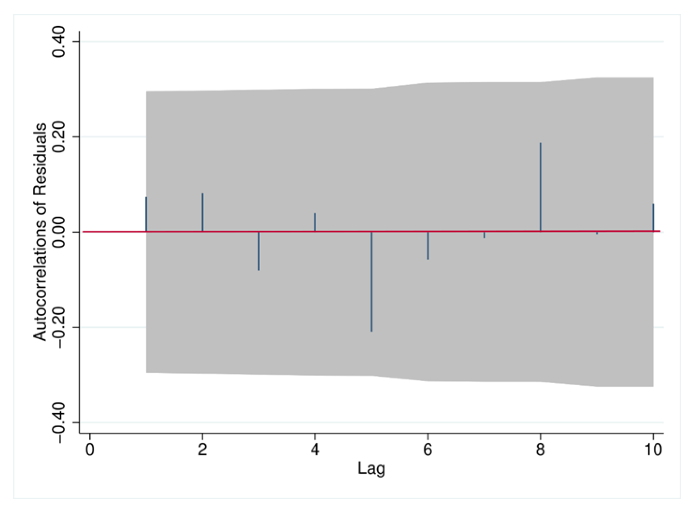
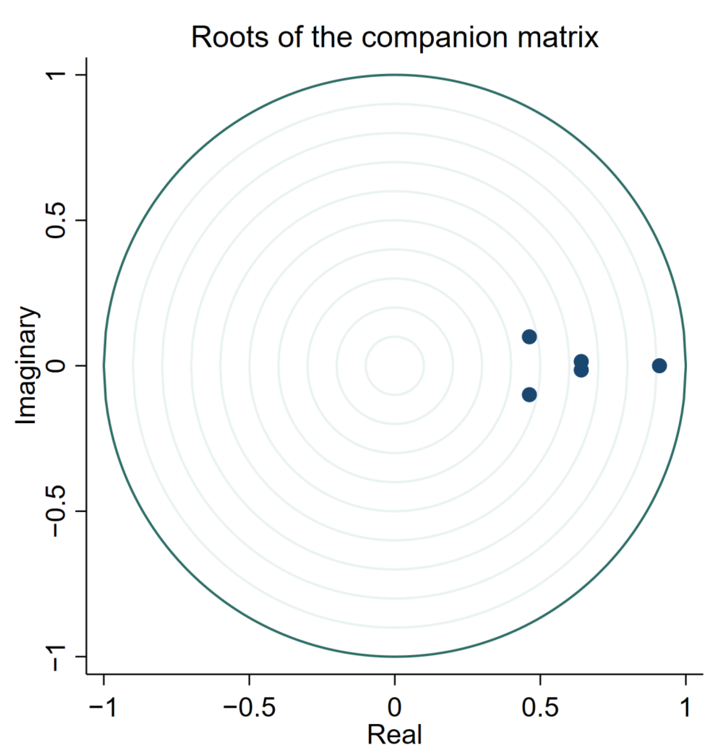
4.1. VARX Model and Data

Given that South Korea is a small open economy, we have constructed a VARX model consisting of two variable blocks. The first block includes foreign variables with significant impacts on the South Korean economy and maritime transport cost variables, which we are interested in; they are entirely exogenous. The second block comprises key variables of the South Korean macroeconomy, which are endogenous. The endogenous variables do not influence the exogenous ones (contemporaneously or with lags). Consequently, we use the following VARX model:
y t = A 0 + A 1 y t 1 + + A p y t p + B 0 x t + u t
where y t and x t represent vectors of endogenous and exogenous variables, respectively. A 0 is a vector of intercepts. A p and B 0 are coefficient matrices. u t is assumed to be white noise, and all leads and lags of x t are unrelated to all leads and lags of the error process u t , that is, x t is assumed to be strictly exogenous [41].
If the VAR system expressed in Equation (84) is stable, we can represent it using the Vector Moving Average (VMA-X) form, as shown in Equation (85),
y t = μ + C L u t + D L x t
where μ represents the time-invariant mean of the process, and u t is the vector of structural shocks. The lag operators C L and D L are matrices of parameters. C L represents the Impulse Response Function (IRF), which illustrates the response of the endogenous variables to a unitary change in a structural shock. The identification of orthogonal shocks is based on the standard Cholesky decomposition. D L corresponds to the dynamic multiplier functions, which reflect the response of endogenous variables to changes in exogenous variables. For a more detailed discussion on the construction and properties of the Impulse Response Function and dynamic multiplier functions, please refer to Lütkepohl [41], Chapters 2 and 10.
The optimal lag order p of the VARX model is determined by using the Akaike Information Criterion (AIC), the Hannan–Quinn Information Criterion (HQIC), and the Schwarz Bayesian Information Criterion (SBIC), the results of which are shown in Table 4. The optimal lag order chosen via the HQIC and SBIC is 1, while the AIC selects the best lag order to be 8. Considering the dense parameterization caused by excessive lag periods, we ultimately choose the lag order p to be 1.
In conjunction with our DSGE theoretical model, we have selected some key variables of the South Korean macroeconomy as the endogenous variables in our model. The vector of endogenous variables is as follows:
y t = G D P   C P I   T O T   E X R A T E   R
where GDP represents real GDP, CPI stands for the consumer price index, TOT refers to the terms of trade, EXRATE signifies the nominal exchange rate, and R is the nominal interest rate. Notably, other crucial candidate variables like the import and export price indices and the producer price index are excluded from the model. This is because, considering Equations (11) and (50), we found that a combination of these three prices, respectively, constitutes the CPI variable and the terms of trade variable. This will lead to severe multicollinearity problems if import and export prices, producer prices, CPI, and terms of trade variables are included in the model simultaneously. Moreover, adding too many variables would exacerbate the dense parameterization of the VARX system. Considering these factors, we opted to use the CPI variable and terms of trade variable in lieu of the import and export price variables and producer price variable for analysis. Lastly, based on the ordering of endogenous variables, we utilize the standard Cholesky decomposition to identify orthogonal shocks. Furthermore, we found that the ordering of endogenous variables does not affect our results. Even if we invert the current ordering and re-estimate the VARX model, the results remain unchanged (these results are omitted for brevity; interested readers can contact the author for details.).
The vector of exogenous variables is as follows:
x t = O I L   R _ U S   C C F I
where the global oil prices (OIL) and the U.S. interest rate (R_US) are representative variables for foreign shocks commonly used in macroeconomic literature (see, Anwar and Nguyen [42], Afrin [43], Pham [44], and Köse and Aslan [45]). CCFI, the China Containerized Freight Index, is used to represent maritime transport costs. The reason for selecting CCFI as a representation of South Korea’s maritime transport costs is detailed in the introduction section of this paper.
This paper employs quarterly data from the first quarter of 2002 to the fourth quarter of 2022 to investigate the impact of changes in maritime transport costs on the South Korean macroeconomy. Definitions and sources of the variables are provided in Table 5. Following Ravn et al. [46], to maintain consistency in the form of variables between the theoretical model and the empirical analysis, we converted all variables into logarithmic form, and used the Hodrick–Prescott (HP) filter (with a smoothing parameter λ of 1600) to remove the trend, i.e., the variable form is the log deviation from the trend.
The presence of unit roots in variables could give rise to spurious regression. As such, we executed a unit root test utilizing the DF-GLS test, currently recognized as one of the most potent unit root tests for single variables [47]. As indicated in Table 6, all variables are found to be stationary.

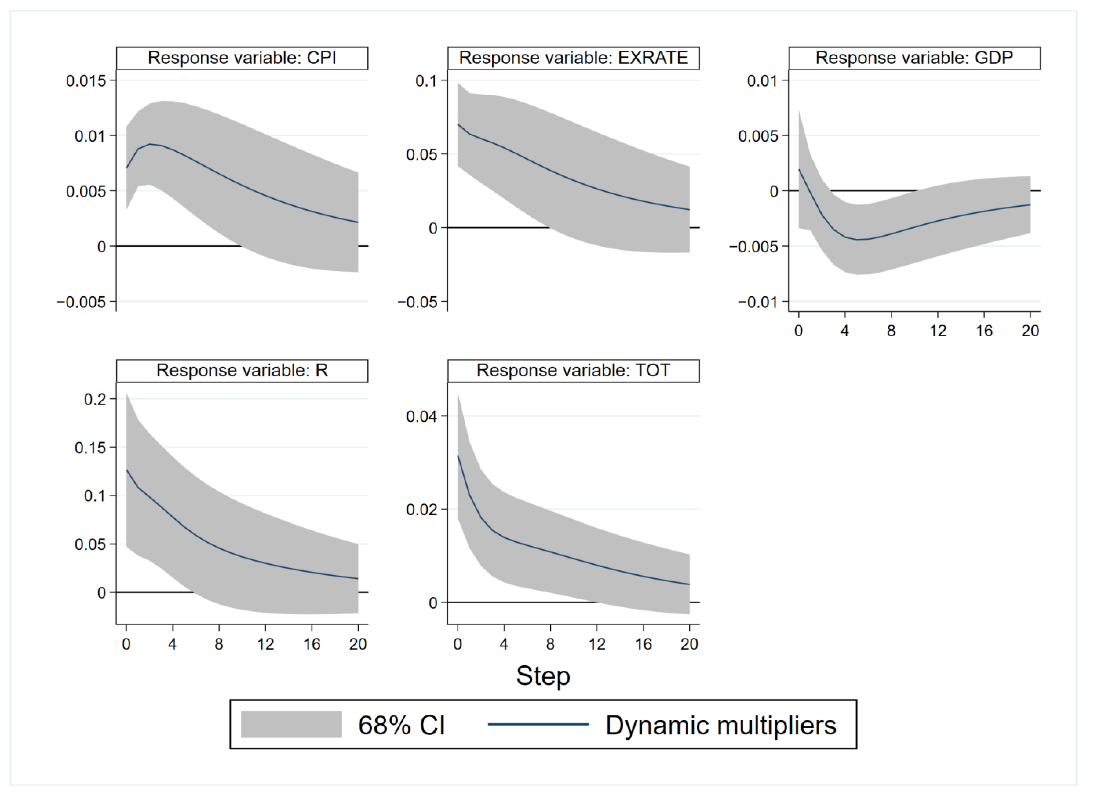
4.2. Analysis of Dynamic Multiplier Functions

Before drawing conclusions from the estimated results, we reviewed the system’s stability within the VARX model. Figure 3 indicates that all inverse roots are within the unit circle, confirming that the estimated VARX is stable.
We determine the impact over time of a one standard deviation increase in the exogenous variables in the VARX system through dynamic multiplier function analysis. Figure 4 depicts the effects of maritime transport cost shocks on domestic variables, accompanied by the corresponding 68% credible sets.
We can observe that an unexpected rise in maritime transport costs leads to an immediate increase in the CPI, which continues to grow for two quarters before gradually declining. The CPI significantly responds to the increase in maritime transport costs over nine quarters. Compared to the theoretical simulation results, the magnitude of the impact on CPI is similar but more persistent. This result is also consistent with the findings of other empirical studies. Carrière-Swallow, Deb, Furceri, Jiménez and Ostry [11] utilized the local projection method to investigate the response of inflation to changes in maritime transport costs, finding that an increase in one standard deviation in maritime shipping costs typically leads to a 0.15 percentage point increase in domestic inflation within 12 months.
The positive shock to maritime transport costs results in a significant increase in terms of trade, which then gradually declines, moving towards its equilibrium value. Both the direction and magnitude of the reaction of the terms of trade are similar to the theoretical simulation results. Upon receiving a shock from maritime transport costs, the nominal interest rate, and nominal exchange rate immediately increase. The direction of their changes is the same as the results of the theoretical simulation, but the magnitude of their increase far exceeds the theoretical simulation results. Although GDP does not immediately respond to the shock in maritime transport costs, GDP decreases gradually in the second quarter and becomes significantly negative in the third quarter. After reaching its lowest point in the fifth quarter, GDP slowly returns to a steady state. The trajectory of GDP change closely resembles the results of the theoretical simulation.
In summary, the outcomes of the empirical analysis fundamentally align closely with those of the theoretical analysis, especially concerning the direction of changes in endogenous variables in the short-term following a shock in maritime transport costs. This corroboration validates the robustness of our theoretical model.

5. Conclusions

This paper is primarily divided into two parts: the theoretical model section and the empirical analysis section. In the theoretical model section, we integrate maritime transport costs into a small open economy DSGE model, characterized by incomplete pass-through in its import and export sectors. Employing parameters consistent with the South Korean economy, we simulate the response of key macroeconomic variables to maritime transport cost shocks. We found that shocks in maritime transport costs lead to deviations from the law of one price in the import and export sectors, driving increases in both export and import prices. The rise in import prices triggers an increase in terms of trade. The escalation in export prices leads to a decrease in export demand, reducing the overall demand for domestic products and causing a decline in domestic product prices. However, the deflationary effect of decreasing domestic product prices cannot compensate for the inflationary impact of the rising import prices, thereby escalating the overall CPI. When foreign prices remain constant, the rise in domestic CPI heightens expectations of currency depreciation. The currency depreciates instantly to adhere to the UIP condition. In line with the Taylor rule, the central bank elevates interest rates to curb inflation. The increase in interest rates curbs total demand, further contracting economic activity and increasing the output gap. In the empirical section, we construct a VARX model incorporating exogenous variable blocks, employing empirical data from South Korea to examine the dynamic relationship between maritime transport cost shocks and macroeconomic variables. The results of the dynamic multiplier functions of the VARX model indicate that the short-term variations in key macroeconomic variables (real output, terms of trade, nominal exchange rate, nominal interest rate, and CPI) following shocks in maritime transport costs align with the impulse response function results simulated by the DSGE model. This validates that our DSGE model can successfully match significant features of South Korean macroeconomic data and capture the importance of maritime transport cost shocks to the South Korean macroeconomy.
In light of the aforementioned main results, we contend that our study, through theoretical models and empirical analysis, reveals the effects of maritime transport costs shocks on key macroeconomic variables such as import and export prices, exchange rates, interest rates, and the CPI. This insight aids governments and businesses in better understanding the impact of maritime transport costs shocks, enabling more targeted responses. Furthermore, our research demonstrates the mechanisms by which maritime transport costs shocks influence exchange rates and inflation, providing beneficial references and theoretical support for central banks in regulating exchange rate policies and formulating inflation control measures. Additionally, governments can adjust trade policies based on the impact of maritime transport costs on import and export prices and trade conditions to balance exports and imports, thereby protecting domestic industries. Our study also presents the consistency between theory and empirical findings by integrating the DSGE and VARX models. This indicates that considering maritime transport costs factors assists in the precise analysis and forecasting of macroeconomic issues, furnishing policymakers with more accurate decision-making bases. Lastly, understanding the influence of maritime transport costs on small open economies (such as South Korea) facilitates coordination and cooperation with major trading partners and international organizations to jointly mitigate adverse shocks and promote global trade and economic stability. Overall, this paper offers significant policy guidance and practical decision-making value for comprehending and addressing the macroeconomic effects brought about by changes in maritime transport costs.
This study has certain limitations. Firstly, our research assumes that maritime transport costs are entirely exogenous to the domestic economy. While this assumption may be reasonable for small open economies, it may not be easy to apply to large economies worldwide. Therefore, in future research, we hope to adjust the model structure to consider the impact of maritime transport costs on large open economies. Secondly, we did not include the government sector in our DSGE model. The government sector can also take measures to deal with shocks in maritime transport costs. For example, following the surge in maritime transport costs due to the COVID-19 outbreak, the South Korean government initiated a freight subsidy plan, ensuring capacity access for small and medium-sized shippers [1]. Therefore, we recommend that future research includes the government sector in the model to provide a basis for examining the effectiveness of related subsidy policies. Furthermore, it would be intriguing to broaden the scope of the current DSGE model to incorporate additional factors alongside applying Bayesian techniques for parameter estimation and replacing the VARX model with a structural VAR model.

Author Contributions

Conceptualization, X.D. and Y.-J.C.; Methodology, X.D.; Software, X.D.; Data curation, X.D.; Writing—original draft, X.D.; Writin—review & editing, Y.-J.C.; Supervision, Y.-J.C.; Funding acquisition, Y.-J.C. All authors have read and agreed to the published version of the manuscript.

Funding

This research received no external funding.

Data Availability Statement

The data presented in this study are available from the authors upon request.

Conflicts of Interest

The authors declare no conflict of interest.

References

  1. United Nations Conference on Trade and Development (UNCTAD). Review of Maritime Transport 2021; UNCTAD: Geneva, Switzerland, 2021. [Google Scholar]
  2. Fernando, L.; Dunn, J. The Dynamics of International Shipping Costs; Federal Reserve Bank of St. Louis: St. Louis, MI, USA, 2022; Available online: https://www.stlouisfed.org/on-the-economy/2022/january/dynamics-international-shipping-costs (accessed on 3 January 2022).
  3. Carrière-Swallow, Y.; Deb, P.; Furceri, D.; Jiménez, D.; Ostry, J.D. How Soaring Shipping Costs Raise Prices around the World; International Monetary Fund: Washington, DC, USA, 2022; Available online: https://www.imf.org/en/Blogs/Articles/2022/03/28/how-soaring-shipping-costs-raise-prices-around-the-world (accessed on 28 March 2022).
  4. Michail, N.A.; Melas, K.D.; Cleanthous, L. The Relationship between Shipping Freight Rates and Inflation in the Euro Area. Int. Econ. 2022, 172, 40–49. [Google Scholar] [CrossRef]
  5. United Nations Conference on Trade and Development (UNCTAD). Container Shipping in Times of COVID-19: Why Freight Rates Have Surged, and Implications for Policymakers; UNCTAD Policy Brief No. 84; UNCTAD: Geneva, Switzerland, 2021. [Google Scholar]
  6. United Nations Conference on Trade and Development (UNCTAD). Shipping During COVID-19: Why Container Freight Rates Have Surged; UNCTAD: Geneva, Switzerland, 2021; Available online: https://unctad.org/news/shipping-during-covid-19-why-container-freight-rates-have-surged (accessed on 23 April 2021).
  7. Rožić, T.; Naletina, D.; Zając, M. Volatile Freight Rates in Maritime Container Industry in Times of Crises. Appl. Sci. 2022, 12, 8452. [Google Scholar] [CrossRef]
  8. Park, J.S.; Seo, Y.-J. The Impact of Seaports on the Regional Economies in South Korea: Panel Evidence from the Augmented Solow Model. Transp. Res. Part E Logist. Transp. Rev. 2016, 85, 107–119. [Google Scholar] [CrossRef]
  9. Ding, X.; Wang, M. Container Freight Rates and International Trade Causality Nexus: Evidence from Panel Var Approach for Shanghai and Asean-6 Countries. Discret. Dyn. Nat. Soc. 2022, 2022, 2415914. [Google Scholar] [CrossRef]
  10. Organisation for Economic Co-operation and Development (OECD). Oecd Economic Outlook; OECD: Paris, France, 2021; Volume 2021. [Google Scholar]
  11. Carrière-Swallow, Y.; Deb, P.; Furceri, D.; Jiménez, D.; Ostry, J.D. Shipping Costs and Inflation. J. Int. Money Financ. 2023, 130, 102771. [Google Scholar] [CrossRef]
  12. Adolfson, M.; Laséen, S.; Lindé, J.; Villani, M. Evaluating an Estimated New Keynesian Small Open Economy Model. J. Econ. Dyn. Control 2008, 32, 2690–2721. [Google Scholar] [CrossRef]
  13. Costa, C.J., Jr. Understanding Dsge Models: Theory and Applications; Vernon Press: Wilmington, DE, USA, 2016. [Google Scholar]
  14. Monacelli, T. Monetary Policy in a Low Pass-through Environment. J. Money Credit. Bank. 2005, 37, 1047–1066. [Google Scholar] [CrossRef]
  15. Nicholson, W.B.; Matteson, D.S.; Bien, J. Varx-L: Structured Regularization for Large Vector Autoregressions with Exogenous Variables. Int. J. Forecast. 2017, 33, 627–651. [Google Scholar] [CrossRef]
  16. OECD/European Union Intellectual Property Office. Misuse of Containerized Maritime Shipping in the Global Trade of Counterfeits; Illicit Trade; OECD Publishing: Paris, France, 2021.
  17. Kim, J.W. What Determines the Volume of Maritime Containers in Korea? KIET Ind. Econ. Rev. 2011, 16, 14–25. [Google Scholar] [CrossRef]
  18. Pham, N.T.A.; Sim, N. Shipping Cost and Development of the Landlocked Developing Countries: Panel Evidence from the Common Correlated Effects Approach. World Econ. 2020, 43, 892–920. [Google Scholar] [CrossRef]
  19. Yin, J.; Shi, J. Seasonality Patterns in the Container Shipping Freight Rate Market. Marit. Policy Manag. 2018, 45, 159–173. [Google Scholar] [CrossRef]
  20. Yonhap, S. Korea Introduces Own Container Cargo Index; Yonhap News Agency: Seoul, Republic of Korea, 2022; Available online: https://en.yna.co.kr/view/AEN20221107007400320 (accessed on 7 November 2022).
  21. Macera, A.P.; Divino, J.A. Import Tariff and Exchange Rate Transmission in a Small Open Economy. Emerg. Mark. Financ. Trade 2015, 51, S61–S79. [Google Scholar] [CrossRef]
  22. Bae, B.-H. Results from the Construction of New Bok-Dsge Model for Economic Forecasting and Policy Analysis. Bank Korea Mon. Bull. 2013, 68, 16–52. [Google Scholar]
  23. Kim, T.B. Analysis on Korean Economy with an Estimated Dsge Model after 2000. KDI J. Econ. Policy 2014, 36, 1–64. [Google Scholar]
  24. Choi, J.; Hur, J. An Examination of Macroeconomic Fluctuations in Korea Exploiting a Markov-Switching Dsge Approach. Econ. Model. 2015, 51, 183–199. [Google Scholar] [CrossRef]
  25. Yie, M.-S.; Yoo, B.H. The Role of Foreign Debt and Financial Frictions in a Small Open Economy Dsge Model. Singap. Econ. Rev. 2016, 61, 1550077. [Google Scholar] [CrossRef]
  26. Kang, H.; Suh, H. Macroeconomic Dynamics in Korea During and after the Global Financial Crisis: A Bayesian Dsge Approach. Int. Rev. Econ. Financ. 2017, 49, 386–421. [Google Scholar] [CrossRef]
  27. Engel, C.; Wang, J. International Trade in Durable Goods: Understanding Volatility, Cyclicality, and Elasticities. J. Int. Econ. 2011, 83, 37–52. [Google Scholar] [CrossRef]
  28. Galí, J.; Monacelli, T. Monetary Policy and Exchange Rate Volatility in a Small Open Economy. Rev. Econ. Stud. 2005, 72, 707–734. [Google Scholar] [CrossRef]
  29. Galí, J. Monetary Policy, Inflation, and the Business Cycle: An Introduction to the New Keynesian Framework and Its Applications; Princeton University Press: Princeton, NJ, USA, 2015. [Google Scholar]
  30. Calvo, G.A. Staggered Prices in a Utility-Maximizing Framework. J. Monet. Econ. 1983, 12, 383–398. [Google Scholar] [CrossRef]
  31. Gao, Y.; Yao, X.; Wang, W.; Liu, X. Dynamic Effect of Environmental Tax on Export Trade Based on Dsge Mode. Energy Environ. 2019, 30, 1275–1290. [Google Scholar] [CrossRef]
  32. Kilian, L.; Zhou, X. Modeling Fluctuations in the Global Demand for Commodities. J. Int. Money Financ. 2018, 88, 54–78. [Google Scholar] [CrossRef]
  33. Kilian, L. Not All Oil Price Shocks Are Alike: Disentangling Demand and Supply Shocks in the Crude Oil Market. Am. Econ. Rev. 2009, 99, 1053–1069. [Google Scholar] [CrossRef]
  34. Borchert, I.; Yotov, Y.V. Distance, Globalization, and International Trade. Econ. Lett. 2017, 153, 32–38. [Google Scholar] [CrossRef]
  35. Luo, M.; Fan, L.; Liu, L. An Econometric Analysis for Container Shipping Market. Marit. Policy Manag. 2009, 36, 507–523. [Google Scholar] [CrossRef]
  36. Das, R.C. Forecasting Incidences of COVID-19 Using Box-Jenkins Method for the Period July 12–Septembert 11, 2020: A Study on Highly Affected Countries. Chaos Solitons Fractals 2020, 140, 110248. [Google Scholar] [CrossRef]
  37. Jiang, Y.; Wei, W.; Das, R.C.; Chatterjee, T. Analysis of the Strategic Emission-Based Energy Policies of Developing and Developed Economies with Twin Prediction Model. Complexity 2020, 2020, 4701678. [Google Scholar] [CrossRef]
  38. Das, R.C. Prediction of Number of Cases and Deaths Due to the Second Wave of COVID-19 Using Arima Model for May 11–June 30, 2021: A Study on India and Its Major States. Asian J. Res. Soc. Sci. Humanit. 2021, 11, 1–27. [Google Scholar] [CrossRef]
  39. Justiniano, A.; Preston, B. Monetary Policy and Uncertainty in an Empirical Small Open-Economy Model. J. Appl. Econom. 2010, 25, 93–128. [Google Scholar] [CrossRef]
  40. Justiniano, A.; Preston, B. Macroeconomic Effects of Energy Price: New Insight from Korea? Mathematics 2022, 25, 93–128. [Google Scholar]
  41. Lütkepohl, H. New Introduction to Multiple Time Series Analysis; Springer Science & Business Media: Berlin, Germany, 2005. [Google Scholar]
  42. Anwar, S.; Nguyen, L.P. Channels of Monetary Policy Transmission in Vietnam. J. Policy Model. 2018, 40, 709–729. [Google Scholar] [CrossRef]
  43. Afrin, S. Monetary Policy Transmission in Bangladesh: Exploring the Lending Channel. J. Asian Econ. 2017, 49, 60–80. [Google Scholar] [CrossRef]
  44. Pham, V.A. Impacts of the Monetary Policy on the Exchange Rate: Case Study of Vietnam. J. Asian Bus. Econ. Stud. 2019, 26, 220–237. [Google Scholar] [CrossRef]
  45. Köse, N.; Aslan, Ç. The Effect of Real Exchange Rate Uncertainty on Turkey’s Foreign Trade: New Evidences from Svar Model. Asia Pac. J. Account. Econ. 2023, 30, 553–567. [Google Scholar] [CrossRef]
  46. Ravn, M.O.; Schmitt-Grohé, S.; Uribe, M. Consumption, Government Spending, and the Real Exchange Rate. J. Monet. Econ. 2012, 59, 215–234. [Google Scholar] [CrossRef]
  47. Baek, J. Not All Oil Shocks on the Trade Balance Are Alike: Empirical Evidence from South Korea. Aust. Econ. Pap. 2022, 61, 291–303. [Google Scholar] [CrossRef]
Figure 1. Autocorrelation of residuals.
Mathematics 11 03668 g001
Figure 2. Impulse response function.
Mathematics 11 03668 g002
Figure 3. Stability condition.
Mathematics 11 03668 g003
Figure 4. Dynamic-multiplier functions.
Mathematics 11 03668 g004
Table 1. Lag-order selection criteria for AR model.
L a g A I C B I C
1 88.9549   * 81.8181   *
2 87.2241 78.3032
3 85.7769 75.0718
4 83.8353 71.3460
5 82.5765 68.3030
6 82.6292 66.5715
Note: * indicates the optimal lag.
Table 2. Structural parameters.
ParameterCalibrationDescriptionSource
Households
β 0.99Discount factorChoi and Hur [24], He and Lee [40]
φ 1.2The inverse of Frisch elasticity of labor supplyBae [22]
σ 0.04Coefficient of risk aversionChoi and Hur [24]
α 0.4Level of economic opennessYie and Yoo [25]
η 4.460Elasticity of substitution between domestic and imported goodsBae [22]
Firms
θ H 0.8Domestic prices stickinessBae [22]
θ F 0.69Import price stickinessBae [22]
θ x 0.82Export price stickinessKang and Suh [26]
Monetary policy rule
τ 1 1.5Inflation reaction coefficient in the Taylor ruleBae [22], Kang and Suh [26], Kim [23]
τ 2 0.2Output gap reaction coefficient in the Taylor ruleBae [22], Kang and Suh [26], Kim [23]
Table 3. Exogenous processes.
ParameterCalibrationDescriptionSource
AR coefficients
ρ a 0.98TechnologyChoi and Hur [24]
ρ m 0.82Maritime transport costsAuthors’ estimate
ρ m y 0.93Impact of foreign output on maritime transportation costsAuthors’ estimate
ρ y 0.49Foreign OutputChoi and Hur [24]
ρ i 0.85Foreign interest ratesChoi and Hur [24]
ρ π 0.76Foreign InflationChoi and Hur [24]
ρ i 0.9Interest rate smoothingBae [22], Kang and Suh [26], Kim [23]
Standard deviations
σ a 2 3.06TechnologyChoi and Hur [24]
σ m 2 0.08Maritime transport costsAuthors’ estimate
σ y 2 0.41Foreign OutputChoi and Hur [24]
σ π 2 0.41Foreign interest ratesChoi and Hur [24]
σ i 2 0.52Foreign InflationChoi and Hur [24]
σ z 2 0.002Monetary policy exogenous shocksBae [22]
Table 4. Lag order selection criteria for VARX model.
L a g A I C H Q I C S B I C
0 22.8629 22.6178 22.2495
1 26.8516 26.3001   * 25.4715   *
2 26.8103 25.9524 24.6636
3 26.8465 25.6821 23.9331
4 26.8814 25.4107 23.2013
5 28.0712 26.294 23.6244
6 28.1646 26.0811 22.9511
7 28.0166 25.6266 22.0364
8 28.4341   * 25.7377 21.6872
Note: * indicates the optimal lag.
Table 5. Definition of variables and data sources.
Variable DefinitionAbbreviationPeriodSource
Domestic block (Endogenous variables)
Seasonally Adjusted Real GDPGDP2002:Q1–2022:Q4Bank of Korea’s Economic Statistics System database (BOK-ECOS)
Nominal exchange rate (base rate of KRW to USD)EXRATE2002:Q1–2022:Q4BOK-ECOS
Nominal interest rate (unsecured overnight borrowing rate)R2002:Q1–2022:Q4BOK-ECOS
Terms of TradeTOT2002:Q1–2022:Q4BOK-ECOS
Seasonally Adjusted Consumer Price IndexCPI2002:Q1–2022:Q4BOK-ECOS
Foreign block (Exogenous variables)
West Texas Intermediate (WTI) crude oil priceOIL2002:Q1–2022:Q4Energy Information Administration
U.S. Federal Funds RateR_US2002:Q1–2022:Q4Board of Governors of the Federal Reserve System
China Containerized Freight IndexCCFI2002:Q1–2022:Q4Shanghai Shipping Exchange
Table 6. Unit root tests.
V a r i a b l e D F G L S S t a t i s t i c
G D P 4.285  
T O T 3.668  
C P I 4.038  
E X R A T E 3.639  
R 4.761  
C C F I 3.617  
R _ U S 4.322  
O I L 4.235  
Notes: 1. *** (**) indicates rejection of the original hypothesis with unit root at 1% (5%) significance. 2. The optimal lag order for the DF-GLS test is chosen according to the Schwert Information Criterion (SIC).
Disclaimer/Publisher’s Note: The statements, opinions and data contained in all publications are solely those of the individual author(s) and contributor(s) and not of MDPI and/or the editor(s). MDPI and/or the editor(s) disclaim responsibility for any injury to people or property resulting from any ideas, methods, instructions or products referred to in the content.

