Graph Convolutional Network Design for Node Classification Accuracy Improvement

Abstract

Graph convolutional networks (GCNs) provide an advantage in node classification tasks for graph-related data structures. In this paper, we propose a GCN model for enhancing the performance of node classification tasks. We design a GCN layer by updating the aggregation function using an updated value of the weight coefficient. The adjacency matrix of the input graph and the identity matrix are used to calculate the aggregation function. To validate the proposed model, we performed extensive experimental studies with seven publicly available datasets. The proposed GCN layer achieves comparable results with the state-of-the-art methods. With one single layer, the proposed approach can achieve superior results.

1. Introduction

Graph data structures represent complex data structures for solving different problem domains. Graphs are irregular in shape and can represent any form of relationship between different entities. The ubiquitous representation of graphs is an attractive feature for data processing. Machine learning models are proven to be very efficient in learning different relationships between inputs and outputs and are widely adopted in various research areas [1]. In most cases, deep learning algorithms are capable of capturing hidden patterns in Euclidean data that are not represented in graph form [2]. In recent years, the study of graph neural networks (GNNs) has been growing at a rapid pace. The use of GNNs is mainly focused on graph-oriented data which are very complicated in nature. In a graph, the relationship is built upon nodes and edges, where each node or edge is assigned with features or attributes. These features are revalued vectors that represent original or synthetic data. By using these feature vectors, GNNs can learn the different patterns of relationships or labels associated with each node. Graph learning can be applied to various problems like community detection [3,4], node classification [5,6], link prediction [7], molecular properties, natural language processing, and clustering [8,9].

Among the different applications of GNNs, node classification has gained researchers’ attention. Various approaches are made to the training and prediction capability of GNNs using deep learning approaches. The authors in [10] proposed a node-feature-based learning embedding function which generalizes to unseen nodes. In [11], the graph convolution is formulated as an integral transform of the embedding function under probability measures to identify sample loss and gradients. The study presented in [12] introduced NodeNet, a method for classifying nodes in citation graphs. Prakash et al. [13] proposed the kernel propagation method, leveraging higher-order structural features of GNNs. Additionally, in [14], the authors proposed a two-layer feature selection graph neural network to learn the importance of features during the training period.

A graph convolutional network (GCN) was proposed in [5] for first-order approximations of spectral graph convolutions. The GCN provided significant processing power on graph data and has already been implemented in various tasks [15]. The main categories of the research area where the GCN was implemented include science, computer vision, and natural language processing [16]. The GCN has also been used in drug development and discovery by considering molecular properties and activity prediction [17]. By combining one-hop local graph topologies with node characteristics, graph convolutional networks apply a spectral strategy to learn node embeddings and extract embeddings from the hidden layers. The authors of [18] proposed a model which uses multiple instances of GCNs over node pairs discovered at different distances in random walks, and combined instances are used to learn classification outputs. The study in [19] predicted the interface between pairs of proteins using graph representation of the underlying protein structure. Graph convolution is used by a merge layer and a fully connected layer to make the classification of proteins. A geometric GCN was proposed in [20] to transductive learning on graphs. The authors of [21] proposed improved identification of influential nodes using information entropy and the weighted degree of edge connections. The method was evaluated by comparing nine algorithms and nine datasets. Geometric aggregation including node embedding, structural neighborhood and bi-level aggregation was applied to a graph neural network to obtain good performance. A Lanczos network was proposed in [22], which leverages the Lanczos algorithm to build low rank approximations of the graph Laplacian for graph convolution. A GCN was proposed in [23] for hyperspectral image classification using the minibatch technique, which allows large-scale data to be trained efficiently. In another study in [24], a cluster GCN was proposed to reduce the computational cost for high dataset sizes. In addition, a GCN cannot properly distinguish graph structures and it also suffers from noise limitation. If the data noise increases, the possibility of obtaining good results decreases. From the above discussion, we can observe that different works have been proposed for enhancing graph data classification. Most of the studies concentrate on performing experiments outside of the GCN layer internal structure by introducing new algorithms, minibatch sizes, or changing application areas. However, more research is needed to find a more accurate layer design in order to find an alternative solution for the graph data structure. The motivation of our study is to examine the result when we modify the layer calculation strategy of the following GCN-based approach. In our study, we propose a GCN model for the node classification task. In this study, we have considered the node classification problem for one single graph. We have formed a new GCN layer for enhancing the feature extraction process and classification accuracy. We take the feature propagation mechanism to aggregate the neighborhood information of a particular node. We first normalize the input feature values and next we calculate the coefficient value for aggregation. The coefficient values for each step are updated during the training process. We conduct experiments using the following seven datasets to evaluate the proposed GCN model: Cora, Citeseer, PubMed, Amazon photos, Amazon computers, Cora Full, and Coauthor CS. The experimental results demonstrate promising outcomes achieved by our proposed model. In summary, the main contributions of this study are:

• We propose a GCN layer for improving the classification accuracy of nodes in graph data.
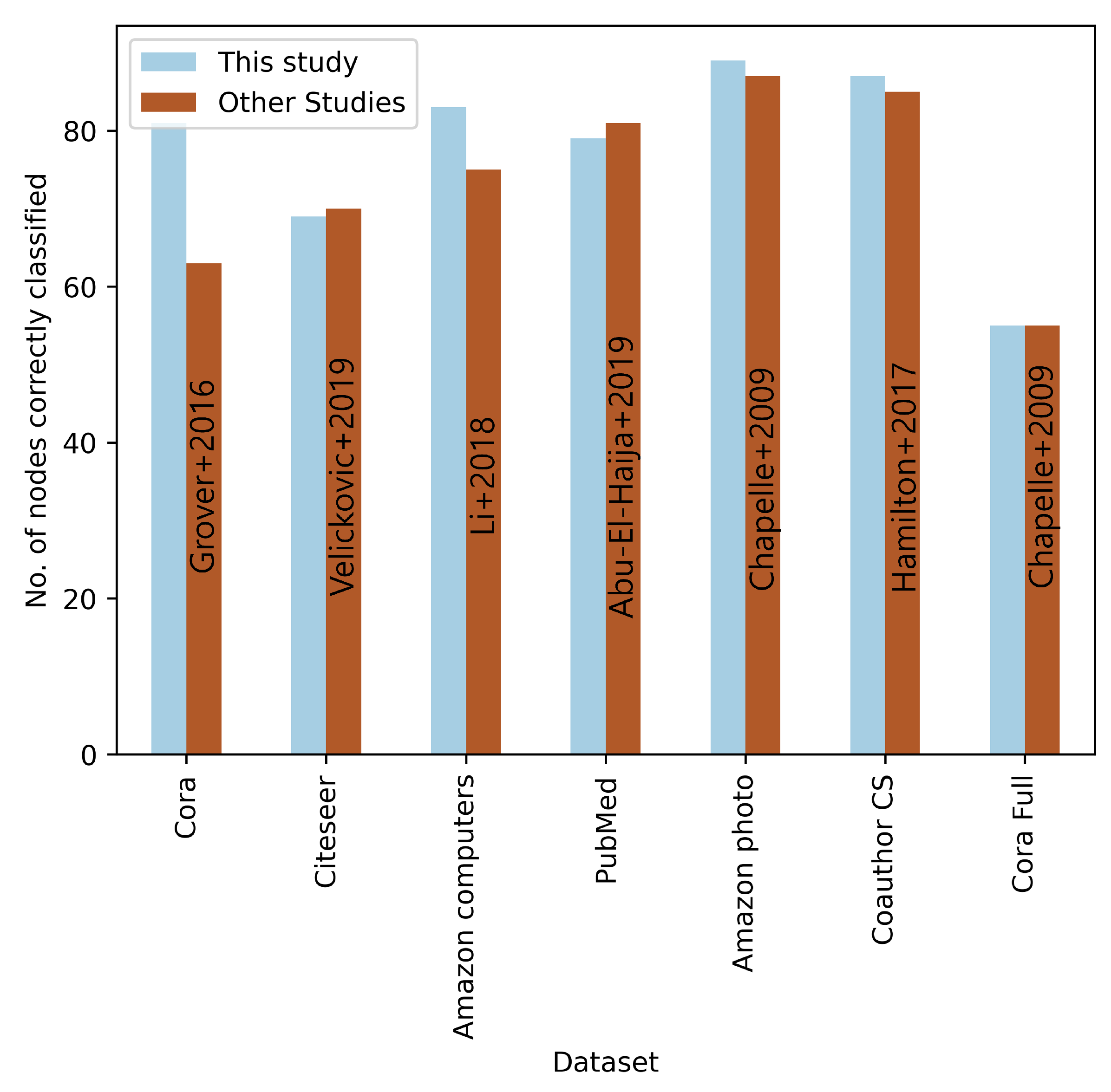
• The proposed approach is tested with seven different datasets and is compared with related previous studies.

The rest of the paper is organized as follows. Section 2 presents the graph notation and GCN structure details, Section 3 demonstrates the proposed model, Section 4 presents the experiment results, and Section 5 concludes the paper.

2. Graph Architecture

2.1. Graph Notation

A graph can be represented as $\mathcal{G}=(\mathcal{V},\mathcal{E})$, where $\mathcal{V}$ is the set of vertices or nodes and $\mathcal{E}$ is the set of edges. We consider that the node sets are $\mathcal{V}=n_1,n_2,....,n_n$ and the edges sets are $\mathcal{E}=e_1,e_2,....,e_m$. An example of a graph structure is represented in Figure 1. This example figure represents 50 nodes with a total number of edges of 252. To process graph data, any graph is represented as an adjacency matrix denoted by $\mathbf{A}\in {\{0,1\}}^{n\times n}$. For each element or node, if there exists an edge between node $v_i$ and $v_j$, ${\mathbf{A}}_{i,j}=1$; if there is no edge, ${\mathbf{A}}_{i,j}=0$. Again, each node is associated with a d-dimension feature matrix $\mathbf{X}\in {\mathbb{R}}^{n\times d}=[{\mathbf{x}}_{\mathbf{1}},{\mathbf{x}}_{\mathbf{2}},...,{\mathbf{x}}_{\mathbf{n}}]$, where ${\mathbf{x}}_{\mathbf{i}}$ is the signal vector for the i-th node. If self-loops are available in the graph structure, the adjacency matrix can be written as $\widehat{\mathbf{A}}=\mathbf{A}+\mathbf{I}$, where $\mathbf{I}$ is the identity matrix. A list of notation is presented in

Table 1. List of notation.

Parameter	Symbol
Graph	$\mathcal{G}$
Set of node or vertices	$\mathcal{V}$
Set of edges	$\mathcal{E}$
Adjacency matrix	$\mathbf{A}$
Feature matrix	$\mathbf{X}$
Signal vector	$\mathbf{x}$
GNN output at the lth layer	$q_n^{\left(l\right)}$
Weight matrix	$\mathbf{W}$
Identity matrix	$\mathbf{I}$
Activation matrix	$\mathbf{H}$
Activation function	$\sigma$
Sigmoid function	$S\left(\right)$
Output of final layer	Y
Model depth	K

.

2.2. Graph Convolutional Networks

GCNs are created by following the neural network architecture using convolution layers to learn node embedding by aggregation. In particular, GCNs use the graph structure and input features to learn the node embedding. A node’s representation captures the structural information within its l-hop network neighborhood after finishing l iterations of aggregation. Mathematically, the l-th layer of a GNN can be represented as follows [25]:

$$q_n^{\left(l\right)}=AGGREGAT{E}^{\left(l\right)}\left(\right\{{\mathbf{x}}_u^{(l-1)}:u\in \mathcal{N}\left(n\right)\left\}\right)$$

(1)

where ${\mathbf{x}}_u^{(l-1)}$ is the feature vector of node u at the l-th layer. A multi-layer GCN can be expressed as follows [5]:

$${\mathbf{H}}^{(l+1)}=\sigma \left({\widehat{\mathbf{C}}}^{-\frac{1}{2}}\widehat{\mathbf{A}}{\widehat{\mathbf{C}}}^{-\frac{1}{2}}{\mathbf{H}}^{\left(l\right)}{\mathbf{W}}^{\left(l\right)}\right),$$

(2)

where $\widehat{\mathbf{A}}$ is the adjacency matrix represented by $\widehat{\mathbf{A}}=\mathbf{A}+\mathbf{I}$, C and W are layered specific trainable weight matrices, $\sigma (.)$ is the activation function, and ${\mathbf{H}}^{(l+1)}$ is the matrix of activations in the $(l+1)$-th layer. If the graph $\mathcal{G}$ can be divided into subgraphs, the convolution layers can be approximated by Monte Carlo sampling. Equation (2) can be expressed as follows [16]:

$${\mathbf{H}}^{l+1}(v,:)=\sigma \left(\frac{1}{f_l}\sum _{i=1}^{f_l}\widehat{\mathbf{A}}(v,u_i^{\left(l\right)})\mathbf{H}(u_i^{\left(l\right)},:){\mathbf{W}}^{\left(l\right)}\right),$$

(3)

where $f_l$ is the number of independent and identically distributed samples $u_1^l,...,u_{f_l}^l$ for Monte Carlo samplings. A GCN can be built by stacking multiple convolution layers and a simple example of a single layer is as follows:

$$\mathbf{H}=f(\mathbf{X},\mathbf{A})=\widehat{\mathbf{A}}ReLU\left(\widehat{\mathbf{A}}\mathbf{X}\mathbf{W}\right),$$

(4)

where $f(\mathbf{X},\mathbf{A})$ is the learning condition of a model, where $\mathbf{X}$ is the data feature and $\mathbf{A}$ is the adjacency matrix, and $ReLU$ is the rectified linear unit non-linearity. The expression in (4) is useful to understand the formation of GCN layers and the architecture of a GCN model.

3. Proposed Model

In this section, we describe the proposed GCN model in detail. The architecture of the proposed model is shown in Figure 2. First, we have the input layer which accepts the graph parameters and includes an adjacency matrix and input features. The feature values are normalized in the first place, which can be expressed as follows:

$$\widehat{\mathbf{X}}=\frac{\mathbf{X}}{{\mathbf{X}}_0},$$

(5)

where ${\mathbf{X}}_0$ is the maximum value. Next, the normalized features are passed through a GCN layer which is shown in Figure 2. In the GCN layer, several operations are performed in a sequential manner. In the first step, the input weights are normalized using the softmax function as follows:

$${\mathbf{W}}_{i+1}=\sigma \left({\mathbf{W}}_i\right),$$

(6)

where ${\mathbf{W}}_{i+1}$ are the update weights and ${\mathbf{W}}_i$ are the received weights. In the next step, we create a coefficient for aggregation using the following expression:

$$\mathcal{A}={\mathbf{W}}_{(\mathbf{i}+\mathbf{1})\left[\mathbf{0}\right]}\times \mathbf{I}+{\mathbf{W}}_{(\mathbf{i}+\mathbf{1})\left[\mathbf{1}\right]}\times (\mathbf{I}+\mathbf{A}),$$

(7)

where the first value of the update weight is multiplied by the identity matrix and the second weight value is multiplied by the adjacent matrix and identity matrix. The resulting value is multiplied by the feature matrix. The expression of aggregation is written as follows:

$$\mathbf{H}=\mathcal{A}\times \overline{\mathbf{X}}\times {\mathbf{W}}_{(\mathbf{i}+\mathbf{1})}+b,$$

(8)

where b is the bias value. The resulting value is passed through by the sigmoid layer as follows:

$$\widehat{\mathbf{H}}=S\left(\mathbf{H}\right),$$

(9)

where $S(.)$ is the sigmoid function. The loss is estimated using cross entropy loss. The overall process of the GCN layer is shown in Algorithm 1. After the GCN layer, a softmax function is applied for predicting one of the classes. Finally, the result with the highest probability is picked as the predicted class. The proposed single layer network can be expressed as follows:

$$Y=f(X,A)=\sigma \left(S\left(\mathbf{A}\widehat{\mathbf{X}}{\mathbf{W}}_{i+1}\right)\right).$$

(10)

Algorithm 1 Graph Convolution Layer

Input $\mathbf{X}$, $\mathbf{W},\mathbf{I},\mathbf{A}$     Output: l, $\mathcal{G}$ 1: $\overline{\mathbf{X}}=\mathbf{X}/{\mathbf{X}}_{\mathbf{0}}$ 2: ${\mathbf{W}}_{\mathbf{i}+\mathbf{1}}=\sigma \left({\mathbf{W}}_{\mathbf{i}}\right)$ 3: $\mathcal{A}={\mathbf{W}}_{(\mathbf{i}+\mathbf{1})\left[\mathbf{0}\right]}\ast \mathbf{I}+{\mathbf{W}}_{(\mathbf{i}+\mathbf{1})\left[\mathbf{1}\right]}\ast (\mathbf{I}+\mathbf{A})$ 4: $\mathbf{H}=\mathcal{A}\ast \overline{\mathbf{X}}\ast {\mathbf{W}}_{(\mathbf{i}+\mathbf{1})}+b$ 5: $\overline{\mathbf{H}}=S\left(\mathbf{H}\right)$ 6: $l,\mathcal{G}=L_{CE}\left(\overline{\mathbf{H}}\right)$ 7: End.

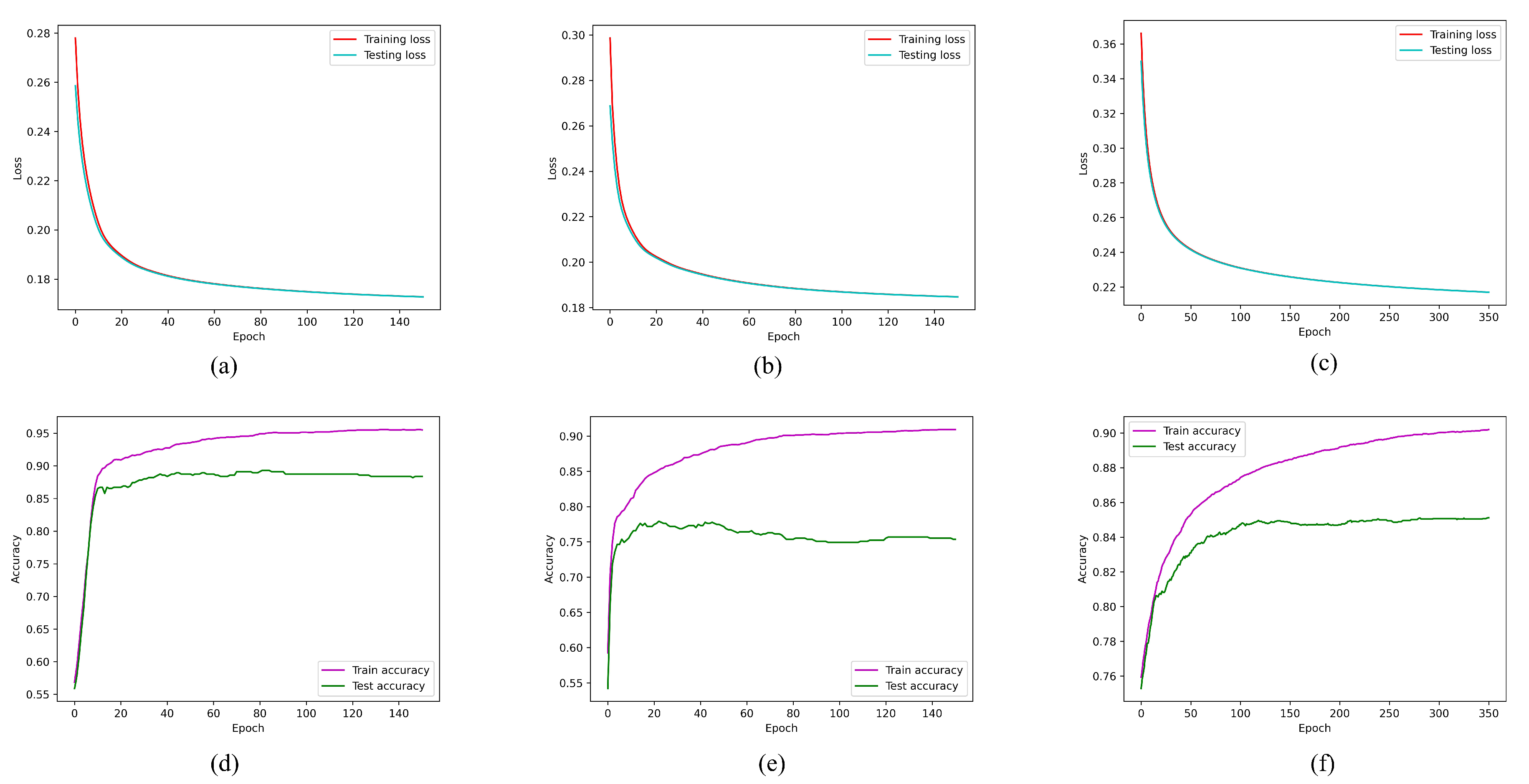
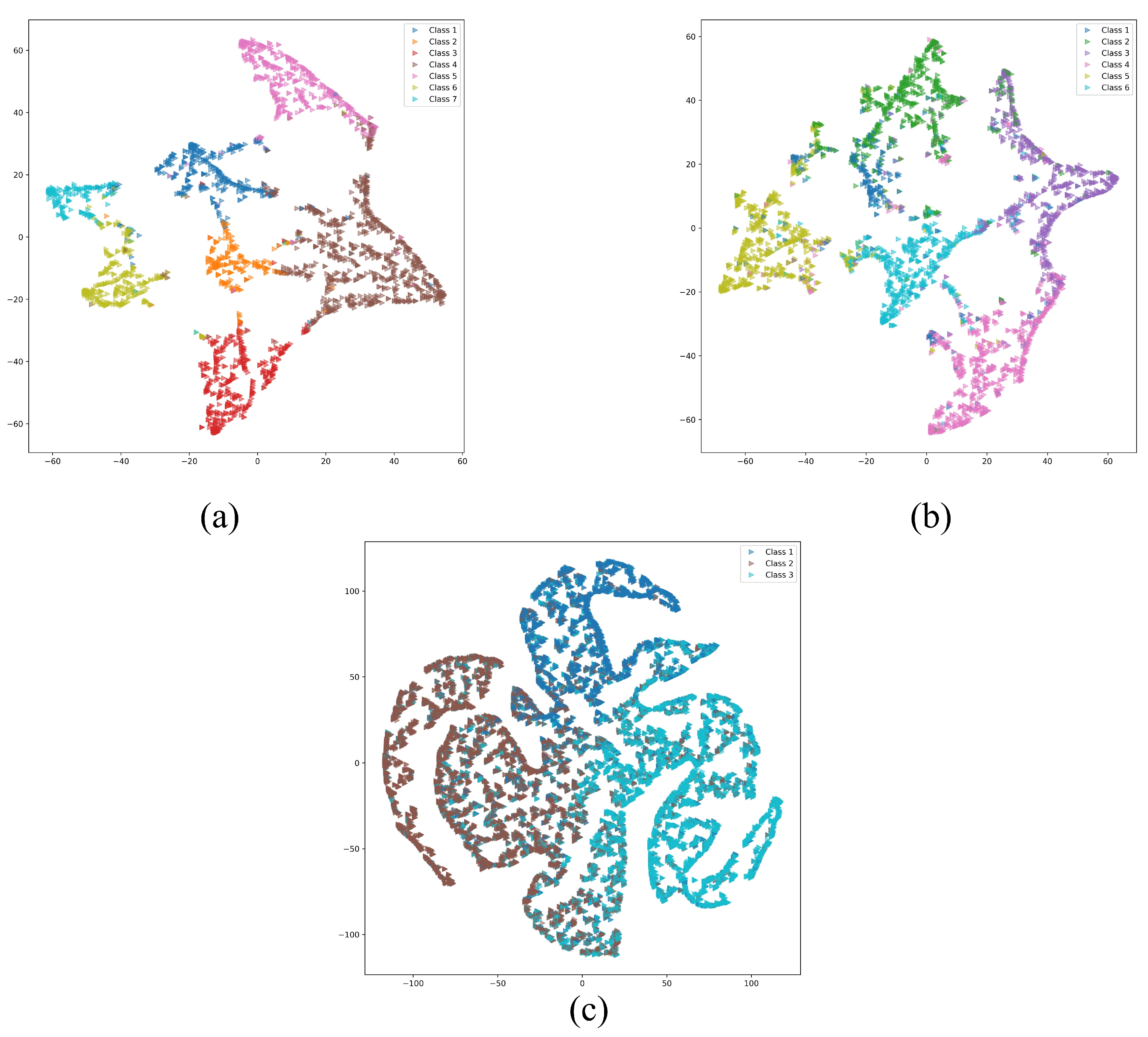
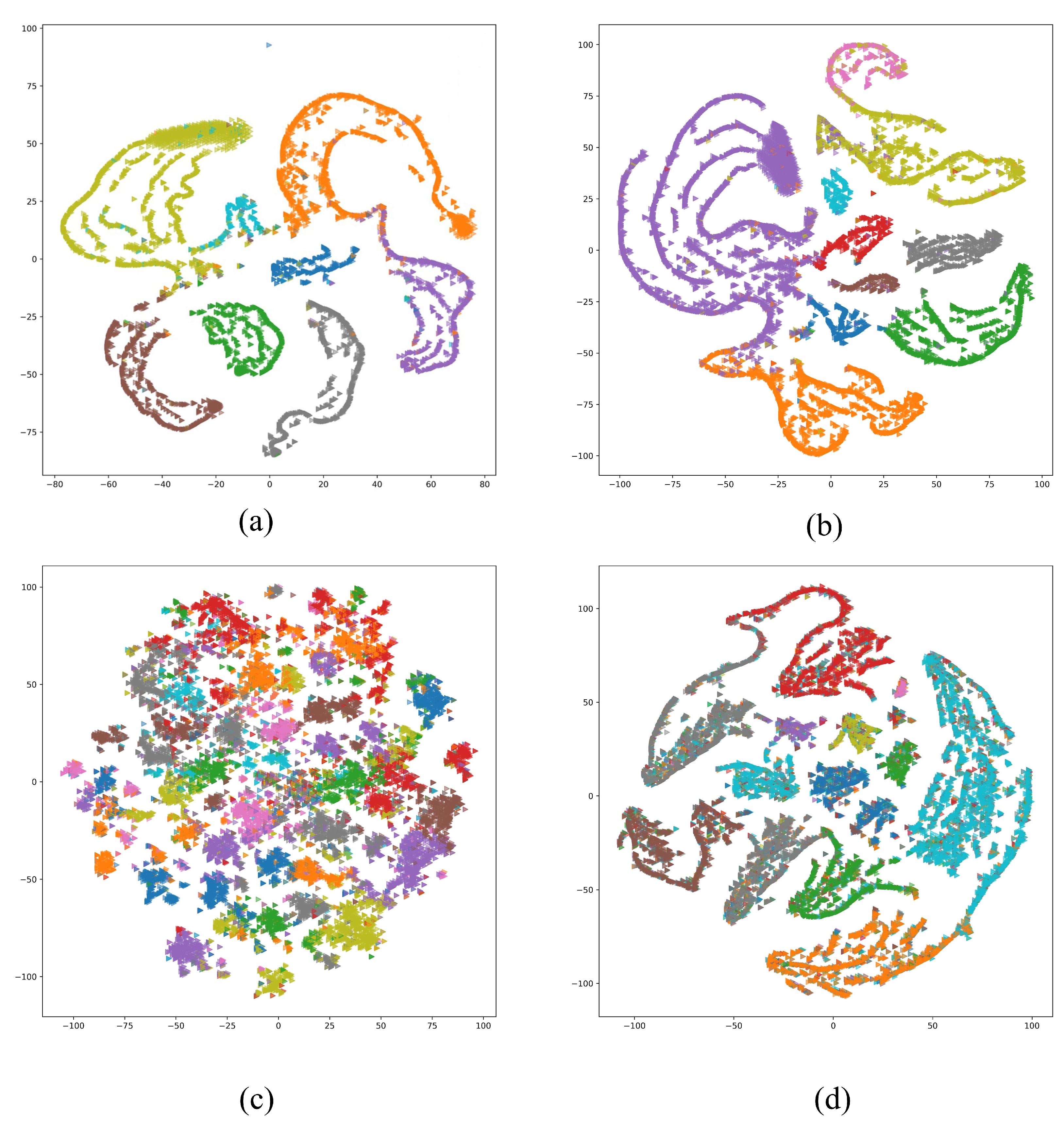
4. Results

In any machine-learning-based problem solving approach, the objective is to minimize the loss for the objective function and gain a high accuracy. In our approach, we also try to minimize the loss, which will eventually result in a high node classification accuracy. The overall learning and inference process for node classification of the proposed algorithm is described in Algorithm 2. In the first place, we set learning parameters, which are updated in order to minimize the loss function.

Algorithm 2 Proposed model training and evaluation steps.

1: Input: Train data feature ($\mathbf{X}$), labels(y), Adjacency matrix ($\mathbf{A})$, Loss function, optimizer(Adam), coefficient value (q), max-episode. 2: Output: Optimized model. 3: A learnable parameters list is created with size of $prarameters=\left(\right(\mathbf{X},y),q)$. 4: Adam optimizer function is initiated. for episode is not max-episode do    5: Get parameters state.    6: Using Algorithm 1 calculate the loss for the current parameters.    7: Update the value of parameters using the optimizer function. end for 8: Save the model with the minimized loss value. 9: Return the model. 10: Run inference for the input feature and find node class. 11: End

Algorithm 1 is the main function to reduce the loss for the input graph data. We use the adjacency matrix and identity matrix to reduce the loss. After some episodes, the loss starts to be minimized because the internal calculation can correctly match the label associated with the data.

To evaluate the performance of the proposed GCN model, we have considered seven publicly available datasets, namely Cora, Citeseer, PubMed, Amazon photos, Amazon computers, Cora Full, and Coauthor CS. Each dataset’s information is listed in

Table 2. Experiment dataset information.

Dataset	Nodes	Edges	Features	Labels	Label Rate	Edge Density
Cora [26]	2708	5429	1433	7	0.0563	0.0004
Citeseer [27]	3327	4732	3703	6	0.0569	0.0004
Pubmed [28]	19,717	44,338	500	3	0.0030	0.0001
Amazon photo [29]	7487	119,043	745	8	0.0214	0.0011
Amazon computers [29]	13,752	491,722	767	10	0.0149	0.0007
Cora Full [30]	19,793	65,311	8710	70	0.0745	0.0001
Coauthor CS [29]	18,333	163,788	6805	15	0.0149	0.0007

. The Cora dataset has 2708 nodes of a citation network of machine learning papers and seven different classes that represent different subject categories [26]. The Citeseer dataset has 3327 nodes and six classes that represent subject categories. Similarly, PubMed has 19,717 nodes with three classes. We also considered large datasets which include more nodes and classes, such as Amazon photos, Amazon computer, Cora Full, and Coauthor CS. These datasets are large compared to the dataset which is described above, and all the information in the datasets is provided in Table 2. First, we considered the Cora dataset for evaluating our proposed model. Figure 3a shows the overall training and testing loss of the model for the Cora dataset. We observed a sharp decrease in loss after 20 episodes and later, the loss reduces steadily. Again, Figure 3d shows the accuracy of the model for the training and testing process. The mean value of the testing accuracy is around $87.25\%$. Next, the Citeseer dataset was considered for model evaluation. In Figure 3b, we can see the training and testing loss for the Citeseer dataset. The loss trend is similar to the previously described Cora dataset. However, the accuracy is a bit different in the case of the Citeseer dataset, as depicted in Figure 3e. The training accuracy increases steadily but the testing accuracy fluctuates and sometimes decreases. Nevertheless, the mean accuracy for testing remains at $76\%$ which is comparable with existing results in the literature. The training and testing progress for the PubMed dataset is shown in Figure 3c, and Figure 3f shows the achieved accuracy during training. As the model learns and updates the optimized parameters, better accuracy results are produced. The training accuracy increases to $84.18\%$ as the number of epochs increases. However, the test accuracy does not increase in the same manner, and this is due to the randomness of the dataset. Figure 4 shows the training and testing loss and accuracy for the four other datasets. Figure 4a shows the training and testing loss, which is reduced to the minimum after 150 epochs. The accuracy also reaches high values at around 150 epochs, as depicted in Figure 4e. The mean test accuracy for the Amazon photo dataset is $89.60\%$ which is comparable to other studies. Again, Figure 4b shows the training and testing of loss for dataset of Amazon computers. The testing accuracy is different to the training accuracy, but both follow the same trend, as depicted in Figure 4f, and the method can achieve the highest accuracy of $81.88\%$. The Cora Full dataset has the highest number of classes, and achieving a good testing accuracy is challenging. Figure 4c,g shows the loss and accuracy for training and testing data. Finally, the Coauthor CS dataset was considered and achieves a $92.42\%$ testing accuracy. The loss and accuracy are shown in Figure 4d,h, respectively. In

Table 3. A comparison of model testing accuracy with state-of-the-art methods for the Cora, Citeseer, and PubMed datasets.

Ref.	Method	Classification Data	Cora	Citeseer	Pubmed
[9]	Node2vec	$\mathbf{A}$	$68.66\pm 1.83$%	$47.98\pm 1.75$%	$72.36\pm 0.95$%
[31]	GAT	$\mathbf{A},\mathbf{I},\mathbf{Y}$	$82.40\pm 0.62$%	$71.25\pm 0.43$%	$83.90\pm 0.70$%
[31]	GAT	$\mathbf{A},\mathbf{X},\mathbf{Y}$	$83.34\pm 0.47$%	$72.71\pm 0.52$%	$83.90\pm 0.70$%
[32]	JK NET	$\mathbf{A},\mathbf{I},\mathbf{Y}$	$82.40\pm 0.62$%	$71.25\pm 0.43$%	$84.50\pm 0.80$%
[33]	APPNP	$\mathbf{A},\mathbf{X},\mathbf{Y}$	$85.79\pm 0.27$%	$75.97\pm 0.46$%	$83.37\pm 0.32$%
[34]	APPNP	$\mathbf{A},\mathbf{I},\mathbf{Y}$	$84.70\pm 0.30$%	$71.25\pm 0.27$%	$84.10\pm 0.72$%
[35]	ConfGNN	$\mathbf{A},\mathbf{X},\mathbf{I},\mathbf{Y}$	$82.0\pm 0.30$%	$72.7\pm 0.8$%	$79.40\pm 0.30$%
[18]	NGCN	$\mathbf{A},\mathbf{X},\mathbf{Y}$	$82.3\pm 0.6$%	$71.4\pm 1.0$%	$80.20\pm 0.70$%
[36]	GIL	$\mathbf{A},\mathbf{X},\mathbf{Y}$	$82.0\pm 1.1$%	$71.2\pm 1.0$	$78.0\pm 0.70$%
[37]	AGSN	$\mathbf{A},\mathbf{X},\mathbf{Y}$	$83.8\pm 0.3$	$74.5\pm 0.4$%	$79.90\pm 0.30$%
This study	GCN	$\mathbf{A},\mathbf{X},\mathbf{I},\mathbf{Y}$	$\mathbf{87}.\mathbf{25}\pm \mathbf{0}.\mathbf{051}\%$	$\mathbf{76}.\mathbf{00}\pm \mathbf{0}.\mathbf{21}$%	$\mathbf{84}.\mathbf{18}\pm \mathbf{0}.\mathbf{0168}$%

Boldface characters in column classification data are matrix and boldface in column Cora, Citeseer and Pubmed represents highest accuracy.

, we have compared the result obtained in our experiment with other studies. It can be observed that the proposed model can achieve better performance compared to other studies. However, for PubMed it has a marginal advantage. The other four dataset results have been benchmarked in

Table 4. A comparison of model testing accuracy with state-of-the-art methods for the Amazon photos, Amazon computers, Cora Full, and Coauthor CS datasets.

Ref.	Method	Classification Data	Amazon Photo	Amazon Computers	Cora Full	Coauthor CS
[38]	LabelProp NL	$\mathbf{X},\mathbf{W},\mathbf{Y}$	$81.02\pm 2.89$%	$74.24\pm 3.94$%	$45.99\pm 1.53$%	$72.89\pm 2.52$%
[10]	GraphSAGE	$\mathbf{X},\mathbf{W}$, K, $\mathbf{Y}$	$79.90\pm 2.30$%	$75.68\pm 3.32$%	$58.05\pm 0.67$%	$87.05\pm 0.90$%
[39]	DGI	$\mathbf{X},\mathbf{A}$	$86.34\pm 1.87$%	$77.40\pm 2.15$%	$59.37\pm 0.67$%	$89.42\pm 0.78$%
[40]	Co-training	$\mathbf{X},\mathbf{A},\mathbf{W},\mathbf{Y}$	$71.85\pm 5.09$%	$77.26\pm 3.85$%	$55.37\pm 1.17$%	$91.60\pm 0.32$%
[5]	GCN	$\mathbf{X},\mathbf{A},\mathbf{W},\mathbf{Y}$	$88.84\pm 2.85$%	$81.46\pm 2.78$%	$60.99\pm 0.60$%	$90.92\pm 0.46$%
[41]	GAT	$\mathbf{X},\mathbf{W},\mathbf{Y}$	$88.32\pm 2.05$%	$76.51\pm 2.25$%	$61.28\pm 0.44$%	$89.65\pm 0.37$%
[42]	MCL-GCNs	$\mathbf{X},\mathbf{A}$	$\mathbf{91}.\mathbf{54}\pm \mathbf{0}.\mathbf{59}\%$	$81.86\pm 2.77$%	$\mathbf{61}.\mathbf{47}\pm \mathbf{0}.\mathbf{49}\%$	$90.57\pm 0.68$%
This study	GCN	$\mathbf{A},\mathbf{X},\mathbf{I},\mathbf{Y}$	$89.60\pm 0.13$%	$\mathbf{81}.\mathbf{88}\pm \mathbf{0}.\mathbf{13}\%$	$59.47\pm 0.88$%	$\mathbf{92}.\mathbf{42}\pm \mathbf{0}.\mathbf{22}\%$

Boldface characters in column classification data are matrix and boldface in column Amazon Photo, Amazon Computers, Cora Full, and Coauthor CS represents highest accuracy.

. The proposed model significantly achieves good results in the case of the Coauthor CS dataset. In the case of other datasets, the results are comparable with most studies, except that some studies can provide better results.

Node embedding results can be helpful to understand the evaluation performance of any model. The node embedding will converge to the same class of labels and form a cluster. Figure 5a shows node embedding classification for the Cora dataset. We can observe from Figure 5a that seven different clusters have been formed after training. Each of the clusters represents a specific topic of the Cora dataset. Figure 5b shows node embedding of the classes in the Citeseer dataset. It was observed that six different clusters have formed after training. For the PubMed dataset, three different classes are shown in Figure 5c. There are some overlaps with the different classes because some nodes are not correctly classified. For the other four datasets, the node embedding results are presented in Figure 6. For clear visibility, we have omitted the legends for the dataset classes. Figure 6a–d shows the node embedding results for the Amazon photos, Amazon computers, Cora Full, and Coauthor CS datasets, respectively. After training, the algorithm can successfully cluster similar nodes, which signifies the node classification accuracy. In summarizing the model’s performance based on the experimental results, it is evident that the proposed GCN layer with a single layer can achieve superior results on the Cora, Citeseer, and PubMed datasets. For the Amazon photos, Amazon computers, and Cora Full datasets, the model does not surpass the performance of existing models. However, it consistently produces results that are nearly identical to those of the compared studies. Notably, the proposed model demonstrates outstanding performance on the Coauthor CS dataset.

We also conducted a node classification accuracy test with the highest probability for each of the datasets. We selected 100 data samples randomly and tested the trained model. The classification results are presented in Figure 7, which compares the outcomes with various existing studies. For the Cora dataset, out of 100 test data points, our model correctly classifies 80% of nodes. In contrast, the method described in [9] achieves an accuracy of 63%. When the Citeseer dataset is considered, the percentage of accurately classified nodes drops to 70%, while the approach outlined in [31] also achieves a 70% accuracy. The PubMed dataset demonstrates a node classification accuracy of 79%, whereas the study conducted in [18] achieves a slightly higher accuracy of 81%. Moving to the Amazon computers dataset, our model achieves a commendable 83% accuracy, comparable to [40], which attained a 75% accuracy. Similarly, the Amazon photos dataset achieves an accuracy of 89%, slightly surpassing the performance in [38] at 87%. In the context of the Coauthor CS dataset, our model achieves an 88% accuracy, which can be contrasted with [10], boasting an accuracy of 85%. However, the Cora Full dataset exhibits the lowest accuracy at approximately 55%, aligning with similar findings in [38], who also reported an accuracy of 55%. It is important to note that these results can vary due to the random nature of the experiments and their sensitivity to different parameter settings.

The complexity of the proposed model depends on the following equation:

$$\mathbf{H}={\mathbf{W}}_{(\mathbf{i}+\mathbf{1})\left[\mathbf{0}\right]}\ast \mathbf{I}+{\mathbf{W}}_{(\mathbf{i}+\mathbf{1})\left[\mathbf{1}\right]}\ast (\mathbf{I}+\mathbf{A})\ast \overline{\mathbf{X}}\ast {\mathbf{W}}_{(\mathbf{i}+\mathbf{1})}.$$

(11)

To express the complexity, we consider the number of nodes to be N and the number of embedding dimensions to be F. Thus, we can express each $\mathbf{W}$ as ($F\times F$), $\mathbf{A}$ as ($N\times N$), and $\mathbf{X}$ as ($N\times F$). By following the above Equation (11), we can express the complexity as $\mathcal{O}(2N^{3}F+N{F}^3)$.

5. Conclusions

In this paper, we have proposed a GCN layer for enhancing the accuracy of GCN-based node classification operations. We have proposed a new GCN layer combined with the use of weight, adjacency, and identity matrices to improve prediction. The experimental results show that our proposed model can achieve more than $87\%$ accuracy for the Cora dataset, 76% for the Citeseer dataset, and 84% for the PubMed dataset. For the other four datasets (Amazon photos, Amazon computer, Cora Full, and Coauthor CS), 89%, 81%, 59%, and 92% accuracies were achieved, respectively. As the number of classes increases, the proposed model cannot correctly classify all nodes. In our future studies, we will work on datasets that include more classes.

References

- Zhang, W.; Chien, J.; Yong, J.; Kuang, R. Network-based machine learning and graph theory algorithms for precision oncology. NPJ Precis. Oncol. 2017, 1, 25. [Google Scholar] [CrossRef] [PubMed]
- Wu, Z.; Pan, S.; Chen, F.; Long, G.; Zhang, C.; Philip, S.Y. A comprehensive survey on graph neural networks. IEEE Trans. Neural Netw. Learn. Syst. 2020, 32, 4–24. [Google Scholar] [CrossRef] [PubMed]
- Girvan, M.; Newman, M.E. Community structure in social and biological networks. Proc. Natl. Acad. Sci. USA 2002, 99, 7821–7826. [Google Scholar] [CrossRef] [PubMed]
- Rosvall, M.; Bergstrom, C.T. Maps of random walks on complex networks reveal community structure. Proc. Natl. Acad. Sci. USA 2008, 105, 1118–1123. [Google Scholar] [CrossRef] [PubMed]
- Kipf, T.N.; Welling, M. Semi-supervised classification with graph convolutional networks. arXiv 2016, arXiv:1609.02907. [Google Scholar]
- Li, B.; Pi, D. Learning deep neural networks for node classification. Expert Syst. Appl. 2019, 137, 324–334. [Google Scholar] [CrossRef]
- Ying, R.; He, R.; Chen, K.; Eksombatchai, P.; Hamilton, W.L.; Leskovec, J. Graph convolutional neural networks for web-scale recommender systems. In Proceedings of the 24th ACM SIGKDD International Conference on Knowledge Discovery & Data Mining, London, UK, 19–23 August 2018; pp. 974–983. [Google Scholar]
- Perozzi, B.; Al-Rfou, R.; Skiena, S. Deepwalk: Online learning of social representations. In Proceedings of the 20th ACM SIGKDD International Conference on Knowledge Discovery and Data Mining, New York, NY, USA, 24–27 August 2014; pp. 701–710. [Google Scholar]
- Grover, A.; Leskovec, J. node2vec: Scalable feature learning for networks. In Proceedings of the 22nd ACM SIGKDD International Conference on Knowledge Discovery and Data Mining, San Francisco, CA, USA, 13–17 August 2016; pp. 855–864. [Google Scholar]
- Hamilton, W.; Ying, Z.; Leskovec, J. Inductive representation learning on large graphs. Adv. Neural Inf. Process. Syst. 2017, 30, 1025–1035. [Google Scholar]
- Chen, J.; Ma, T.; Xiao, C. Fastgcn: Fast learning with graph convolutional networks via importance sampling. arXiv 2018, arXiv:1801.10247. [Google Scholar]
- Dabhi, S.; Parmar, M. Nodenet: A graph regularised neural network for node classification. arXiv 2020, arXiv:2006.09022. [Google Scholar]
- Prakash, S.K.A.; Tucker, C.S. Node classification using kernel propagation in graph neural networks. Expert Syst. Appl. 2021, 174, 114655. [Google Scholar] [CrossRef]
- Maurya, S.K.; Liu, X.; Murata, T. Simplifying approach to node classification in Graph Neural Networks. J. Comput. Sci. 2022, 62, 101695. [Google Scholar] [CrossRef]
- Wang, T.; Jin, D.; Wang, R.; He, D.; Huang, Y. Powerful graph convolutional networks with adaptive propagation mechanism for homophily and heterophily. In Proceedings of the AAAI Conference on Artificial Intelligence, Virtual conference, 22 Feburary–1 March 2022; Volume 36, pp. 4210–4218. [Google Scholar]
- Zhang, S.; Tong, H.; Xu, J.; Maciejewski, R. Graph convolutional networks: A comprehensive review. Comput. Soc. Netw. 2019, 6, 1–23. [Google Scholar] [CrossRef]
- Sun, M.; Zhao, S.; Gilvary, C.; Elemento, O.; Zhou, J.; Wang, F. Graph convolutional networks for computational drug development and discovery. Briefings Bioinform. 2020, 21, 919–935. [Google Scholar] [CrossRef] [PubMed]
- Abu-El-Haija, S.; Kapoor, A.; Perozzi, B.; Lee, J. N-gcn: Multi-scale graph convolution for semi-supervised node classification. In Proceedings of the 35th Uncertainty in Artificial Intelligence Conference, Tel Aviv, Israel, 22–25 July 2019; pp. 841–851. [Google Scholar]
- Fout, A.; Byrd, J.; Shariat, B.; Ben-Hur, A. Protein interface prediction using graph convolutional networks. Adv. Neural Inf. Process. Syst. 2017, 30, 6533–6542. [Google Scholar]
- Pei, H.; Wei, B.; Chang, K.C.C.; Lei, Y.; Yang, B. Geom-gcn: Geometric graph convolutional networks. arXiv 2020, arXiv:2002.05287. [Google Scholar]
- Dong, S.; Zhou, W. Improved influential nodes identification in complex networks. J. Intell. Fuzzy Syst. 2021, 41, 6263–6271. [Google Scholar] [CrossRef]
- Liao, R.; Zhao, Z.; Urtasun, R.; Zemel, R.S. Lanczosnet: Multi-scale deep graph convolutional networks. arXiv 2019, arXiv:1901.01484. [Google Scholar]
- Hong, D.; Gao, L.; Yao, J.; Zhang, B.; Plaza, A.; Chanussot, J. Graph convolutional networks for hyperspectral image classification. IEEE Trans. Geosci. Remote Sens. 2020, 59, 5966–5978. [Google Scholar] [CrossRef]
- Chiang, W.L.; Liu, X.; Si, S.; Li, Y.; Bengio, S.; Hsieh, C.J. Cluster-gcn: An efficient algorithm for training deep and large graph convolutional networks. In Proceedings of the 25th ACM SIGKDD International Conference on Knowledge Discovery & Data Mining, Anchorage, AK, USA, 4–8 August 2019; pp. 257–266. [Google Scholar]
- Xu, K.; Hu, W.; Leskovec, J.; Jegelka, S. How powerful are graph neural networks? arXiv 2018, arXiv:1810.00826. [Google Scholar]
- Sen, P.; Namata, G.; Bilgic, M.; Getoor, L.; Galligher, B.; Eliassi-Rad, T. Collective classification in network data. AI Mag. 2008, 29, 93. [Google Scholar] [CrossRef]
- Rossi, R.; Ahmed, N. The network data repository with interactive graph analytics and visualization. In Proceedings of the AAAI Conference on Artificial Intelligence, Austin, TX, USA, 25–30 January 2015; Volume 29. [Google Scholar]
- Namata, G.; London, B.; Getoor, L.; Huang, B.; Edu, U. Query-driven active surveying for collective classification. In Proceedings of the 10th International Workshop on Mining and Learning with Graphs, Edinburgh, Scotland, 1 July 2012; Volume 8, p. 1. [Google Scholar]
- McAuley, J.; Targett, C.; Shi, Q.; Van Den Hengel, A. Image-based recommendations on styles and substitutes. In Proceedings of the 38th International ACM SIGIR Conference on Research and Development in Information Retrieval, Santiago, Chile, 9–13 August 2015; pp. 43–52. [Google Scholar]
- Bojchevski, A.; Günnemann, S. Deep gaussian embedding of graphs: Unsupervised inductive learning via ranking. arXiv 2017, arXiv:1707.03815. [Google Scholar]
- Velickovic, P.; Fedus, W.; Hamilton, W.L.; Liò, P.; Bengio, Y.; Hjelm, R.D. Deep graph infomax. ICLR (Poster) 2019, 2, 4. [Google Scholar]
- Xu, K.; Li, C.; Tian, Y.; Sonobe, T.; Kawarabayashi, K.I.; Jegelka, S. Representation learning on graphs with jumping knowledge networks. In Proceedings of the International Conference on Machine Learning, Stockholm, Sweden, 10–15 July 2018; pp. 5453–5462. [Google Scholar]
- Gasteiger, J.; Bojchevski, A.; Günnemann, S. Predict then propagate: Graph neural networks meet personalized pagerank. arXiv 2018, arXiv:1810.05997. [Google Scholar]
- Gasteiger, J.; Weißenberger, S.; Günnemann, S. Diffusion improves graph learning. Adv. Neural Inf. Process. Syst. 2019, 32, 1336–13378. [Google Scholar]
- Vashishth, S.; Yadav, P.; Bhandari, M.; Talukdar, P. Confidence-based graph convolutional networks for semi-supervised learning. In Proceedings of the 22nd International Conference on Artificial Intelligence and Statistics, Naha, Okinawa, Japan, 16–18 April 2019; pp. 1792–1801. [Google Scholar]
- Zhu, S.; Pan, S.; Zhou, C.; Wu, J.; Cao, Y.; Wang, B. Graph geometry interaction learning. Adv. Neural Inf. Process. Syst. 2020, 33, 7548–7558. [Google Scholar]
- Zheng, R.; Chen, W.; Feng, G. Semi-supervised node classification via adaptive graph smoothing networks. Pattern Recognit. 2022, 124, 108492. [Google Scholar] [CrossRef]
- Chapelle, O.; Scholkopf, B.; Zien, A. Semi-supervised learning (chapelle, o. et al., eds.; 2006)[book reviews]. IEEE Trans. Neural Netw. 2009, 20, 542. [Google Scholar] [CrossRef]
- Veličković, P.; Fedus, W.; Hamilton, W.L.; Liò, P.; Bengio, Y.; Hjelm, R.D. Deep graph infomax. arXiv 2018, arXiv:1809.10341. [Google Scholar]
- Li, Q.; Han, Z.; Wu, X.M. Deeper insights into graph convolutional networks for semi-supervised learning. In Proceedings of the AAAI Conference on Artificial Intelligence, Orleans, LA, USA, 2–7 February 2018; Volume 32. [Google Scholar]
- Velickovic, P.; Cucurull, G.; Casanova, A.; Romero, A.; Lio, P.; Bengio, Y. Graph attention networks. Stat 2017, 1050, 10–48550. [Google Scholar]
- Xu, H.; Jiang, B.; Huang, L.; Tang, J.; Zhang, S. Multi-head collaborative learning for graph neural networks. Neurocomputing 2022, 499, 47–53. [Google Scholar] [CrossRef]