Abstract
The concept of the hybrid structure, as an extension of both soft sets and fuzzy sets, has gained significant attention in various mathematical and decision-making domains. In this paper, we delve into the realm of hemirings and investigate the properties of hybrid h-bi-ideals, including prime, strongly prime, semiprime, irreducible, and strongly irreducible ones. By employing these hybrid h-bi-ideals, we provide insightful characterizations of h-hemiregular and h-intra-hemiregular hemirings, offering a deeper understanding of their algebraic structures. Beyond theoretical implications, we demonstrate the practical value of hybrid structures and decision-making theory in handling real-world problems under imprecise environments. Using the proposed decision-making algorithm based on hybrid structures, we have successfully addressed a significant real-world problem, showcasing the efficacy of this approach in providing robust solutions.
Keywords:
prime; strongly prime; semiprime; irreducible and strongly irreducible hybrid h-bi-ideals; decision making MSC:
94D05
1. Introduction
L. A. Zadeh in 1965 [1] initiated the concept of fuzzy sets, the best framework for addressing uncertainties and imprecise information. Fuzzy set is defined by its membership function, whose values are defined on the closed interval [0, 1]. This approach extends the generalized theory of uncertainty described in [2] to a broader context. Numerous works [3,4,5] are based on the idea of fuzzy set theory, its extensions, and applications.
Modelling uncertain data is a challenge for researchers in a variety of disciplines, including economics, engineering, environmental science, sociology, and medical science. Classical methods might not always be adequate to deal with uncertainties appearing in these domains. Although mathematical methods like rough sets [6], fuzzy sets [1], and other mathematical tools [7] are frequently employed to express uncertainty, Molodtsov [8] highlighted that each has its own challenges. Molodtsov offered a novel method to model ambiguity and uncertainty as a result [8]. Many researchers contributed to extending soft sets with fuzzy set theory [9,10,11]. Fuzzy soft sets are an extension introduced by Maji et al. [12] and provide a more flexible approach to handling uncertainty. Since then there has been a rapid growth of interest in soft sets and their various applications to algebraic systems [13,14,15,16,17,18,19,20], data analysis [21], and decision making under uncertainty [22,23,24,25,26].
Hemirings are thought of as a generalization of rings and refer to an additively commutative semiring with zero members. Ideals of hemirings play a significant part in the theories of algebraic structure. K-ideals are a special type of ideal, studied by Henriksen [27], while h-ideals are a more restrictive class of ideals, proposed by Iizuka [28]. H-ideals and k-ideals have been implemented in hemirings by [29]. The generalization of the theory of h-ideals is called fuzzy h-ideals of hemirings [30]. By utilizing the fuzzy h-ideals, Zhan et al. [31] explored the h-hemiregular hemirings. Furthermore, the concepts of fuzzy h-bi-ideals and fuzzy h-quasi-ideals of hemirings are extended in [32]. A prime h-bi-ideal [33] is an extension of h-bi-ideals that has an additional property (defined in Section 2). The concept of fuzzy prime h-bi-ideals [33] refers to a fuzzified variant of prime h-bi-ideals, where degrees of membership are used to define how much an element belongs to the fuzzy prime h-bi-ideal rather than strict inclusion.
Jun et al. [34] developed the idea of a hybrid structure as a parallel circuit of fuzzy sets and soft sets by integrating the notions of soft sets and fuzzy sets. In hybrid structures, fuzzy sets are utilized to represent negative membership, while set-valued mappings are employed to represent positive membership. Algebric structures, for example, BCK/BCI algebras and semigroups are studied in relation to the concept of the hybrid structure [35,36,37,38,39]. To deal with uncertainty and imprecision, hybrid structures are implemented in hemirings by incorporating the concepts of soft sets and fuzzy sets. In order to apply the hemiring framework, it is necessary to define operations that take into account both fuzzy and soft sets [40,41]. This enables a more thorough approach to knowledge representation, problem-solving, and decision-making in uncertain situations. Asmat et al. [41] assessed the hybrid structure in hemirings and investigated several properties of hybrid h-ideals, hybrid h-bi-ideals, and hybrid h-quasi-ideals. The characterizations of h-hemiregular hemirings are discussed and several important results of a h-hemiregular hemirings are provided. This paper proposes prime hybrid h-bi-ideals which is an extension of hybrid h-bi-ideals [41] and we aim to investigate various aspects of hemirings. Also, this work has conducted a characterization of certain classes of hemirings based on these prime hybrid h-bi-ideals. Furthermore, we illustrate the importance of the defined hybrid structure in the decision-making process with the help of examples from real-world situations to explore new directions in algebraic development and tackle practical problems with improved uncertainty-handling abilities by utilising hybrid structures in hemirings.
The arrangement of paper is given as follows. The basic concepts and preliminary results concerning hemirings and hybrid structures, which will be used throughout this paper, are provided in Section 2. Section 3 provides the concepts of prime (semiprime, strongly prime) hybrid h-bi-ideals and the characterization of some classes of hemings in terms of these hybrid h-bi-ideals has been carried out. In the final part of the paper, we present a hybrid structure-based decision-making algorithm and use it to solve a problem that exists in the real world.
2. Preliminaries
We give a concise overview of the fundamental ideas and concepts employed in hemirings.
A nonempty set with “∔” and “⋄” as binary operations on is said to be a semiring if and are semigroups and the following laws
A member 0 of a semiring is said to be zero if and only if all of its members satisfy the conditions and . Hemirings are semirings ( that contain zero members and are commutative with regard to addition “∔”.
The sum and product of and where and are provided in a hemiring by
When a subset of a hemiring is closed under addition and multiplication while , the subset is said to be a bi-ideal.
Let the set for some is referred to as h-closure of .
For a bi-ideal of a hemiring if , and implies then is said to be an h-bi-ideal (H-BI) of
An ideal in satisfying is referred to as an h-idempotent ideal of a hemiring .
Proposition 1
([33]). If and are the H-BI of a hemiring , following that is an H-BI of .
Definition 1
([33]). If implies or ) for all H-BI and of following that H-BI of a hemiring is known as a prime (semiprime) H-BI of
Definition 2
([33]). If indicating or for all H-BI and of a hemiring then the H-BI of is said to be strongly prime.
A hemiring is h-hemiregular (H-HemiR) if there exists satisfying for any
If there exist and such that , then a hemiring is said to be h-intra-hemiregular (H-IHemiR) for each .
By a fuzzy subset of a non-empty set , we mean a mapping
, from a non-empty set within unit interval.
If and are fuzzy subsets of then the fuzzy subsets are defined as:
and for all
The term “soft set” over is a mapping of £ into the set of all subsets of i.e., , where is the initial universe set, ¥ is a collection of attributes that the entities in hold, and is the power set of .
Basic Operations of Hybrid Structures
Definition 3
([34]). A hybrid structure (ḦyS) in a set of parameters over an initial universe set is defined as:
Definition 4.
Let us represent the set of all ḦyS in over by Here, we define an order in :
The hybrid intersection of two hybrid structures and in over is defined as:
Definition 5.
The hybrid union of two hybrid structures and in over is defined as:
The hybrid framework described by
Definition 6
([41]). Let and be two ḦyS in over The hybrid h-sum ⊞ is defined as:
Each , , , , , ∈ , where, the symbols for supremum and infimum are ⊎ and respectively.
Definition 7.
which is concisely represented by ⊠ , where, the definitions of and are given as:
and
where, , , , , , ∈
Let and be two ḦyS in a hemiring over The hybrid h-product ⊠ is defined as
Definition 8
([41]). A hybrid h-bi-ideal (ḦyH-BI) in upon is defined to be a if ∀ , we have
- (1)
- (2)
- (3)
- (4)
- (5)
- (6)
- (7)
- (8)
3. Prime Hybrid H-bi-Ideals
In this section, the concept of prime, strongly prime, semiprime, irreducible and strongly irreducible ḦyH-BI are provided with examples. The characterization of H-HemiR and H-IHemiR hemirings by these ḦyH-BI is also discussed.
Definition 9.
A ḦyH-BI of over is called a prime hybrid h-bi-ideal (PḦyH-BI) if suggests or for every ḦyH-BI and of upon
Example: Suppose that there are five houses in the initial universe set given by = {}. Let a set of parameters = {,,,} be a set of status of houses in which stands for the parameter “beautiful”, stands for the parameter “cheap”, stands for the parameter “in good location”, stands for the parameter “in green surrounding”. We define the binary operation ⋄ and ∔ on by the Cayley table in Table 1.

Table 1.
Cayley table for the binary operations ∔ and ⋄.
Then (,∔,⋄) is a hemiring. Let and be a any ḦyH-BI in over which is given by Table 2, Table 3 and Table 4.
Table 2.
Tabular representation of ḦyH-BI
Table 3.
Tabular representation of ḦyH-BI
Table 4.
Tabular representation of ḦyH-BI
It is routine calculation to verify that if and implies or and or for all ,,, in This implies that gives or . Thus is a prime ḦyH-BI of over
Definition 10.
A ḦyH-BI of over is said to be strongly prime hybrid h-bi-ideal (StPḦyH-BI) if for all ḦyH-BI and of over ( implies or (see the related example in Appendix A i.e., Example A1).
Definition 11.
A ḦyH-BI of over is idempotent if .
Definition 12.
A semiprime hybrid h-bi-ideal (briefly SPḦyH-BI) is defined to be a ḦyH-BI in over satisfying means for every single ḦyH-BI of upon (see the related example in Appendix A i.e., Example A2).
Further, we demonstrate that the hybrid h-product of any two ḦyH-BI of over is similar to ḦyH-BI in the following proposition.
Proposition 2.
is an ḦyH-BI of over whereas, and be any ḦyH-BI of over
Proof.
Let and be any ḦyH-BI of over and Then
and
whereas, At this point
and
To prove that , implies and Similarly, is obtained by combining and This results in the equation and Due to this,
and
Now
and
Also,
and
Consequently, is likewise a ḦyH-BI of over □
The intersection of any collection of ḦyH-BI of over is shown to be a ḦyH-BI in the ensuing Lemma 1.
Lemma 1.
For a collection of ḦyH-BI of over their intersection is also a ḦyH-BI of over
Proof.
is a collection of ḦyH-BI of over We have to prove that is a ḦyH-BI of over Let then
and
and
and
and
□
The result given below tells us that the intersection of a family of prime hybrid h-bi-ideals in a hemring over is semiprime.
Lemma 2.
If is a member of the family of PḦyH-BI of over and subsequently is a SPḦyH-BI of over
Proof.
Assume that is an element of a collection of PḦyH-BI of over Lemma 1 states that is a ḦyH-BI of over . Consequently, we acquire that for all if ( for any ḦyH-BI of . Since each is a PḦyH-BI of over eventually for all . Therefore □
Definition 13.
An irreducible (strongly irreducible) hybrid h-bi-ideal Ir(SIr)ḦyH-BI of over is an ḦyH-BI in such a manner that implies or or whereas , are ḦyH-BI of over
We demonstrate that every strongly irreducible semiprime ḦyH-BI of upon is a StPḦyH-BI in the paragraph that follows.
Theorem 1.
Every strongly irreducible, SPḦyH-BI of over is a StPḦyH-BI.
Proof.
Assume that be a strongly irreducible, SPḦyH-BI of over Let and are ḦyH-BI of over such that ( Since and so ( and ( Thus ( This implies that because is a SPḦyH-BI of Since is SIrḦyH-BI of over or . □
4. Hemirings in Which Each Hybrid H-bi-Ideal Is Strongly Prime
The hemirings in which each ḦyH-BI is semiprime are studied in this part of the paper. Furthermore, we talk about the hemirings in which each ḦyH-BI is strongly prime.
Proposition 3.
Let and and be a ḦyH-BI of over defined by Then ∃ an IrḦyH-BI of upon with and defined by
Proof.
Let is a ḦyH-BI of defined by with . Now let is a collection of ḦyH-BI of and the elements of this collection are partially ordered. Let and is totally ordered. Then is a ḦyH-BI of such that Clearly, when we take we get
and
and
and
and
Thus is a ḦyH-BI of over Since for all we have Also ( Thus and is an upper bound of . The existence of a maximalḦyH-BI of is declared by Zorn’s Lemma and is defined by also Let for any ḦyH-BI of We get and It is obvious that or We claim that and Then Thus, (, and a contradiction arises to our supposition that Hence, or Therefore, is an IrḦyH-BI of over
The following theorem investigates the H-HemiR and H-IHemiR hemirings for which each ḦyH-BI is semiprime. □
Theorem 2.
The following statements have similar results in :
- (1)
- is H-HemiR and H-IHemiR hemiring at the same time.
- (2)
- For each single ḦyH-BI of over .
- (3)
- With and selected at random ḦyH-BI of over ,
- (4)
- Every ḦyH-BI of over results in an SPḦyH-BI.
- (5)
- Every proper ḦyH-BI of is the intersection of irreducible SPḦyH-BI of and the proper ḦyH-BI is likewise included in the intersection.
Proof.
(1) Understood.
(2) Let be ḦyH-BI of over Lemma 2 suggests that is a ḦyH-BI. Hypothesis gives the result that Also we know that
In the same way we can write Thereby is obtained.
and are ḦyH-BI of over according to the Proposition 2. As a result, is a ḦyH-BI of over In the light of this, we can it write as:
Analogously, we obtain Hence Therefore,
(3) Understood.
(2) Let be ḦyH-BI of over be such that Since by (2) so Thus is SpḦyH-BI of over .
(4) Understood.
(4) Let be a proper ḦyH-BI of for respectively. An IrḦyH-BI of exists under the assumption that , which produces , in accordance with Proposition 3. This means that is the intersection of all IrḦyH-BI of which include . Based on the assumption we have, every ḦyH-BI is a StPḦyH-BI. Finally, is the intersection of all irreducible SPḦyH-BI of containing
(5) Suppose is ḦyH-BI of over in that case, is a ḦyH-BI of over as well. Hence, wherein every is an irreducible, StPḦyH-BI of which may be stated in the manner of ∀ In the light of the fact that each is semiprime, we can infer that for all As a result However, is definitely valid. Consequently □
Theorem 3.
For an H-HemiR and H-IHemiR hemiring , the subsequent results are equivalent.
- (1)
- has the form SIrḦyH-BI.
- (2)
- exhibits StPḦyH-BI.
Proof.
(1) Considering the fact that is an H-HemiR and H-IHemiR-hemiring, we can come up with by applying Theorem 2. being SIrḦyH-BI, points to or with any ḦyH-BI i.e., and As a result, suggests either or is therefore a StPḦyH-BI of over
(2) Considering that is a StPḦyH-BI of over the statement indicates that or correspond to any ḦyH-BI, and respectively. We can deduce from Theorem 2 that since is both H-HemiR and H-IHemiR. In light of the fact that is StPḦyH-BI of over , the outcome is either or . □
In the following Theorem, it is shown that every ḦyH-BI of a totally ordered, H-HemiR and H-IHemiR hemiring is strongly prime.
Theorem 4.
ḦyH-BI of over satisfies total order and is H-HemiR and H-IHemiR if and only if each ḦyH-BI of over is StPḦyH-BI.
Proof.
Let and be any ḦyH-BI of over arranged in the way ( Consider the case where is H-HemiR and H-IHemiR and its elements are in total order. According to Theorem 2,
or implies or . Further, or concludes as a result of assumption. Hence is StPḦyH-BI of over
Contrary to this, every ḦyH-BI of is SPḦyH-BI since, by presumption, each ḦyH-BI of over is StPḦyH-BI. is H-HemiR and H-IHemiR, as proven by Theorem 2. Additionally, take arbitrary ḦyH-BI and of over It follows from Theorem 2 that is StPḦyH-BI since every single ḦyH-BI is StPḦyH-BI. Consequently, or Furthermore, if then and if in turn □
Theorem 5.
In a hemiring the statements provided here are identical.
- (1)
- Set of ḦyH-BI of over satisfies total order (TO).
- (2)
- Each ḦyH-BI of over is SIrḦyH-BI.
- (3)
- Each ḦyH-BI of upon is IrḦyH-BI.
Proof.
Assume that for any ḦyH-BI and of over Now or by our assumption that the set of ḦyH-BI of over is TO. This implies that either or Thus or Hence is a SIrḦyH-BI of upon
(2) Let where and are ḦyH-BI of over We obtain that and Again by hypothesis, either or Thus, we can see that either or Hence, is IrḦyH-BI of upon
(3) Let and be any ḦyH-BI of upon then is a ḦyH-BI. We can write Thus either or by hypothesis, that is or As a result, the set of ḦyH-BI of upon is totally ordered. □
5. Proposed Hybrid Structure-Based Algorithm in Decision Making
This section introduces a novel algorithm utilizing hybrid structures to handle uncertain information in real-world decision-making scenarios. By showcasing its practical application, we aim to demonstrate the algorithm’s effectiveness and versatility, offering valuable insights for enhancing decision-making processes amid complex data uncertainties.
5.1. Tabular Representation of Hybrid Structure
Here, we describe the general tabular form before proposing a hybrid structure-based algorithm.
Let be any ḦyS in a hemiring over an initial universal set Then, is presented as:
where and are mappings, represents the set of all subsets of and
In general, let an initial universal set and the ḦyS of over is given by
The tabular representation of is signified in Table 5 [35].
Table 5.
The tabular description of hybrid structure.
5.2. Proposed Algorithm
In this section, we propose a hybrid structure-based algorithm (Algorithm 1). The proposed algorithm combines both soft sets and fuzzy sets to effectively handle uncertainties and imprecision in a variety of domains, resulting in a more stable and flexible modelling framework. The proposed algorithm consists of the following steps:
| Algorithm 1 Hybrid structure-based algorithm |
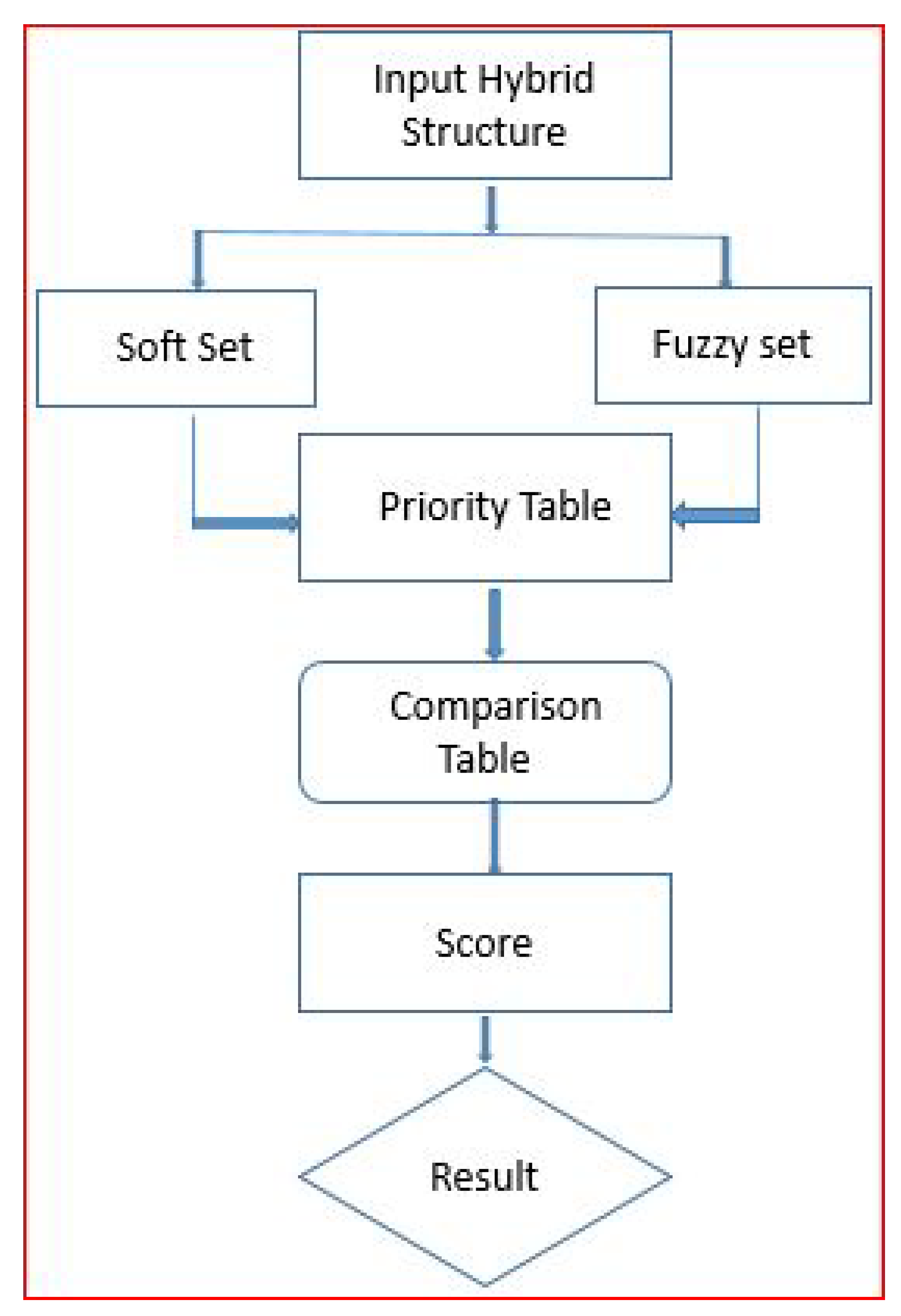
Step 1. Input the hybrid structure in tabular form (defined in Section 5.1). Step 2. Represent the tabular form of the soft set as given in [9] and fuzzy set in separate tables. Step 3. Construct the priority table (PT). This table can be achieved by multiplying the tabular values of the soft set with the corresponding values of the fuzzy membership of parameters. Also calculate the row sum of each row in priority table. Step 4. Construct the comparison table (CT) according to [42]. This can be achieved by finding the entries as differences of each row sum in priority table with those of all other rows. Step 5. Find the row sum of each row in the comparison table to obtain the score. Step 6. Finally, the highest score is chosen. |
The flowchart in Figure 1 summarizes the step-by-step process of the proposed algorithm and logical flow towards achieving its objectives.
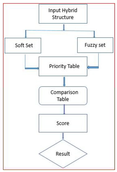
Figure 1.
Flow diagram of the proposed algorithm.
5.3. Example
To empirically evaluate the effectiveness of our proposed algorithm, we give an example of the selection of a school for a cochlear-implanted child from a real-life scenario. The decision of selecting a school for a child with a cochlear implant is a critical and common decision that parents of such children often face.
A cochlear implant is an electronic device that can provide partial hearing to individuals with severe to profound hearing loss. Advances in early identification, implant technology, and early intensive therapy have enabled the implanted child to study in mainstream schools. Visual distraction, background noise, or any other environmental sounds may interfere with the understanding speech for a child with an implant. So, the decision of the selection of a school for an implanted child is based on the individual needs of the child, their capacity to learn in a spoken language environment, the environment of the school, and cooperation of the teaching staff.
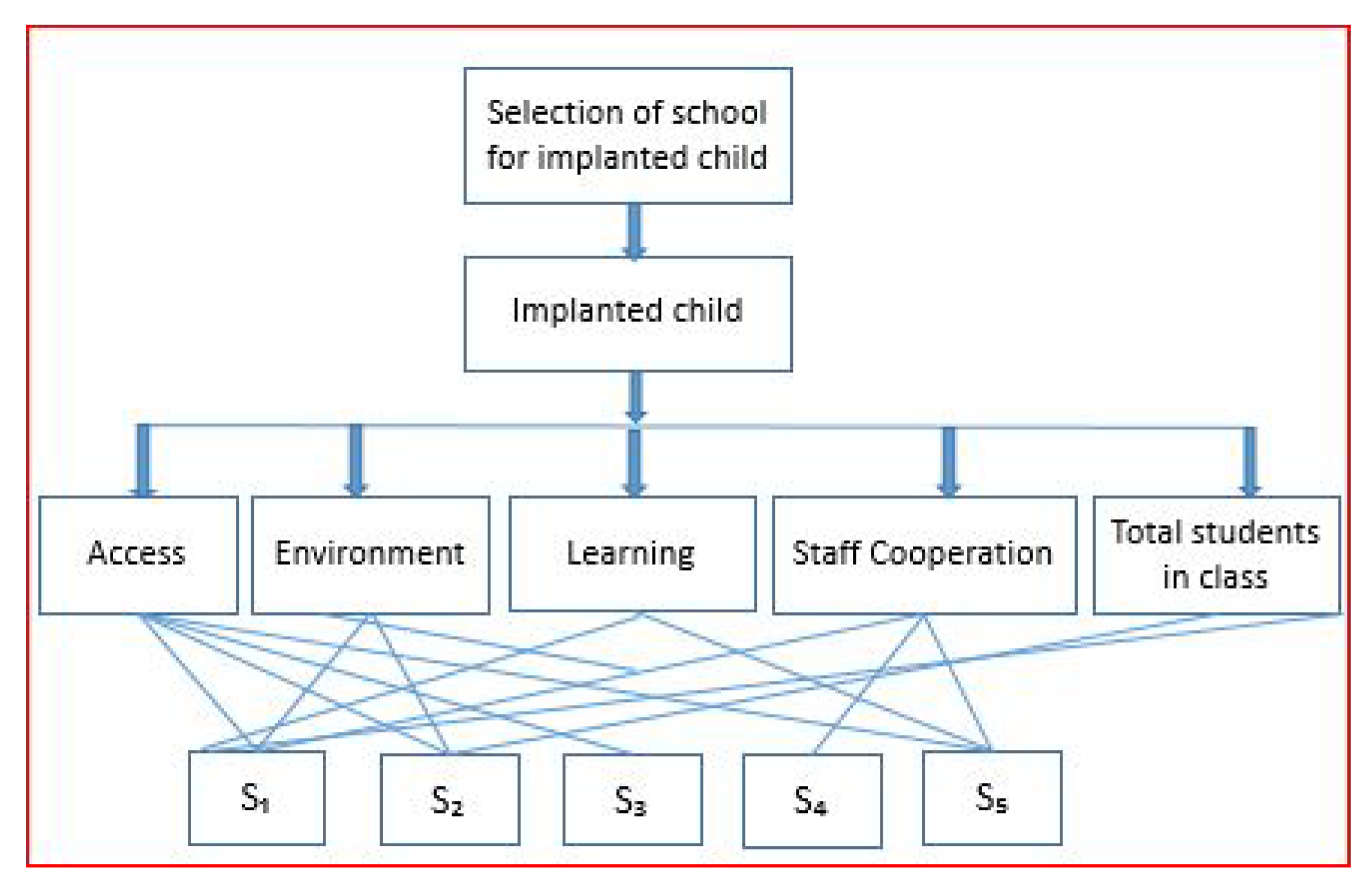
Suppose Mr and Mrs Ali are in search of a school for their implanted child. To complete this task, the parents visit some schools and collect the required information about different schools in their area. They choose the five schools, namely, “Beacon House” () “The city school” () “Pak-American” (), “Educators”(, and “Superior Montessori” ( who are willing to give admission to the child. The parents configure five attributes where “access” (),“environment” (), “learning” (), “staff cooperation” (), and “no of students in class” () as a set of parameters which they think are crucial for making the best option and ensuring their child’s adequate education. A hierarchical structure is shown in Figure 2, presenting the five selection criteria (i.e., access, environment, learning, staff cooperation, and the number of pupils in the class).
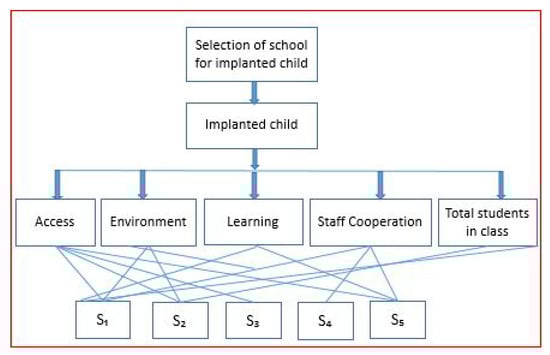
Figure 2.
Hierarchical structure for the selection of school for implanted child.
Based on these criteria, the family wants to select the best school. The following hybrid structure illustrates the information of the schools based on the chosen criteria.
We define the binary operation ⋄ and ∔ on by the Cayley table in Table 6.
Table 6.
Cayley tableof the binary operations ⋄ and ∔.
Then is a hemiring. For the implementation of our proposed Algorithm 1, the following steps are used.
Step 1: Based on the hybrid structure, all the possible values are estimated for the attributes, given in Table 7.
Table 7.
Tabular representation of hybrid structure.
Step 2. Construct seperate tables for the soft set and fuzzy set
Step 3. By multiplying the corresponding values of in Table 8 and in Table 9, Table 10 computes the priority table.
Table 8.
Tabular representation of .
Table 9.
Tabular representation of .
Table 10.
Priority table (PT).
Step 4. In Table 11, each attribute is obtained as the difference of row sum with the all the other rows.
Table 11.
Comprison Table (CT).
Step 5. Calculate the sum of each row in the comparison table to obtain the score of schools as shown in Table 12.
Table 12.
Score of alternatives.
Step 6. From the Table 12, we can see that alternative is the best selection.
Scores of alternatives for the selection of best school for implanted child are shown in Figure 3.
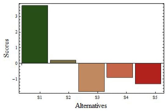
Figure 3.
Scores of alternatives for the selection of best school for implanted child.
In Figure 3, the bar chart serves as a visual representation of the alternative values derived from the evaluation criteria outlined in Table 12. The chart allows for a clear and concise comparison of the different schools (, , , , and ) based on their respective scores.
At the top of the bar chart, we can observe that Beacon House School () stands out with the highest score of 3.7 among all the schools. This score reflects its excellent performance in the evaluation criteria, indicating that it outperformed the other schools in the assessment.
The City School () follows closely behind Beacon House School, securing the second-highest score. This suggests that The City School is also a strong competitor and performed admirably in the comparison.
However, the alternatives at the bottom of the bar chart, namely The Pak-American School (), The Educators School (), and The Superior Montessori School (), obtained relatively lower scores. These scores indicate that these schools had comparatively lesser acceptability or performance based on the assessment criteria.
The bar chart, as an essential part of the decision-making process, provides a visual tool to discern the varying levels of performance among the alternatives. It simplifies the comparison, allowing decision-makers to identify the top-performing school (Beacon House School) and observe the relative positions of the other schools in terms of their scores.
By incorporating a bar chart into the decision-making process, the evaluation becomes more intuitive and accessible. Decision-makers can make well-informed choices by considering the graphical representation of the schools’ performance, facilitating a clearer understanding of their respective strengths and weaknesses based on the evaluation criteria. The visual comparison aids in selecting the most appropriate school that aligns with the decision-maker’s preferences and requirements.
As compared to Asmat et al. [40,41] our proposed method has assessed the hybrid structure in hemirings and investigated several properties of hybrid h-bi-ideals. The proposed prime hybrid h-bi-ideals are an extension of hybrid h-bi-ideals and we have investigated various aspects of hemirings. Also, this work has conducted a characterization of certain classes of hemirings based on these prime hybrid h-bi-ideals. Furthermore, we have utilized the hybrid structure in the decision-making process with the help of examples from real-world situations to explore new directions in algebraic development and tackle practical problems with improved uncertainty-handling abilities by utilizing hybrid structures in hemirings. Furthermore, our proposed method distinguishes itself from the existing literature by adopting a hybrid structure-based model rather than focusing solely on algebraic structures like BCK/BCI algebras and semigroups, as seen in previous studies [35,36,37,38,39].
6. Conclusions
In summary, the paper highlights the significance of hybrid structures in mathematical and decision-making domains. This study focuses on investigating the properties of hybrid h-bi-ideals within the context of hemirings. These hybrid h-bi-ideals include prime, strongly prime, semiprime, irreducible, and strongly irreducible. By employing the hybrid h-bi-ideals, the paper provides insightful characterizations of h-hemiregular and h-intra-hemiregular hemirings. This analysis contributes to a deeper understanding of the algebraic structures associated with these types of hemirings. To this end, we present a decision-making algorithm based on hybrid structures that has been successfully applied to solve a significant real-world problem. This showcases the effectiveness of the proposed approach in providing robust solutions in situations involving imprecise or uncertain data. The practical utility of the findings is demonstrated through the successful application of the proposed decision-making algorithm to solve real-world problems under imprecise conditions.
The proposed hybrid structure-based model empowers decision-makers in complex situations with uncertainty. It helps them understand uncertainties comprehensively and make effective choices in diverse scenarios. By using both crisp and fuzzy information, it improves decision outcomes in various domains. Also, the proposed algorithm considers both quantitative and qualitative information, enhancing the decision-making process and reducing risks.
On the contrary to this, defining membership functions for fuzzy and soft sets requires extensive domain knowledge, and interpreting dual representation demands specialized expertise, making implementation and maintenance of the approach more challenging. Additionally, gathering precise and accurate data, especially for subjective or qualitative information, can be difficult. The effectiveness of the proposed hybrid structures relies on sufficient and reliable data; in situations with scarce or unreliable data, their accuracy and effectiveness may be compromised.
However, in the future, the applicability of hybrid structures may be assessed in different algebraic structures including rings, semirings, and lattices, acquiring insightful knowledge into their adaptability and efficiency. To handle complex situational decisions with multiple objectives and criteria more successfully, one could combine these hybrid structures with multi-criteria decision-making methodologies. Furthermore, comparative studies between the existing models and hybrid structures could be considered to understand their respective strengths and limitations in various decision-making scenarios.
Author Contributions
Conceptualization, A.H. and A.K.; Software, A.H., A.K., N.F. and D.M.K.; Validation, N.F., D.M.K., R.A.R.B. and M.E.; Formal analysis, A.H., A.K. and R.A.R.B.; Investigation, A.K., N.F., D.M.K. and M.E.; Resources, A.H., N.F., D.M.K., R.A.R.B. and M.E.; Data curation, A.H., N.F., R.A.R.B. and M.E.; Writing—original draft, A.H.; Writing—review editing, A.K.; Visualization, N.F., D.M.K., R.A.R.B. and M.E.; Supervision, A.K.; Project administration, D.M.K. and M.E.; Funding acquisition, R.A.R.B. All authors have read and agreed to the published version of the manuscript.
Funding
The technical and financial support—The Ministry of Education and King Abdulaziz University, DSR, Jeddah, Saudi Arabia.
Data Availability Statement
Not applicable.
Acknowledgments
This research work was funded by Institutional Fund Projects under grant no. (IFPIP: 550-150-1443). The authors gratefully acknowledge the technical and financial support provided by the Ministry of Education and King Abdulaziz University, DSR, Jeddah, Saudi Arabia.
Conflicts of Interest
The authors declare no conflict of interest.
Appendix A
Example A1.
Suppose that there are six houses in the initial universe set given by = {}. Let a set of parameters = {,,,} be a set of status of houses in which stands for the parameter “beautiful”, stands for the parameter “cheap”, stands for the parameter “in good location”, stands for the parameter “in green surrounding". We define the binary operation ⋄ and ∔ on by the Cayley table in Table A1.
Table A1.
Cayley table for the binary operations ∔ and ⋄.
Table A1.
Cayley table for the binary operations ∔ and ⋄.
| ∔ | ⋄ | |||||||||
Then (,∔,⋄) is a hemiring. Let and be a any ḦyH-BI in over which is given by Table A2, Table A3 and Table A4.
Table A2.
Tabular representation of ḦyH-BI .
Table A2.
Tabular representation of ḦyH-BI .
| { | ||
Table A3.
Tabular representation of ḦyH-BI
Table A3.
Tabular representation of ḦyH-BI
Table A4.
Tabular representation of ḦyH-BI
Table A4.
Tabular representation of ḦyH-BI
It is a routine calculation to verify that if and implies or and or for all ,,, in This implies that ( gives or . Thus, is a strongly prime ḦyH-BI of over
Example A2.
Suppose that there are six houses in the initial universe set given by = {}. Let a set of parameters = {,,,} be a set of status of houses in which stands for the parameter “beautiful”, stands for the parameter “cheap”, stands for the parameter “in good location”, stands for the parameter “in green surrounding". We define the binary operation ⋄ and ∔ on by the Cayley table in Table A5.
Table A5.
Cayley table for the binary operations ∔ and ⋄.
Table A5.
Cayley table for the binary operations ∔ and ⋄.
| ∔ | ⋄ | |||||||||
Table A6.
Tabular representation of ḦyH-BI
Table A6.
Tabular representation of ḦyH-BI
| { | ||
Table A7.
Tabular representation of ḦyH-BI
Table A7.
Tabular representation of ḦyH-BI
It is a routine calculation to verify that if and implies and for all ,,, in This implies that ( gives . Thus, is a semiprime ḦyH-BI of over
References
- Zadeh, L.A. Fuzzy sets. Inform. Control 1965, 8, 338–353. [Google Scholar] [CrossRef]
- Zadeh, L.A. Fuzzy sets. Towards a generalized theory of uncertainity. Inf. Sci. 2005, 172, 1–40. [Google Scholar] [CrossRef]
- Debois, D.; Prade, H. Fuzzy Set and Systems: Theory and Applications; Academic Press: New York, NY, USA, 1990. [Google Scholar]
- Klir, G.J.; Folger, T.A. Fuzzy Sets, Uncertainity and Information; Printice Hall, Inc.: Hoboken, NJ, USA, 1968. [Google Scholar]
- Zimmerman, H.J. Fuzzy Set Theory and Its Applications; Acedemic Publishers: Cambridge, MA, USA, 1991. [Google Scholar]
- Pawlak, Z. Rough sets. Int. J. Inf. Comput. Sci. 1962, 11, 34–352. [Google Scholar]
- Gorzalzany, M.B. A method of inference in approximate reasoning based on interval-valued fuzzy sets. Fuzzy Sets Syst. 1987, 21, 1–17. [Google Scholar] [CrossRef]
- Molodtsov, D. Soft set theory-first results. J. Intell. Fuzzy Syst. 1999, 37, 19–31. [Google Scholar] [CrossRef]
- PMaji, K.; Biswas, R.; Roy, A.R. Fuzzy soft sets. J. Fuzzy Math. 2001, 9, 589–602. [Google Scholar]
- Majumdar, P.; Samanta, S.K. Generalised fuzzy soft sets. Comput. Math. Appl. 2010, 59, 1425–1432. [Google Scholar] [CrossRef]
- Yang, X.B.; Lin, T.Y.; Yang, J.Y.; Li, Y.; Yu, D.J. Combination of interval-valued fuzzy set and soft set. Comput. Math. Appl. 2009, 58, 521–527. [Google Scholar] [CrossRef]
- Roy, A.R.; Maji, P.K. A fuzzy soft set theoretic approach to decision making problems. J. Comput. Appl. Math. 2007, 203, 412–418. [Google Scholar] [CrossRef]
- Aktas, H.; Çagman, N. Soft sets and soft groups. Inf. Sci. 2007, 177, 2726–2735. [Google Scholar] [CrossRef]
- Feng, F.; Jun, Y.B.; Zhao, X.Z. Soft semirings. Comput. Math. Appl. 2008, 56, 2621–2628. [Google Scholar] [CrossRef]
- Jun, Y.B.; Park, C.H. Applications of soft sets in ideal theory of BCK/BCI-algebras. Inf. Sci. 2008, 178, 2466–2475. [Google Scholar] [CrossRef]
- Jun, Y.B.; Lee, K.J.; Zhan, J. Soft p-ideals of soft BCI-algebras. Comput. Math. Appl. 2009, 58, 2060–2068. [Google Scholar] [CrossRef]
- Jun, Y.B.; Lee, K.J.; Park, C.H. Fuzzy soft set theory applied to BCK/BCI-algebras. Comput. Math. Appl. 2010, 59, 3180–3192. [Google Scholar] [CrossRef]
- Jun, Y.B.; Lee, K.J.; Khan, A. Soft ordered semigroups. Math. Log. Q. 2010, 56, 42–50. [Google Scholar] [CrossRef]
- Jun, Y.B.; Song, S.Z.; So, K.S. Soft set theory applied to p-ideals of BCI-algebras related to fuzzy points. Neural Comput. Appl. 2011, 20, 1313–1320. [Google Scholar] [CrossRef]
- Zhan, J.; Jun, Y.B. Soft BL-algebras based on fuzzy sets. Comput. Math. Appl. 2010, 59, 2037–2046. [Google Scholar] [CrossRef]
- Ali, M.I. A note on soft sets, rough soft sets and fuzzy soft sets. Appl. Soft Comput. 2011, 11, 3329–3332. [Google Scholar]
- Liu, Z.; Qin, K.; Pei, Z. Method for Fuzzy Soft Sets in Decision-Making Based on an Ideal Solution. Symmetry 2017, 9, 246. [Google Scholar] [CrossRef]
- Rehman, U.U.; Mahmood, T. Picture Fuzzy N-Soft Sets and Their Applications in Decision-Making Problems. Fuzzy Inf. Eng. 2021, 13, 335–367. [Google Scholar] [CrossRef]
- Feng, F.; Jun, Y.B.; Liu, X.Y.; Li, L.F. An adjustable approach to fuzzy soft set based decision making. J. Comput. Appl. Math. 2010, 234, 10–20. [Google Scholar] [CrossRef]
- Qin, H.; Ma, X.; Wang, J. A Novel Approach to Decision Making Based on Interval-Valued Fuzzy Soft Set. Symmetry 2021, 13, 2274. [Google Scholar] [CrossRef]
- Khan, A.; Yang, M.; Haq, M.; Shah, A.A.; Arif, M. A New Approach for Normal Parameter Reduction Using σ-Algebraic Soft Sets and Its Application in Multi-Attribute Decision Making. Mathematics 2022, 10, 1297. [Google Scholar] [CrossRef]
- Henriksen, M. Ideals in semirings with commutative addition. Am. Math. Soc. Not. 1958, 6, 321. [Google Scholar]
- Iizuka, K. On Jacobson radical of a semiring. Tohoku Math. J. 1959, 11, 409–421. [Google Scholar] [CrossRef]
- LaTorre, D.R. On h-ideals and k-ideals in hemirings. Publ. Math. 1965, 12, 219–226. [Google Scholar] [CrossRef]
- Jun, Y.B.; Öztürk, M.A.; Song, S.Z. On fuzzy h-ideals in hemirings. Inform. Sci. 2004, 162, 211–226. [Google Scholar] [CrossRef]
- Zhan, J.; Dudek, W.A. Fuzzy h-ideals of hemirings. Inform. Sci. 2007, 177, 876–886. [Google Scholar] [CrossRef]
- Yin, Y.; Li, H. The characterizations of h-hemiregular hemirings and h-intra-hemiregular hemirings. Inform. Sci. 2008, 178, 3451–3464. [Google Scholar] [CrossRef]
- Anjum, R. Some Studies in Fuzzy Hemirings. Ph.D. Thesis, Department of Mathematics, Quaid-i-Azam University, Islamabad, Pakistan, 2011. [Google Scholar]
- Anis, S.; Khan, M.; Jun, Y.B. Hybrid ideals in semigroups. Cogent Math. 2017, 4, 1352117. [Google Scholar] [CrossRef]
- Jun, Y.B.; Song, S.Z.; Muhiuddin, G. Hybrid structures and applications. Ann. Commun. Math. 2018, 1, 11–25. [Google Scholar]
- Muhiuddin, G.; Kadi, D.A.; Mahboob, A. Hybrid structures applied to ideals in BCI-Algebras. J. Math. 2020, 2020, 2365078. [Google Scholar] [CrossRef]
- Muhiuddin, G.; Kadi, D.A.; Mahboob, A. Ideal theory of BCK/BCI-Algebras based on hybrid structures. J. Math. Comput. Sci. 2021, 23, 136–144. [Google Scholar] [CrossRef]
- Elavarasan, B.; Porselvi, K.; Jun, Y.B. Hybrid generalized bi-ideals in semigroups. Int. J. Math. Comp. 2019, 14, 601–612. [Google Scholar]
- Elavarasan, B.; Jun, Y.B. Regularity of semigroups in terms of hybrid ideals and hybrid bi-ideals. Kragujev. J. Math. 2022, 46, 857–864. [Google Scholar] [CrossRef]
- Hadi, A.; Khan, A.; Jun, Y.B. Hemirings characterized by their hybrid h-ideals. Bull. Sect. Log. 2022, 3, 100–112. [Google Scholar]
- Khan, A.; Hadi, A.; Ibrar, M.; Jun, Y.B. Hybrid structures applied to hemirings. J. Intell. Fuzzy Syst. 2019, 37, 4873–4889. [Google Scholar] [CrossRef]
- Tripathy, B.K.; Sooraj, T.R.; Mohanty, R.K. A New Approach to Fuzzy Soft Set Theory and Its Application in Decision Making. In Computational Intelligence in Data Mining—Volume 2: Proceedings of the International Conference on CIDM, 5–6 December 2015; Springer: New Delhi, India, 2016. [Google Scholar]

Disclaimer/Publisher’s Note: The statements, opinions and data contained in all publications are solely those of the individual author(s) and contributor(s) and not of MDPI and/or the editor(s). MDPI and/or the editor(s) disclaim responsibility for any injury to people or property resulting from any ideas, methods, instructions or products referred to in the content. |
© 2023 by the authors. Licensee MDPI, Basel, Switzerland. This article is an open access article distributed under the terms and conditions of the Creative Commons Attribution (CC BY) license (https://creativecommons.org/licenses/by/4.0/).