Abstract
Transformer-based graph neural networks have accomplished notable achievements by utilizing the self-attention mechanism for message passing in various domains. However, traditional methods overlook the diverse significance of intra-node representations, focusing solely on internode interactions. To overcome this limitation, we propose a DAG (Dual Attention Graph), a novel approach that integrates both intra-node and internode dynamics for node classification tasks. By considering the information exchange process between nodes from dual branches, DAG provides a holistic understanding of information propagation within graphs, enhancing the interpretability of graph-based machine learning applications. The experimental evaluations demonstrate that DAG excels in node classification tasks, outperforming current benchmark models across ten datasets.
MSC:
68T07
1. Introduction
Graph neural networks (GNNs) have gained widespread recognition as strong tools for solving real-world problems in diverse domains. They have been successfully applied in recommendation systems [1,2,3,4], bioinformatics [5,6,7], traffic prediction [8,9,10], natural language processing [11,12], drug discovery [13,14,15], fraud detection [16,17,18], robotics [19,20,21], and social media analysis [22,23], among other fields. The effectiveness of current GNNs can be attributed to their utilization of techniques such as gated recurrent units and the self-attention mechanism. These techniques enable GNNs to recursively aggregate information along edges and update features on the center node. By employing a message-passing mechanism, GNNs effectively learn from graph-structured data and make accurate predictions. This ability to capture and propagate information across the graph enables GNNs to tackle various challenges and provide valuable insights into different application domains.
In the early stages of GNNs [24,25], a common approach involved using a uniform message-passing strategy to handle all nodes. However, this approach failed to consider the significance of node attributes, resulting in the potential disregarding of important information. Consequently, the performance of models relying on this strategy could be negatively impacted. The uniform message-passing strategy did not effectively leverage the rich information contained in node attributes, limiting the ability of the GNNs to capture intricate patterns and dependencies within graphs. As a result, there is a need to overcome this limitation and develop approaches that could better utilize both the node attributes and graph structure to improve performance in various tasks.
To address the limitations of the traditional uniform message-passing strategy, attention-based GNN methods have been introduced [26,27]. These methods aimed to evaluate the contribution of neighboring nodes to the central node, enabling more effective utilization of graph information. By assigning varying degrees of importance to different nodes, attention-based methods could better capture the relevance and significance of node attributes during information propagation. This allowed the model to focus on relevant information and make more informed decisions. By considering the features of neighboring nodes in updating a node’s attributes, attention-based methods accounted for the individual contributions of nodes in the overall information transmission. This approach enhanced the representation and information flow within GNNs, leading to enhanced accuracy in tasks such as node classification and prediction.
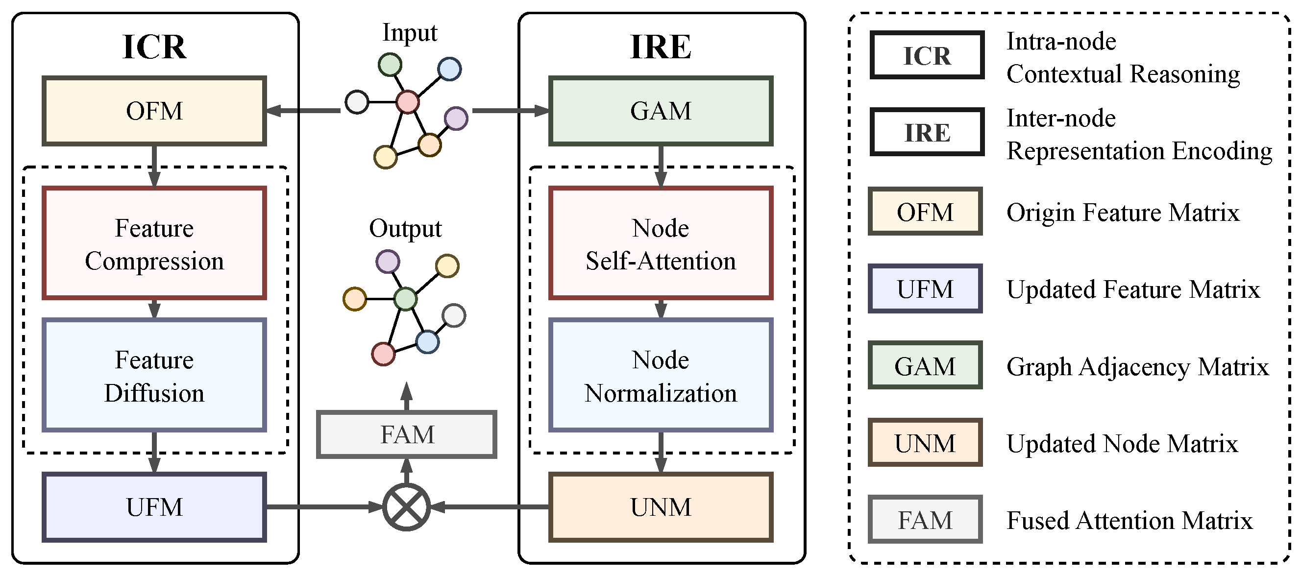
Building upon the progress made with attention-based GNN methods, we propose a novel method called Dual Attention Graph Representation Learning (DAG). The DAG approach addresses the limitations of the traditional uniform message-passing strategy by considering both the link relationships among nodes and the attributes of the nodes themselves. We can consider a graph as a structure composed of nodes and their connections. Traditional approaches may only focus on the link relationships between the nodes while neglecting the attributes of the nodes themselves. However, in complex real-world graphs, the attributes of the nodes are also crucial, as they can serve as auxiliary features to provide additional information for a more comprehensive analysis and interpretation of the graph’s structure and meaning. Therefore, we leverage a dual branch mechanism to comprehend both intra-node and internode dynamics, enabling a more comprehensive understanding of the information propagation within graphs, as shown in Figure 1. The Internode Representation Encoding (IRE) branch analyzes the differences between nodes on the graph and examines the contribution of neighboring nodes. On the other hand, the Intra-node Contextual Reasoning (ICR) branch explores the individual node attributes and dynamically updates the feature matrix of the graph nodes based on the current node category. By combining these two branches, DAG facilitates more effective information propagation and enhances the node classification performance. The proposed DAG approach offers a promising direction for advancing graph representation learning and improving the capabilities of GNNs in various applications.
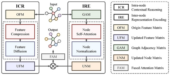
Figure 1.
Upon receiving the input graph, the Dual Attention Graph representation learning (DAG) employs two concurrent procedures, namely IRE and ICR, to investigate the representation conveyed via intra- and internodes on the graph. The IRE procedure focuses on the analysis of the structural information among the interconnected nodes, while the ICR procedure delves into the internal representations within each node. The detail of the ICR is shown in Figure 2.
The proposed DAG offers several key advantages over traditional uniform message-passing strategies and attention-based methods. Firstly, the DAG explicitly considers the impact of both the link relationships between nodes and the features of the nodes themselves on the task at hand. By incorporating intra-node and internode dynamics, the DAG provides a more comprehensive and holistic understanding of information propagation within graphs. This enables the model to capture intricate patterns and dependencies, leading to improved performance in tasks such as node prediction and classification. Secondly, the dual branch mechanism in the DAG allows for the simultaneous exploration of both the semantic information within individual nodes and the structural information among neighboring nodes. This combination enables DAG to leverage the strengths of both types of information, enhancing the model’s ability to gather both local and global context in the graph. Finally, the dynamic feature update process in the DAG ensures that the representation of each node is adaptively adjusted based on its current category, facilitating more accurate and informative feature representations. Through extensive experimental evaluations on ten different scalable graph datasets under node classification tasks, the DAG consistently demonstrated outstanding performance, surpassing existing approaches and showcasing its effectiveness and potential for advancing graph representation learning in various real-world applications. The versatility and superior performance of DAG make it a promising framework for addressing complex graph-based problems in diverse domains.
This paper presents the following contributions:
- This paper introduces DAG, a novel approach that addresses the limitations of traditional uniform message-passing strategies and attention-based methods in graph neural networks. The DAG incorporates both intra-node and internode dynamics, considering the link relationships between the nodes and the features of the nodes themselves. This dual attention mechanism enables DAG to capture rich information propagation patterns within graphs, leading to improved accuracy in tasks such as node prediction and classification.
- The proposed DAG offers a holistic and comprehensive exploration of both the semantic information within individual nodes and the structural information among neighboring nodes. By leveraging the strengths of both types of information, the DAG enhances the model’s ability to capture the local and global context within the graph. This comprehensive exploration contributes to more accurate and informative feature representations, improving the overall performance of graph-representation-learning tasks.
- Extensive experimental evaluations on ten different scalable graph datasets prove the outstanding performance of the DAG. The proposed approach consistently outperforms existing methods, showcasing its effectiveness in various practical scenarios. The outstanding performance of the DAG reaffirms its potential for advancing graph representation learning, providing valuable insights into information propagation dynamics within graphs, and facilitating more accurate and interpretable predictions.
2. Related Work on Graph Neural Networks
GNNs have gained significant attention in recent years due to their capacity for handling data with a graph-based structure. Numerous methods have been suggested to tackle the challenges of information aggregation and representation learning in GNNs. This section covers three significant research areas that are relevant to our work: aggregation operations on graphs, attention mechanisms in GNNs, and advanced techniques in graph representation learning.
2.1. Aggregation Operations on Graphs
Aggregation operations play a crucial role in GNNs by capturing information from neighboring nodes. One widely used method is the Graph Convolutional Network (GCN) [28], which aggregates information by determining the weighted sum of the neighboring node features. The GCN has demonstrated promising results in diverse applications, such as node classification and link prediction tasks. Other aggregation techniques include GraphSAGE [29], which employs sampling and layer-wise aggregation functions, and ChebNet [30], which uses graph spectral filters for information propagation. Additionally, Diffusion Convolutional Neural Networks (DCNN) [31] leverage heat diffusion processes to model information flow on graphs.
2.2. Self-Attention Mechanisms in GNNs
Attention mechanisms have been widely adopted in GNNs to calculate the importance weights for nodes in the graph. Graph Attention Networks (GAT) [32] introduced self-attention mechanisms that allow nodes to selectively attend to informative neighbors. Other attention-based methods include Graph Isomorphism Networks (GIN) [33], which employ global pooling and multilayer perceptrons to aggregate information, and Graph Transformer Networks (GTN) [34], which adapt the transformer architecture for graph data. These attention-based models enhance the ability of GNNs to capture complex relationships and focus on relevant features during information propagation.
2.3. Advanced Techniques in Graph Representation Learning
Beyond traditional aggregation operations and attention mechanisms, several advanced techniques have been proposed for graph representation learning. GraphSaint [35] addresses the scalability issue by introducing graph sampling techniques to select informative subgraphs for training. GraphWave [36] combines graph wavelet transforms with deep learning models to capture the multiscale structural information. Graph Contrastive Learning (GraphCL) [37] methods leverage contrastive learning frameworks to learn effective node and graph representations. Graph Autoencoders (GAE) [38] employ encoder–decoder architectures for unsupervised representation learning. GaAN [39] incorporates a convolutional subnetwork.
Overall, while existing approaches have made significant contributions to graph representation learning, they still face challenges in effectively capturing long-range dependencies and incorporating the importance of internal feature relationships. In our work, we introduce a novel method that addresses these limitations by explicitly considering both local and global information exchange in a dual attention framework. By combining the strengths of aggregation operations, attention mechanisms, and advanced techniques, we aim to enhance the representation learning capabilities of GNNs for improved performance in various graph-based applications.
3. Methods
The goal of the DAG is to enhance information propagation and representation learning on static graphs by incorporating both intra-node and internode dynamics. The DAG aims to enhance the accuracy of the node classification and prediction tasks by capturing intricate patterns and dependencies within graphs. As depicted in Figure 1, the proposed DAG is designed to capture the relationships and features between nodes in graph data through its unique architecture, which incorporates the Internode Representation Encoding (IRE) and Intra-node Contextual Reasoning (ICR) modules. The IRE module quantifies the impact of surrounding nodes on the central node by learning the Updated Node Matrix (UNM) and capturing the structural information within the graph. Simultaneously, the ICR module emphasizes node-specific attributes and contextual information by learning the Updated Feature Matrix (UFM). By combining the UNM and UFM, the DAG generates a Fused Attention Matrix (FAM) that integrates internode relationships and intra-node features. This comprehensive attention mechanism enables DAG to effectively capture complex dependencies and patterns, ultimately facilitating accurate node classification predictions.
With its architecture leveraging the IRE and ICR modules, the DAG offers a holistic understanding of graph data by capturing both internode relationships and intra-node features. The IRE module accounts for the collective impact of neighboring nodes, while the ICR module focuses on the unique attributes of each node. By integrating these modules, the DAG achieves a comprehensive representation of the graph that considers both its structural properties and attribute information. This integration enables the DAG to capture intricate dependencies within the graph, resulting in improved performance in node classification tasks. The effective fusion of internode and intra-node information sets the DAG apart as a powerful approach for graph representation learning, providing a more nuanced and comprehensive understanding of graph data.
3.1. Internode Representation Encoding
The graph adjacency matrix (GAM) is a widely used representation of node relationships in graphs, providing insights into the graph’s structure and features. However, the GAM has limitations in effectively incorporating the influences of multiple adjacent vertices on a target vertex [40]. To overcome this limitation, attention-based methods like GTN have emerged. Inspired by the GTN, we introduce IRE as a novel approach to capture the influence of each adjacent node on the central node.
The IRE consists of three key operations. Firstly, we propose a self-attention mechanism to the graph adjacency matrix, allowing the model to dynamically assign weights to the relationships between nodes based on their importance. This mechanism enables the model to focus on more relevant node relationships during the message-passing process. Secondly, we perform node normalization on the updated graph feature matrix, ensuring that the features of each node are appropriately scaled and weighted. This normalization step enhances the comparability and interpretability of nodes. Finally, we update the node representations by aggregating information from the neighboring nodes toward the center node. This process captures the relevant information from the adjacent nodes, enriching the representation of the central node.
By incorporating these three operations, the IRE enhances the representation of node relationships in graphs and addresses the limitations of the graph adjacency matrix. It enables the model to allocate weights to node relationships according to their importance, normalize node features, and update node representations through message passing. This comprehensive approach provides a more precise and informative representation of the relationships and features between nodes, facilitating improved understanding and analysis of complex graph data.
3.2. Intra-Node Contextual Reasoning
In the process of node information propagation in GNNs, nodes first aggregate the information of their neighboring nodes according to certain rules and weights and then update their own feature representation using the collected information. However, since all nodes have the same priority during the message aggregation process, this may result in some nodes transmitting useless information or even interfering with the efficient transmission of important information. Assigning priority to the representation of all graph node features can effectively solve this issue, but it also leads to a notable rise in computational complexity.
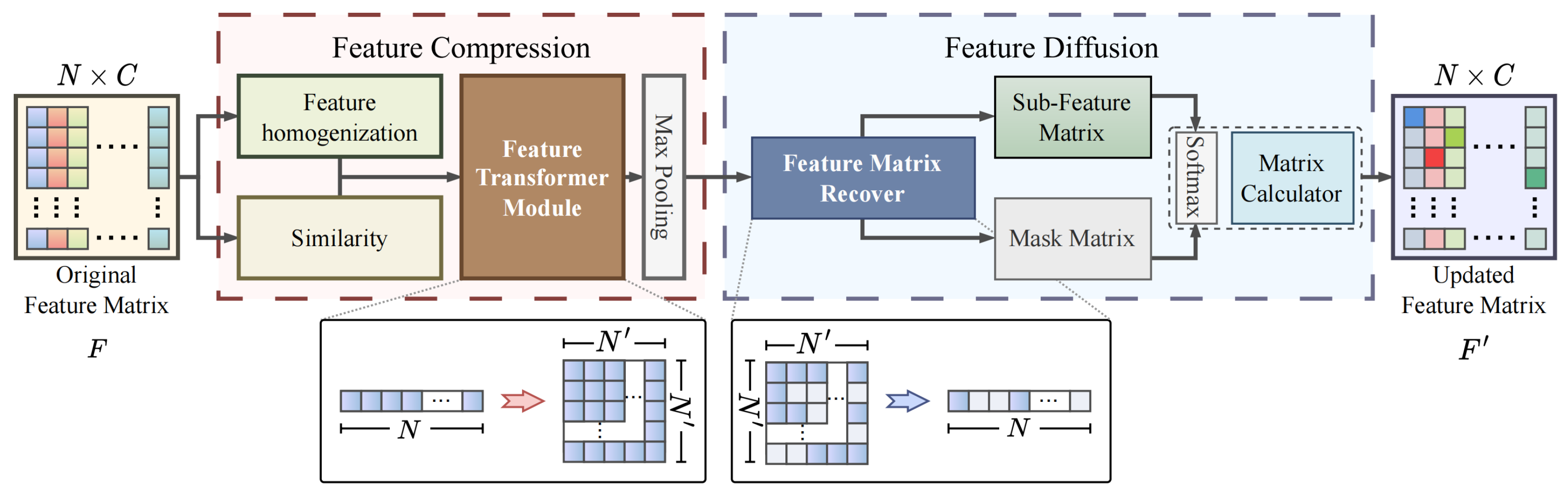
To handle this challenge, we propose a self-attention mechanism to compute the priority of features from nodes of different categories. This mechanism utilizes self-attention to evaluate the dependency weights between nodes in an adaptive manner, thereby capturing the differences in importance between them. Additionally, since the mechanism focuses solely on information relevant to the current node, it can reduce the computational complexity and enhance the information transmission efficiency. The ICR consists of two modules connected in series: Feature Compression (FC) and Feature Diffusion (FD). The FC module acts as a filtering mechanism that retains the most significant characteristics in the feature map and simultaneously reduces its size to enhance the computational efficiency. Meanwhile, the FD module discriminates between the significance of different attributes based on their categorical distinctions and ascertains their respective weights in the node representation.
3.2.1. Feature Compression Module
The FC module is designed to effectively process the node attributes by identifying the most representative features while minimizing the influence of the irrelevant attributes. This is crucial in node classification tasks, as it enables the discovery of interrelationships and similarities among attributes. Determining the correlation among all node attributes using an idealized approach is computationally expensive. It has a time complexity of , where N represents the number of nodes, and C represents the dimension of the input features. Due to the significantly increased computational burden compared to small graphs, large graphs, such as bioinformatics and recommendation systems, are limited in their applicability.
To address this challenge, the FC module aims to balance the investigation requirements and to categorize computations more efficiently. It leverages the category-oriented feature attention coefficients to assign weightings to the attributes in the node representation. This prioritizes the transmission of the most significant attributes along the edges of the graph within each category, while suppressing less relevant attributes. Importantly, the computational complexity of the FC module primarily depends on the overall number of node categories. By distinguishing and representing nodes of the same category using a single cascaded attention matrix, the computation can be greatly simplified to .
The FC module consists of three main operations as illustrated in Figure 2. Firstly, nodes in each sub-feature matrix are sorted to determine their importance within the category. Next, the sorted matrix is transformed into a three-dimensional sub-feature map, capturing the local salient features of each category. Finally, the FC module highlights the crucial local attributes of each node category, contributing to improving accuracy in node classification. By compressing and selectively emphasizing the relevant features, the FC module effectively reduces the computational complexity while preserving the essential information for accurate node classification.
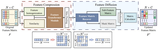
Figure 2.
The ICR can be divided into two interconnected sequential modules, FC and FD, which are presented separately in the red dashed box and the blue dashed box.
Feature homogenization. Feature homogenization is one approach to capture the similarities between nodes within a group or submatrix. It involves using the mean feature vector to represent a particular category, which promotes consistency and reduces noise. Once the common attribute vector for each category is established, the nodes within each submatrix can be sorted based on their proximity to the common attribute vector. This sorting method helps to identify patterns and relationships within the submatrix, making the data easier to analyze and interpret. Equation (1) compares each node’s feature vector against the average values of all the nodes’ features, in order to quantify the level of feature homogenization between them.
where is the cosine function, and the mean feature vector is calculated based on the average of all feature vectors within each category in the i-th sub-feature matrix. The sub-feature matrix comprises individual feature vectors represented by , which are utilized for computing the similarity, , between any pair of feature vectors.
Feature Transformer Module. Given that adjacent nodes in the sorted sub-feature matrices typically exhibit similar attributes, our main objective is to determine the most suitable attributes for each dimension C in the sorted 2D sub-feature matrix and allocate local advantage values to these attributes. C also represents the depth of the 3D feature map. To accomplish this objective, we transform into a matrix, where the is the number of feature vectors of the i-th sub-feature matrix. It is worth noting that this number is not always an integer. Therefore, in order to obtain an integer value for , it is necessary to round up to the nearest integer, where .
Max Pooling. In the last stage of the FC, we aim to identify the local dominant and representative attributes within each feature map and associate them with their corresponding category. To achieve this, we perform max pooling to downsample the feature maps and capture the most prominent features of each node category. The resulting feature maps, , are updated according to Equation (2) to obtain their new dimensions, .
The stride value, denoted by S, can effectively capture the intrinsic properties of each node category, which are crucial for accurately calculating the internal priority of the nodes in the FD module. The selection of this important feature plays a vital role in balancing the computation cost and performance. As excessively large stride values can reduce the computation burden but may also degrade the performance, excessively small stride values can result in prohibitively large computational burdens.
3.2.2. Feature Diffusion Module
Although the FC can highlight the most important features in each category, the priority between categories remains unknown. Therefore, the main goal of the FD is to determine the priority level of the crucial attributes in different categories, in order to classify the nodes more accurately. To achieve this objective, the FD adopts a sequential module approach, which includes two main steps: restoring the size of the 3D sub-feature map and transforming it back to a 2D sub-feature matrix, computing the internal priority. The specific details are shown in Figure 2.
Feature Matrix Recover. The first stage of the FD module involves restoring the feature maps to their original size. To achieve this, we use upsampling to recover the reduced feature map. The feature maps are restored from to . Then, we fill all the missing pixels with zero values, which has no impact on the semantic information contained in the feature maps. Next, the feature maps are reshaped into a sub-feature matrix with reduced dimensions during the transformation process for further computation. To classify the nodes, the sub-feature matrix is sorted according to the original order of the nodes. A matching mask is generated with the same shape as the matrix, which records whether each node in its corresponding category has representative attributes (true/false). This enables the FD module to determine the priority of the most important feature across different categories.
Matrix Calculator. The module employs a self-attention mechanism with learnable parameters to each updated feature matrix using Equation (3) to calculate the prioritization of nodes within each category. This scheme identifies the most important nodes in each category and assigns them higher priority for further processing.
where and indicate the attention coefficient and vector of k-th dimension in each sub-feature matrix, respectively. We use masks to record the positions of the key features of the nodes, in order to reduce the computational resource consumption. Then, we activate the feature of the new nonlinear node t using Equation (4).
The final step of this process is to obtain an attention matrix from each of the two branches separately in Equation (5).
where represents the weights that can be adjusted during the learning process. Meanwhile, and are the activation functions used for the ICR and IRE, respectively. In this context, the variable denotes the representation of the center node, t, while m is one of the neighbor nodes, denoted as , associated with t. The representations of node m are denoted as . The indicates the significance assigned by node t to its neighboring node m. In the final process, the attention matrix obtained through combination contains both the graph structure information and the node-specific information. Algorithm 1 summarizes the ICR algorithm.
| Algorithm 1: the algorithmic flow of the Intra-node Contextual Reasoning |
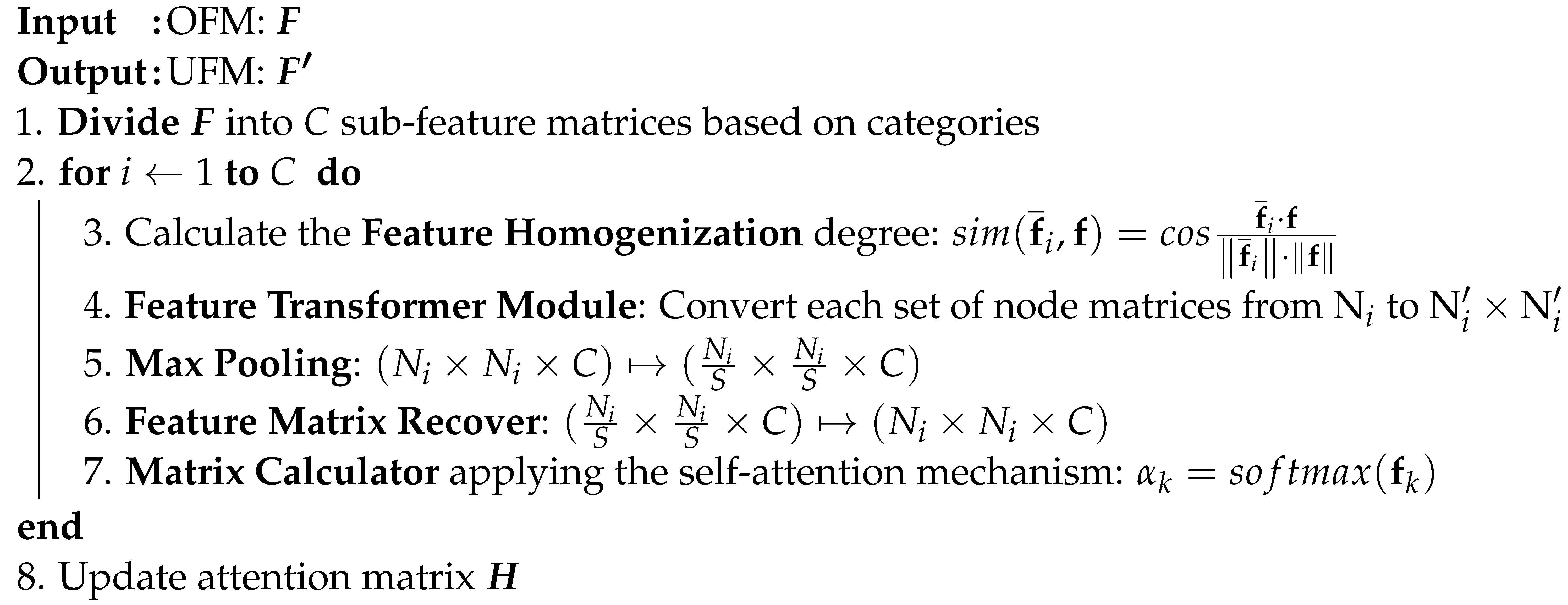 |
4. Experiments
4.1. Datasets
We evaluated the DAG method on ten commonly used graph datasets, including three homophily graph datasets, three heterophily graph datasets, two co-purchase datasets, and two coauthor graphs. Homophily refers to the tendency of connected nodes in a graph to exhibit similar characteristics or attributes. This similarity can be observed through nodes having identical labels or labels that are closely related. We used the homophily ratio [41] to distinguish subsets of the dataset. The homophily ratio denotes the proportion of edges connecting nodes with identical labels among the total number of edges. If this ratio was close to 1, we classified the dataset as a homophily graph dataset. Conversely, if the ratio was close to 0, we classified the dataset as a heterophily dataset [42]. The number of nodes, edges, features, and classes for each dataset are shown in Table 1.

Table 1.
Description of the graph datasets under the node classification task.
Cora, Citeseer [43], and PubMed [44] are three frequently utilized citation network datasets. In these undirected graphs, each node corresponds to a research paper, and the edges denote the citation connections between two papers. In these datasets, the task is to perform multiclass classification, where the objective is to assign a category to each node based on its corresponding field of study label. The node features are word vectors, where each element is a binary variable (0 or 1) indicating whether specific words are present in the corresponding paper. These datasets are commonly used for testing and comparing different graph-based learning algorithms and models, particularly in tasks such as node classification and prediction. Since the homophily ratio of these datasets was close to 1, we categorized them as homophily datasets.
Cornell, Chameleon, and Texas [45] are all web datasets. Cornell and Texas are the web datasets acquired by Carnegie Mellon University from these two universities. The dataset consists of connections between web pages, which are depicted as linked entities, with each connection symbolizing the relationship between them. Chameleon is a web page dataset of one of the topics in Wikipedia, which is composed of articles from Wikipedia, with each article being connected to others through hyperlinks. These connections serve as pathways for users to navigate between the articles, and the features represent the key information in the articles. Since the homophily ratio of these datasets was close to 0, we categorized them as heterophily datasets.
Coauthor CS and Coauthor Physics [46] are collaborated datasets representing researchers in computer science and physics-related fields, respectively. In these datasets, the coauthor datasets are composed of a collection of nodes representing authors, connected by edges that capture the collaborative relationships between them. These datasets have found extensive applications in fields such as deep learning and graph analysis to test and compare different graph learning algorithms and models.
Amazon Photo and Amazon Computers [47] are datasets representing co-purchasing patterns on the Amazon website. Each node in the graph represents a different product category, and each edge represents a bundled sales interest between two categories. The features associated with each node are obtained through a bag-of-words representation of customer reviews, where each feature vector dimension corresponds to the frequency of a particular word in the review. Amazon Computers is a binary classification task with positive or negative review labels, while Amazon Photo is a multiclass classification task with labels indicating the camera or photo category. These datasets are widely used for testing and comparing the graph learning algorithms and models, especially in recommendation systems.
4.2. Experimental Setup
We developed our model using the PyTorch framework and conducted training on four NVIDIA GeForce RTX 3090 GPUs. To prevent potential gradient vanishing or exploding issues during training, we initialized the parameters of our DAG model using the Xavier method, as detailed by Glorot et al. [48]. Following the completion of both the IRE and ICR procedures, we incorporated Exponential Linear Units (ELUs) [49] to yield nonlinear outcomes. For the final node classification tasks within the DAG network, a softmax layer [50] produced the probability distribution. To mitigate overfitting, dropout [51] was applied consistently throughout the model’s learning phase. The dropout rate ranged from to , depending on the specific dataset in use, and our graph feature pool was set at a size of two. For optimization, we utilized the AdamW optimizer combined with a cosine annealing approach, commencing with a learning rate of 0.02 and a weight decay of 0.05, spanning 300 epochs.
4.3. Comparison on Homophily Graph Datasets
To evaluate the effectiveness of our DAG, we first compared its results on identical datasets with other advanced techniques available in the field. Table 2 displays the accuracy of different methods for node classification on three homophily citation graphs. Previous studies have explored attention-based methods such as GraphStar [52], GraphNAS [53], and DIFNET [54], which leverage attention mechanisms to capture node features and have demonstrated strong performance on graph citation datasets. Non-attention-based methods, including Cleora [55] and 3ference [56], have also shown promising results. Additionally, Graph Decipher (GD) [40], which primarily focuses on node classification in imbalanced multiclass graph datasets, stands out due to its ability to investigate category-specific features by exploring representative node attributes.
Table 2.
Comparison with the most advanced approaches for node classification on three homophily graph datasets. We use the color green to signify a decrease in performance and the color red to represent an improvement. The optimal results (Accuracy) are highlighted in bold.
Despite the continuous improvement in the most advanced methods, our DAG method exhibited competitive performance. As indicated in the table, DAG achieved a performance that was only 1.6% lower than the best method on the PubMed dataset. Notably, on both the Cora and Citeseer datasets, DAG outperformed the second-ranked GD method by a margin of 1.2%. The results of the experiments confirm that our DAG approach effectively leverages the inherent structure and features of citation graphs for accurate node classification. By incorporating category-related node features, the DAG exhibits comparable performance to the best method on the PubMed dataset and outperforms other approaches on the Cora and Citeseer datasets. These results also demonstrate the effectiveness of DAG as a valuable graph-based approach for node classification tasks, specifically on homophily graph datasets.
4.4. Comparison on Heterophily Graph Datasets
In order to further examine the effectiveness of DAG on heterophily graph datasets, we evaluated our approach using three distinct datasets, which were Cornell, Chameleon, and Texas. Seven representative approaches were selected in addition to the DAG for comparative analysis, as shown in Table 3. Geom-GCN [57] extracts more structural information from the graph, where nodes that are far apart in the original graph are transformed into neighboring nodes in the latent space to facilitate information propagation. SDRF [58] proposes a node classification method based on an edge-based combined curvature. CNMPGNN [59] introduces the concept of common neighbors, while GGCN [60] learns node weights by simultaneously considering both the structural and feature edges. FDGATII [61] adopts dynamic attention to preserve key feature information in the graph. GloGNN [62] achieves group-wise optimization by gathering information from all nodes present in the graph.
Table 3.
Comparison with the most advanced approaches for node classification on three heterophily graph datasets. We use red to indicate performance improvement. The optimal results (Accuracy) are highlighted in bold.
From the table, we can see clearly that the DAG achieved accuracy rates of 88.49%, 74.16%, and 88.18% on the three datasets, respectively. Compared to the second-ranking method GD, DAG outperformed it by 1.23%, 1.69%, and 1.45%, respectively. These results demonstrate that the DAG can effectively capture both the node properties and the impact of their neighboring nodes within the graph structure, playing a critical role in node classification tasks. Meanwhile, these experiments also validate that our DAG method exhibits outstanding performance on heterophily graph datasets.
4.5. Comparison on More Graph Datasets
In addition, we evaluated our method on four more graph datasets, including two Coauthor graphs and two co-purchase datasets, and compared it with seven other methods, as shown in Table 4. It can be observed that the MLP, the only non-GNN method, performed relatively poorly. On the other hand, MoNet, GCN, GraphSAGE, GAT, and GD [28,29,32,40,63] all considered the mechanism of information propagation between nodes in the graph. They achieved significantly higher accuracy rates on all four datasets, especially Graph Decipher, which achieved accuracy rates of 95.9%, 97.3%, 83.1%, and 89.3%, respectively. However, it can also be observed that the GAT performed poorly on Amazon Computers and Amazon Photo, with accuracy rates of only 78.0% and 85.1%, respectively. This is because the GAT solely focuses on the impact of neighboring nodes on the central node, neglecting other factors that may also affect the node’s characteristics, resulting in a slightly worse performance on these two graph datasets with more complex and diverse node relationships.
Table 4.
Comparison with the most advanced approaches for node classification on more graph datasets. We use red to indicate performance improvement. The optimal results (Accuracy) are highlighted in bold. CC: Coauthor CS; CP: Coauthor Physics; AC: Amazon Computers; AP: Amazon Photo.
This finding emphasizes the superiority of GNNs in capturing and leveraging both local node features and the interconnections among nodes. The message-passing mechanism employed by GNNs facilitates the propagation of information through the graph, enabling a comprehensive understanding of the network structure and enhancing the representation learning process. By considering the context and relationships within the graph, GNNs can effectively capture the nuanced patterns and dependencies present in the data, improving classification performance.
Therefore, we propose further innovation by not only considering the relationships between nodes in GNN but also fully considering the influence of node attributes. By employing this technique, we obtained the best accuracy on four datasets, achieving 96.4%, 98.2%, 84.3%, and 92.0% accuracy, respectively. In summary, these experiments once again demonstrate the effectiveness of the DAG.
4.6. Effectiveness of the IRE and ICR
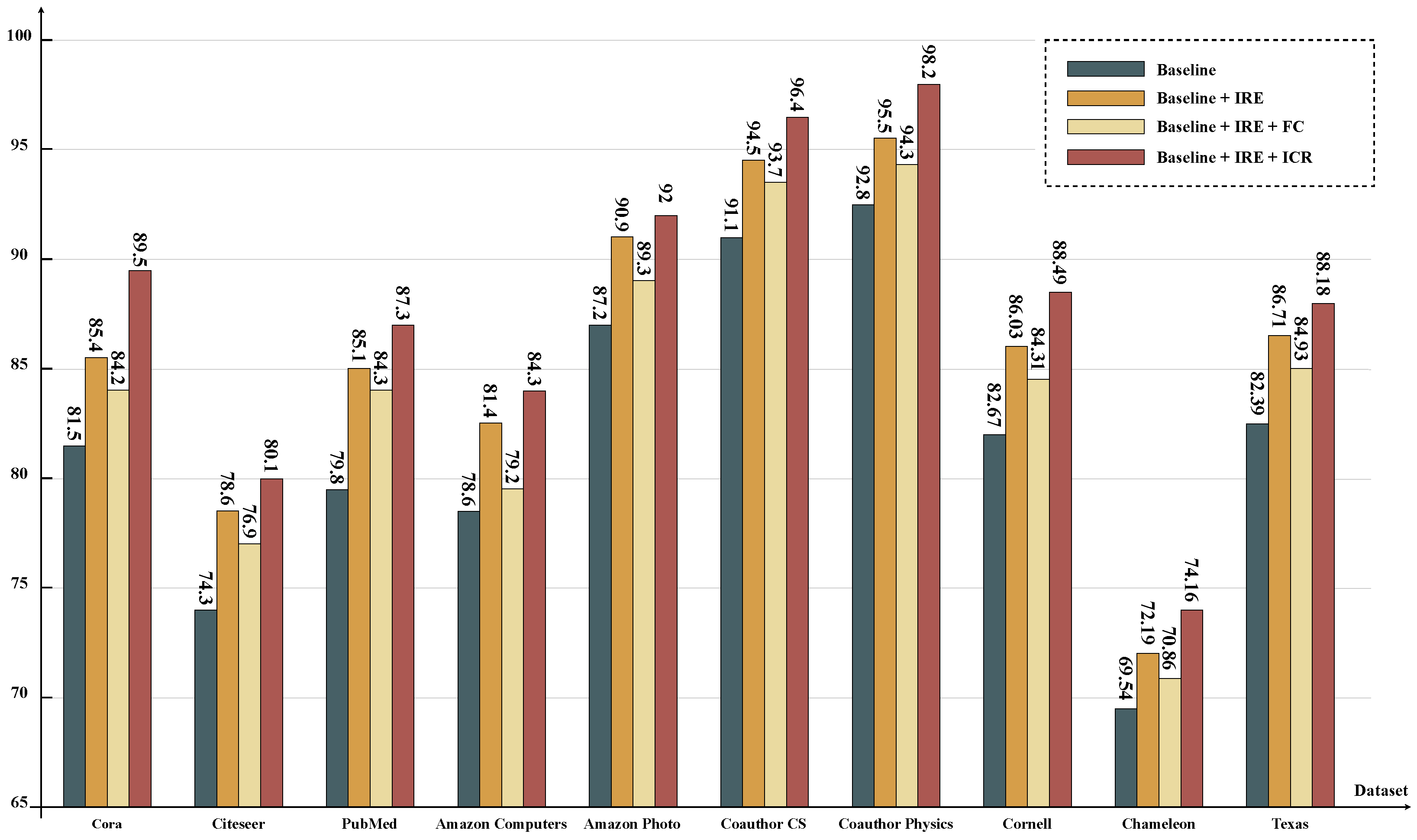
In this section, we describe a series of experiments on the above ten datasets in which we assessed the effectiveness of the IRE and ICR modules in the node classification tasks. As depicted in Figure 3, the experimental results provide valuable insights into the significance of incorporating IRE and ICR modules in the classification process.

Figure 3.
The evaluation results of models with different branch settings are compared on ten datasets, using a simplified version of GCN as the baseline.
Taking the Cora dataset as an example, the baseline achieved an initial accuracy of 81.5%. However, upon integrating the IRE, the accuracy significantly improved by 3.9% to reach 85.4%. This enhancement can be attributed to the IRE’s ability to effectively analyze the structural differences between nodes, advancing the accuracy. Interestingly, the addition of an extra FC slightly decreased the accuracy by 0.8%, emphasizing the importance of proper module integration. However, when the ICR was incorporated, which further considered the impact of node attributes, the accuracy reached its highest value at 87.3%. This highlights the critical role of the ICR in capturing contextual information and boosting the overall model performance. Similar trends were observed across the remaining nine datasets, showcasing the consistent impact of the IRE and ICR in enhancing the model’s ability to analyze complex structures and dependencies. By comprehensively understanding the information propagation mechanism within the graph, the combined IRE and ICR effectively improved the task performance.
The outcomes underscore the importance of integrating both the IRE and ICR in tasks related to node classification for enhanced accuracy and improved interpretability. By introducing the IRE, the model becomes adept at discerning the structural variances, offering clearer insights into how the nodes relate structurally. Incorporating the ICR allows the model to recognize the impact of the node characteristics, providing a more intuitive understanding of the node attributes and their influence on classification. These insights stress the value of considering both the relationships between nodes and the internal features of nodes in graph representation learning. This multifaceted approach bolsters performance while enriching the interpretability of the model’s decisions, setting the stage for crafting efficient and interpretable graph neural network models for diverse graph-centric applications.
5. Conclusions
This paper introduces a novel GNN model, which we call the DAG, which is primarily designed for node classification tasks. The proposed approach aims to enhance task performance by exploring the message-passing mechanisms between nodes at both internode and intra-node levels. The DAG prioritizes the adjacent nodes and node attribute features on the graph structure, significantly improving the performance of node classification tasks on ten graph datasets. It introduces three new features: (i) category-oriented feature attention coefficients to explore node attributes, (ii) a graph feature pooling filter to investigate representative attributes, and (iii) priority filtering of cross-category node features on the mask matrix. We believe that the potential of GNN for other practical applications is worth further research and exploration and serves as a source of inspiration for future studies in this field. Our current method, due to the adoption of a dual attention mechanism, has shown performance improvement. However, in terms of the overall model architecture, computational complexity remains a challenge. Therefore, in the future, we aim to refine our algorithm and focus on overcoming this technical obstacle to achieve a dual breakthrough in performance and computational efficiency, in order to better adapt to various tasks.
Author Contributions
Conceptualization, S.L. and L.H.; methodology, S.L.; software, J.H.; validation, S.L., J.H. and L.H.; formal analysis, B.L.; investigation, S.L.; resources and data curation, J.H.; writing—original draft preparation, S.L.; writing—review and editing, J.H. and L.H.; visualization, B.L.; supervision and project administration, L.H.; All authors have read and agreed to the published version of the manuscript.
Funding
This research received no external funding.
Institutional Review Board Statement
Not applicable.
Informed Consent Statement
Not applicable.
Data Availability Statement
The datasets mentioned in this paper are accessible via the cited publications.
Conflicts of Interest
The authors declare no conflict of interest.
Abbreviations
The following abbreviations are used in this manuscript:
| DAG | Dual Attention Graph Representation Learning |
| GNNs | Graph Neural Networks |
| GCN | Graph Convolutional Network |
| DCNN | Diffusion Convolutional Neural Networks |
| GAT | Graph Attention Networks |
| GIN | Graph Isomorphism Networks |
| GTN | Graph Transformer Networks |
| GraphCL | Graph Contrastive Learning |
| GAE | Graph Autoencoders |
| ICR | Intra-node Contextual Reasoning |
| IRE | Internode Representation Encoding |
| OFM | Origin Feature Matrix |
| UFM | Updated Feature Matrix |
| GAM | Graph Adjacency Matrix |
| UNM | Updated Node Matrix |
| FAM | Fused Attention Matrix |
| FC | Feature Compression |
| FD | Feature Diffusion |
| ELUs | Exponential Linear Units |
| GD | Graph Decipher |
| GSG | GraphSAGE |
References
- Fan, W.; Ma, Y.; Li, Q.; He, Y.; Zhao, E.; Tang, J.; Yin, D. Graph neural networks for social recommendation. In Proceedings of the World Wide Web Conference, San Francisco, CA, USA, 13–17 May 2019; pp. 417–426. [Google Scholar]
- Wang, H.; Zhang, F.; Zhang, M.; Leskovec, J.; Zhao, M.; Li, W.; Wang, Z. Knowledge-aware graph neural networks with label smoothness regularization for recommender systems. In Proceedings of the 25th ACM SIGKDD International Conference on Knowledge Discovery & Data Mining, Anchorage, AK, USA, 4–8 August 2019; pp. 968–977. [Google Scholar]
- Kumar, I.; Hu, Y.; Zhang, Y. Eflec: Efficient feature-leakage correction in gnn based recommendation systems. In Proceedings of the 45th International ACM SIGIR Conference on Research and Development in Information Retrieval, Madrid, Spain, 11–15 July 2022; pp. 1885–1889. [Google Scholar]
- Huang, T.; Dong, Y.; Ding, M.; Yang, Z.; Feng, W.; Wang, X.; Tang, J. Mixgcf: An improved training method for graph neural network-based recommender systems. In Proceedings of the 27th ACM SIGKDD Conference on Knowledge Discovery & Data Mining, Singapore, 14–18 August 2021; pp. 665–674. [Google Scholar]
- Nguyen, T.; Le, H.; Quinn, T.P.; Nguyen, T.; Le, T.D.; Venkatesh, S. GraphDTA: Predicting drug–target binding affinity with graph neural networks. Bioinformatics 2021, 37, 1140–1147. [Google Scholar] [CrossRef]
- Zhang, X.M.; Liang, L.; Liu, L.; Tang, M.J. Graph neural networks and their current applications in bioinformatics. Front. Genet. 2021, 12, 690049. [Google Scholar]
- Pfeifer, B.; Saranti, A.; Holzinger, A. GNN-SubNet: Disease subnetwork detection with explainable graph neural networks. Bioinformatics 2022, 38, ii120–ii126. [Google Scholar] [CrossRef]
- Zhou, F.; Yang, Q.; Zhong, T.; Chen, D.; Zhang, N. Variational graph neural networks for road traffic prediction in intelligent transportation systems. IEEE Trans. Ind. Inform. 2020, 17, 2802–2812. [Google Scholar]
- Xie, Y.; Xiong, Y.; Zhu, Y. SAST-GNN: A self-attention based spatio-temporal graph neural network for traffic prediction. In Proceedings of the Database Systems for Advanced Applications: 25th International Conference, DASFAA 2020, Jeju, Republic of Korea, 24–27 September 2020; Proceedings, Part I 25. Springer: Berlin/Heidelberg, Germany, 2020; pp. 707–714. [Google Scholar]
- Hu, X.; Zhao, C.; Wang, G. A traffic light dynamic control algorithm with deep reinforcement learning based on GNN prediction. arXiv 2020, arXiv:2009.14627. [Google Scholar]
- Liu, B.; Wu, L. Graph Neural Networks in Natural Language Processing. In Graph Neural Networks: Foundations, Frontiers, and Applications; Springer: Berlin/Heidelberg, Germany, 2022; pp. 463–481. [Google Scholar]
- Vashishth, S.; Yadati, N.; Talukdar, P. Graph-based deep learning in natural language processing. In Proceedings of the 7th ACM IKDD CoDS and 25th COMAD; ACM: New York, NY, USA, 2020; pp. 371–372. [Google Scholar]
- Jiang, D.; Wu, Z.; Hsieh, C.Y.; Chen, G.; Liao, B.; Wang, Z.; Shen, C.; Cao, D.; Wu, J.; Hou, T. Could graph neural networks learn better molecular representation for drug discovery? A comparison study of descriptor-based and graph-based models. J. Cheminformatics 2021, 13, 1–23. [Google Scholar]
- Li, X.S.; Liu, X.; Lu, L.; Hua, X.S.; Chi, Y.; Xia, K. Multiphysical graph neural network (MP-GNN) for COVID-19 drug design. Briefings Bioinform. 2022, 23, bbac231. [Google Scholar] [CrossRef]
- Han, K.; Lakshminarayanan, B.; Liu, J. Reliable graph neural networks for drug discovery under distributional shift. arXiv 2021, arXiv:2111.12951. [Google Scholar]
- Liu, Z.; Dou, Y.; Yu, P.S.; Deng, Y.; Peng, H. Alleviating the inconsistency problem of applying graph neural network to fraud detection. In Proceedings of the 43rd International ACM SIGIR Conference on Research and Development in Information Retrieval, Virtual Event, China, 25–30 July 2020; pp. 1569–1572. [Google Scholar]
- Deng, A.; Hooi, B. Graph neural network-based anomaly detection in multivariate time series. Proc. Aaai Conf. Artif. Intell. 2021, 35, 4027–4035. [Google Scholar]
- Liu, Y.; Ao, X.; Qin, Z.; Chi, J.; Feng, J.; Yang, H.; He, Q. Pick and choose: A GNN-based imbalanced learning approach for fraud detection. In Proceedings of the Web Conference 2021, Ljubljana, Slovenia, 12–16 April 2021; pp. 3168–3177. [Google Scholar]
- Tolstaya, E.; Gama, F.; Paulos, J.; Pappas, G.; Kumar, V.; Ribeiro, A. Learning decentralized controllers for robot swarms with graph neural networks. Proc. Conf. Robot. Learn. 2020, 100, 671–682. [Google Scholar]
- Li, Q.; Lin, W.; Liu, Z.; Prorok, A. Message-aware graph attention networks for large-scale multi-robot path planning. IEEE Robot. Autom. Lett. 2021, 6, 5533–5540. [Google Scholar] [CrossRef]
- Li, Q.; Gama, F.; Ribeiro, A.; Prorok, A. Graph neural networks for decentralized multi-robot path planning. In Proceedings of the 2020 IEEE/RSJ International Conference on Intelligent Robots and Systems (IROS), Las Vegas, NV, USA, 25–29 October 2020; pp. 11785–11792. [Google Scholar]
- Min, S.; Gao, Z.; Peng, J.; Wang, L.; Qin, K.; Fang, B. STGSN—A Spatial–Temporal Graph Neural Network framework for time-evolving social networks. Knowl.-Based Syst. 2021, 214, 106746. [Google Scholar] [CrossRef]
- Guo, Z.; Wang, H. A deep graph neural network-based mechanism for social recommendations. IEEE Trans. Ind. Inform. 2020, 17, 2776–2783. [Google Scholar] [CrossRef]
- Tong, Z.; Liang, Y.; Sun, C.; Rosenblum, D.S.; Lim, A. Directed graph convolutional network. arXiv 2020, arXiv:2004.13970. [Google Scholar]
- Huang, Z.; Lin, Z.; Gong, Z.; Chen, Y.; Tang, Y. A two-phase knowledge distillation model for graph convolutional network-based recommendation. Int. J. Intell. Syst. 2022, 37, 5902–5923. [Google Scholar] [CrossRef]
- Ruiz, L.; Gama, F.; Ribeiro, A. Gated graph recurrent neural networks. IEEE Trans. Signal Process. 2020, 68, 6303–6318. [Google Scholar] [CrossRef]
- Chen, X.; Zhang, F.; Zhou, F.; Bonsangue, M. Multi-scale graph capsule with influence attention for information cascades prediction. Int. J. Intell. Syst. 2022, 37, 2584–2611. [Google Scholar] [CrossRef]
- Kipf, T.N.; Welling, M. Semi-supervised classification with graph convolutional networks. arXiv 2016, arXiv:1609.02907. [Google Scholar]
- Hamilton, W.L.; Ying, R.; Leskovec, J. Inductive representation learning on large graphs. In Proceedings of the 31st International Conference on Neural Information Processing Systems, Long Beach, CA, USA, 4–9 December 2017; pp. 1025–1035. [Google Scholar]
- Defferrard, M.; Bresson, X.; Vandergheynst, P. Convolutional neural networks on graphs with fast localized spectral filtering. Adv. Neural Inf. Process. Syst. 2016, 29. [Google Scholar]
- Atwood, J.; Towsley, D. Diffusion-convolutional neural networks. Adv. Neural Inf. Process. Syst. 2016, 29. [Google Scholar]
- Velickovic, P.; Cucurull, G.; Casanova, A.; Romero, A.; Lio, P.; Bengio, Y. Graph Attention Networks. Stat 2018, 1050, 4. [Google Scholar]
- Xu, K.; Hu, W.; Leskovec, J.; Jegelka, S. How powerful are graph neural networks? arXiv 2018, arXiv:1810.00826. [Google Scholar]
- Yun, S.; Jeong, M.; Kim, R.; Kang, J.; Kim, H.J. Graph transformer networks. Adv. Neural Inf. Process. Syst. 2019, 32. [Google Scholar]
- Zeng, H.; Zhou, H.; Srivastava, A.; Kannan, R.; Prasanna, V. Graphsaint: Graph sampling based inductive learning method. arXiv 2019, arXiv:1907.04931. [Google Scholar]
- Donnat, C.; Zitnik, M.; Hallac, D.; Leskovec, J. Learning structural node embeddings via diffusion wavelets. In Proceedings of the 24th ACM SIGKDD International Conference on Knowledge Discovery & Data Mining, London, UK, 19–23 August 2018; pp. 1320–1329. [Google Scholar]
- You, Y.; Chen, T.; Sui, Y.; Chen, T.; Wang, Z.; Shen, Y. Graph contrastive learning with augmentations. Adv. Neural Inf. Process. Syst. 2020, 33, 5812–5823. [Google Scholar]
- Kipf, T.N.; Welling, M. Variational graph auto-encoders. arXiv 2016, arXiv:1611.07308. [Google Scholar]
- Zhang, J.; Shi, X.; Xie, J.; Ma, H.; King, I.; Yeung, D.Y. Gaan: Gated attention networks for learning on large and spatiotemporal graphs. arXiv 2018, arXiv:1803.07294. [Google Scholar]
- Pang, Y.; Zhang, X.; Li, J.; Zhang, H.; Liu, W. Graph Decipher: A transparent dual-attention graph neural network to understand the message-passing mechanism for the node classification. Int. J. Intell. Syst. 2022, 37, 8747–8769. [Google Scholar] [CrossRef]
- Zhu, J.; Yan, Y.; Zhao, L.; Heimann, M.; Akoglu, L.; Koutra, D. Beyond homophily in graph neural networks: Current limitations and effective designs. Adv. Neural Inf. Process. Syst. 2020, 33, 7793–7804. [Google Scholar]
- Du, L.; Shi, X.; Fu, Q.; Ma, X.; Liu, H.; Han, S.; Zhang, D. Gbk-gnn: Gated bi-kernel graph neural networks for modeling both homophily and heterophily. In Proceedings of the ACM Web Conference 2022, Lyon, France, 25–29 April 2022; pp. 1550–1558. [Google Scholar]
- Sen, P.; Namata, G.; Bilgic, M.; Getoor, L.; Galligher, B.; Eliassi-Rad, T. Collective classification in network data. AI Mag. 2008, 29, 93. [Google Scholar] [CrossRef]
- Namata, G.; London, B.; Getoor, L.; Huang, B.; EDU, U. Query-driven active surveying for collective classification. In Proceedings of the 10th International Workshop on Mining and Learning with Graphs, Brussels, Belgium, 10–12 December 2012; Volume 8. [Google Scholar]
- Rozemberczki, B.; Allen, C.; Sarkar, R. Multi-scale attributed node embedding. J. Complex Netw. 2021, 9, 1–22. [Google Scholar] [CrossRef]
- Shchur, O.; Mumme, M.; Bojchevski, A.; Günnemann, S. Pitfalls of graph neural network evaluation. arXi 2018, arXiv:1811.05868. [Google Scholar]
- McAuley, J.; Targett, C.; Shi, Q.; Van Den Hengel, A. Image-based recommendations on styles and substitutes. In Proceedings of the 38th International ACM SIGIR Conference on Research and Development in Information Retrieval, Santiago, Chile, 9–13 August 2015; pp. 43–52. [Google Scholar]
- Glorot, X.; Bengio, Y. Understanding the difficulty of training deep feedforward neural networks. In Proceedings of the Thirteenth International Conference on Artificial Intelligence and Statistics, JMLR Workshop and Conference Proceedings, Sardinia, Italy, 13–15 May 2010; pp. 249–256. [Google Scholar]
- Clevert, D.A.; Unterthiner, T.; Hochreiter, S. Fast and accurate deep network learning by exponential linear units (elus). arXiv 2015, arXiv:1511.07289. [Google Scholar]
- Ren, Y.; Zhao, P.; Sheng, Y.; Yao, D.; Xu, Z. Robust softmax regression for multi-class classification with self-paced learning. In Proceedings of the 26th International Joint Conference on Artificial Intelligence, Melbourne, Australia, 19–25 August 2017; pp. 2641–2647. [Google Scholar]
- Srivastava, N.; Hinton, G.; Krizhevsky, A.; Sutskever, I.; Salakhutdinov, R. Dropout: A simple way to prevent neural networks from overfitting. J. Mach. Learn. Res. 2014, 15, 1929–1958. [Google Scholar]
- Haonan, L.; Huang, S.H.; Ye, T.; Xiuyan, G. Graph star net for generalized multi-task learning. arXiv 2019, arXiv:1906.12330. [Google Scholar]
- Gao, Y.; Yang, H.; Zhang, P.; Zhou, C.; Hu, Y. Graphnas: Graph neural architecture search with reinforcement learning. arXiv 2019, arXiv:1904.09981. [Google Scholar]
- Zhang, J. Get rid of suspended animation problem: Deep diffusive neural network on graph semi-supervised classification. arXiv 2020, arXiv:2001.07922. [Google Scholar]
- Rychalska, B.; Bąbel, P.; Gołuchowski, K.; Michałowski, A.; Dąbrowski, J.; Biecek, P. Cleora: A simple, strong and scalable graph embedding scheme. In Proceedings of the International Conference on Neural Information Processing, Bali, Indonesia, 8–12 December 2021; pp. 338–352. [Google Scholar]
- Luo, Y.; Luo, G.; Yan, K.; Chen, A. Inferring from References with Differences for Semi-Supervised Node Classification on Graphs. Mathematics 2022, 10, 1262. [Google Scholar] [CrossRef]
- Pei, H.; Wei, B.; Chang, K.C.C.; Lei, Y.; Yang, B. Geom-gcn: Geometric graph convolutional networks. arXiv 2020, arXiv:2002.05287. [Google Scholar]
- Topping, J.; Di Giovanni, F.; Chamberlain, B.P.; Dong, X.; Bronstein, M.M. Understanding over-squashing and bottlenecks on graphs via curvature. arXiv 2021, arXiv:2111.14522. [Google Scholar]
- Zhang, F.; Bu, T.M. CN-Motifs Perceptive Graph Neural Networks. IEEE Access 2021, 9, 151285–151293. [Google Scholar] [CrossRef]
- Yan, Y.; Hashemi, M.; Swersky, K.; Yang, Y.; Koutra, D. Two sides of the same coin: Heterophily and oversmoothing in graph convolutional neural networks. arXiv 2021, arXiv:2102.06462. [Google Scholar]
- Kulatilleke, G.K.; Portmann, M.; Ko, R.; Chandra, S.S. FDGATII: Fast Dynamic Graph Attention with Initial Residual and Identity Mapping. arXiv 2021, arXiv:2110.11464. [Google Scholar]
- Li, X.; Zhu, R.; Cheng, Y.; Shan, C.; Luo, S.; Li, D.; Qian, W. Finding Global Homophily in Graph Neural Networks When Meeting Heterophily. arXiv 2022, arXiv:2205.07308. [Google Scholar]
- Monti, F.; Boscaini, D.; Masci, J.; Rodola, E.; Svoboda, J.; Bronstein, M.M. Geometric deep learning on graphs and manifolds using mixture model cnns. In Proceedings of the IEEE Conference on Computer Vision and Pattern Recognition, Honolulu, HI, USA, 21–26 July 2017; pp. 5115–5124. [Google Scholar]
Disclaimer/Publisher’s Note: The statements, opinions and data contained in all publications are solely those of the individual author(s) and contributor(s) and not of MDPI and/or the editor(s). MDPI and/or the editor(s) disclaim responsibility for any injury to people or property resulting from any ideas, methods, instructions or products referred to in the content. |
© 2023 by the authors. Licensee MDPI, Basel, Switzerland. This article is an open access article distributed under the terms and conditions of the Creative Commons Attribution (CC BY) license (https://creativecommons.org/licenses/by/4.0/).