Abstract
We are devoted, in this paper, to the study of the pre-assigned-time drive-response synchronization problem for a class of Takagi–Sugeno fuzzy logic-based stochastic bidirectional associative memory neural networks, driven by Brownian motion, with continuous-time delay and (finitely and infinitely) distributed time delay. To achieve the drive-response synchronization between the neural network systems, concerned in this paper, and the corresponding response neural network systems (identical to our concerned neural network systems), we bring forward, based on the structural properties, a class of control strategies. By meticulously coining an elaborate Lyapunov–Krasovskii functional, we prove a criterion guaranteeing the desired pre-assigned-time drive-response synchronizability: For any given positive time instant, some of our designed controls make sure that our concerned neural network systems and the corresponding response neural network systems achieve synchronization, with the settling times not exceeding the pre-assigned positive time instant. In addition, we equip our theoretical studies with a numerical example, to illustrate that the synchronization controls designed in this paper are indeed effective. Our concerned neural network systems incorporate several types of time delays simultaneously, in particular, they have a continuous-time delay in their leakage terms, are based on Takagi–Sugeno fuzzy logic, and can be synchronized before any pre-given finite-time instant by the suggested control; therefore, our theoretical results in this paper have wide potential applications in the real world. The conservatism is reduced by introducing parameters in our designed Lyapunov–Krasovskii functional and synchronization control.
Keywords:
bidirectional associative memory neural networks; pre-assigned-time synchronization; Takagi–Sugeno fuzzy logic; time delays; Lyapunov–Krasovskii functional MSC:
93E15; 28E10; 34K20; 34K37; 34K50; 60H10
1. Introduction
In recent years, it was found that neural networks have been widely used in many theoretical and/or application fields; see [1,2,3] and the vast references cited therein. For example, experts and engineers have already utilized suitable neural networks in vast fields such as optimization theory and the related field applications, associative memories, signal processing, and machine learning. As a result, it is extremely interesting and important to invent neural networks having new structural properties to satisfy specific needs and desires. For instance, in the 1980s, Kosko came up with a class of neural networks, nowadays known as bidirectional associative memory neural networks (BAMNNs), to generalize a single-layer auto-associative Hebbian correlator to two-layer pattern-matched hetero-associative circuits; see References [3,4,5,6]. On the other hand, it seems that people are even more interested in quantitatively studying the structural properties of neural networks and in designing the control, based on the obtained structural properties, to improve the properties of neural networks; the related meaningful results can be seen in [1,2,5,7,8,9,10,11,12,13,14,15,16], to name just a few of the vast references.
As a typical phenomenon, chaos occurs frequently in complicated nonlinear dynamical systems; see References [3,6,17]. For example, in Reference [17], a nonlinear financial dynamical system was shown, via a numerical approach, to be chaotic. Chaos in the systems could lead to the high sensitivity of trajectories in their initial states. This brings enormous difficulty in applying systems. Therefore, control strategies (synchronization control, for example) should be designed to reduce or even remove the chaos in the systems. For instance, various synchronization problems associated with neural networks have been studied extensively and intensively in recent years; see References [6,7,9,18].
In this paper, we are interested in the synchronization problem for BAMNNs. As with other neural networks, BAMNNs are of wide applicability, for example, they have been frequently exploited in classification, associative memory, signal processing, image processing, parallel computation, combinatorial optimization, and pattern recognition; see References [1,2,4,19]. BAMNNs have their neurons grouped into two layers (the U-layer and the V-layer, as shall be marked in this paper). The neurons of a BAMNN in one layer are fully interconnected to the neurons in the other layer, while there is no interconnection between any two pair of neurons in the same layer; in BAMNNs, the information flows propagate forward and backward between the two layers. Thanks to such a special structure, experts and engineers can realize in BAMNNs a bidirectional associative search for stored bipolar vector pairs; see References [3,4] and some references cited therein for a more detailed explanation on the importance of BAMNNs.
In real-world applications, the switching speed of amplifiers in the electronic implementation of analog neural networks is finite. This leads to the occurrence of a time delay in the communication and response of neurons. And therefore it seems to be more realistic to study the neural networks with time delays. Zhu and Cao [1], Wang and Zhu [2], and Samidurai, Senthilraj et al. [7] studied BAMNNs with various time delays and obtained a criterion guaranteeing the stability of the equilibrium of their concerned BAMNNs. Yuan, Luo et al. [18] investigated a class of time-delayed memristor-based BAMNNs and applied their obtained theoretical results into the field of image hiding. Time delays would cause difficulties in treating problems related to BAMNNs. In recent years, experts have developed many methods to overcome these difficulties; see [9,18,20,21,22,23,24] and the vast references cited therein. For example, Lin and Zhang [20] established several asymptotic synchronization criteria for a class of BAM neural networks with time delays via integrating inequality techniques, Yang, Chen et al. [21] proved their claimed synchronization results concerning BAMNN via convex analysis, and Yang and Zhang [22] applied the quadratic analysis approach to treat a class of delayed BAMNNs.
The realistic neural networks contain unavoidable uncertainty, due to the transmission of information through neurons. It is well-known that fuzzy logic could play an important role in dealing with uncertainty; see References [5,6,25,26]. Wang, Zhao et al. [6] designed, for a class of fuzzy BAMNNs, some intermittent quantized control, and they provided an interesting criterion ensuring that the controlled BAMNNs achieve finite-time drive-response synchronization. Zhou, Zhang et al. [26] considered the finite-time synchronization problem for fuzzy delayed neutral-type inertial BAM neural networks and obtained some novel criteria by applying integral inequality techniques and the figure analysis approach.
Actually, stochastic BAMNNs have also been widely used in many areas and therefore have aroused a large number of experts’ interest in studying their dynamics from both mathematical and engineering viewpoints. The synaptic transmission in nervous systems can be considered as a noisy process brought on by random fluctuations from the release of neurotransmitters or other probabilistic factors; this would cause some uncertainty which can not be modeled by fuzzy logic but can be modeled by a special stochastic process, such as general martingales, Lévy processes, Markovian chains (time homogeneous or time inhomogeneous), Brownian motions (Wiener processes), and so on; see References [6,27,28] and the vast references cited therein. For example, the BAMNN concerned in Reference [6] is subject to a Markovian chain. As with fuzzy uncertainty, random (or stochastic) uncertainty causes difficulties in deriving synchronization criteria for BAMNNs.
After reviewing References [1,2,3,4,5,6,7,8,9,10,11,17,18,19,20,21,22,23,24,26,27,28,29,30,31,32,33], we are tempted to further investigate BAMNNs for their synchronizability. In the literature, quite a few interesting results were obtained recently in this direction. For example, the finite-time synchronization problems for BAMNNs were treated systematically in References [34,35], the fixed-time synchronization problems associated with BAMNNs were investigated extensively in [36,37] and the references therein, the pre-assigned-time synchronization problems for BAMNNs were also considered in References [38,39,40,41,42,43,44], and some interesting results related to the synchronizability of BAMNNs were presented in References [45,46,47,48,49]. Chen and Zhang [34] as well as Yang and Zhang [35] obtained some finite-time synchronization results for time-delayed BAMNNs via different approaches. As with finite-time synchronizability, fixed-time synchronizability (the synchronization can be realized within a fixed-time instant) seems to have relatively wide applicability but brings on more challenges. Wang, Zhang et al. [36] considered the fixed-time synchronization problem for complex-valued BAMNNs with time-varying delays via (adaptive) pinning control. Duan and Li [37] studied a class of fuzzy neutral-type memristor-based inertial BAMNNs with proportional delays for their fixed-time synchronizability. As mentioned several times above, we consider BAMNNs for their pre-assigned-time synchronizability (the synchronization can be realized within any specified time instant in advance) in this paper. Let us mention here several related results in the literature. Chen, Xiong et al. [44] and Liu, Zhao et al. [43] obtained pre-assigned synchronization results for complex-valued BAMNNs via different approaches. Liu, Zhao et al. [42] applied the pre-assigned synchronization results of complex-valued BAMNNs to image protection. Wang, Zhao et al. [38], Mahemuti and Abdurahman [39], Abdurahman, Abudusaimaiti et al. [40], as well as You, Abdurahman et al. [41] came up with various methods to treat stochastic BAMNNs for their pre-assigned-time synchronizability.
By reviewing the aforementioned references, we conclude that it is interesting to design a pre-assigned-time synchronization control strategy for Takagi–Sugeno logic-based stochastic BAMNNs with continuous-time delay in leakage terms and with continuous-time delay and (finitely/infinitely) distributed-time delay in transmission terms, and it is interesting to provide a criterion ensuring that our concerned BAMNNs (viewed as the drive network systems) and the response BAMNNs, with our proposed control implemented, achieve synchronization within the pre-defined time.
Notational Conventions. We write for the totality of real numbers, and , for the closed interval , the closed interval , respectively. denotes the right upper Dini derivative of the given function f with respect to the independent variable t. denotes the usual Lebesgue measure space. We designate by (or ) a complete filtered probability space, in which the filtration is assumed to satisfy the usual conditions; in other words, the -algebra contains all -null sets in the -algebra , and is right-continuous in the sense that
“ almost surely” is abbreviated as -a.s.; denotes the mathematical expectation of X, where X is an arbitrarily given random variable on ; denotes the product measure space of and ; and , an -adapted stochastic process, denotes a one-dimensional standard Brownian motion (Wiener process) defined on the probability space . denotes the cardinality of a set A.
The remainder of this paper is organized as follows. In Section 2, we formulate our concerned synchronization problem for BAMNNs and present some preliminaries necessary for our later description. In Section 3, we state our main result in this paper and provide in detail the proof. In Section 4, we validate, numerically and visually, our theoretical results via coming up with specific example BAMNNs which display the chaos phenomenon and verifying that the example BAMNNs and the corresponding response BAMNNs with our proposed control implemented achieve synchronization within the pre-assigned time. In Section 5, we provide several concluding remarks.
2. Problem Formulation and Preliminaries
In this section, our principal aim is to state our problem and the main mathematical tools to be used to treat our problem. We shall explicitly present our model BAMNNs, explain in some detail the structure of our concerned model BAMNNs, formulate clearly our problem considered in this paper, and prepare some key ingredients to be used in our later treatment of the main problem in this paper.
Let p and r be given positive integers and a fuzzy set, more precisely, a function mapping into , , . In this paper, we assume that our concerned BAMNNs obey the Takagi–Sugeno IF–THEN rule. By the “BAMNNs obey the Takagi–Sugeno IF–THEN rule”, we mean IF the premise variable is , , THEN the dynamics of our concerned BAMNNs are governed by the following coupled system of forward stochastic differential equations
supplemented by the initial condition
in which the stochastic processes , , , and , required to be -adapted, are given in detail by
where is the filtration, required to satisfy the usual conditions (see the paragraph of notational conventions in Section 1 for the detailed explanation), of a complete filtered probability space . The stochastic process denotes, throughout this paper, a one-dimensional standard Brownian motion (Wiener process) defined on the probability space . Let us spare here some more lines to explain our model BAMNNs (1)-(2)-(3). ℶ and ℷ are two given sets containing finitely many elements (let us remind that and denote the cardinality of ℶ and ℷ, respectively). The constants and are the amplification coefficients of the neurons themselves; and are activation functions; the real constants and are connection coefficients; the functions and represent (continuous-)time delays in leakage (also known as forgetting) terms; the functions and , and , as well as and represent (continuous-)time delays in transmission terms; the functions and , and , as well as and represent distributed time delays in transmission terms; the functions and are kernels of the infinitely distributed time delays in transmission terms; the stochastic processes and , required to be -adapted, are the state trajectories of our concerned BAMNNs (1)-(2)-(3); the stochastic processes , , , and represent the overall exogenous disturbance; the -adapted stochastic processes and represent the instant exogenous disturbance; the -adapted stochastic processes and represent the exogenous disturbance subject to the continuous-time delay effect; the -adapted stochastic processes and represent the exogenous disturbance subject to the finitely distributed time delay effect; the -adapted stochastic processes and represent the exogenous disturbance subject to the infinitely distributed time delay effect; the -adapted stochastic processes and represent the other exogenous disturbance which can not be described as the aforementioned types of exogenous disturbance; and the initial data (stochastic processes) and , functions mapping into , are -measurable (see Section 1 for the definition of ). In addition, and are -measurable for all , and have their path essentially bounded in , -a.s., where , , , , , .
As usual, to proceed further, we need to defuzzify the Takagi–Sugeno fuzzy BAMNNs (1)-(2)-(3). Let us denote by the grade of membership of the element (viewed as premise variable) and now introduce the following weight functions
in which and , . Aided by (see (4)), we can defuzzify the Takagi–Sugeno BAMNNs (1)-(2)-(3) into
where the initial data stochastic processes and are given, respectively, by
and
the coefficients , , , and , , are given by
the exogenous disturbances and are given, respectively, by
and
Now, we are in a position to introduce the response BAMNNs
where the initial data stochastic processes and are given, respectively, by
and
with the given initial data stochastic processes and being -measurable and being -measurable for all , the exogenous disturbances and are given as in (6) and (7), respectively, and the -adapted stochastic processes and are the control inputs. To study the claimed identical synchronization problem in the pre-assigned time, we need to introduce the error BAMNNs
where the stochastic processes, as in (8), and , are the control inputs, the state trajectories and of the error BAMNNs (11) are given, respectively, by
and
and the functions and are given, respectively, by
and
Throughout this paper, we assume that the activation functions and are Lipschitz continuous and have positive constants as the lower bounds of their difference quotients, that the functions , , , and satisfy some regularity and growth conditions, and that the kernels and are Lebesgue integrable, , , , , ; see Assumptions 1–3 for the details.
Assumption 1.
There exist positive constants , , , and , satisfying the inequality condition and , such that
and
Assumption 2.
The continuous functions , , , and , mapping into itself, satisfy , , , and for all , , , . The functions , , , and are differentiable in and are Lipschitz continuous in , so it holds that , , , and , where the constants , , , and are given, respectively, by
and in addition, it holds that , as well as , in which the constants and are given, respectively, by
Assumption 3.
The kernels and are continuous functions mapping into itself, and they are Lebesgue integrable in every compact subinterval of , , , . Moreover, the kernels and satisfy
For the sake of convenience, we introduce here the constants and by
and
Remark 1.
Suppose that the stochastic processes , , , , , , , , , , , and are all -adapted, , , . Under Assumptions 1–3, for any initial data stochastic processes and , as well as and , functions mapping into , being -measurable, being -measurable for all , being almost surely bounded in , and satisfying
, , , the BAMNNs (1)-(2)-(3), BAMNNs (5)-(6)-(7), BAMNNs (8)-(6)-(7), and error BAMNNs (11) admit a unique state trajectory, respectively.
Definition 1
([11]). The drive BAMNNs (5)-(6)-(7) and the response BAMNNs (8)-(6)-(7) are said to achieve synchronization in a pre-assigned settling time, or to achieve pre-assigned-time synchronization, provided that for any given positive time instant T, there exists a collection of control inputs , , , , such that for any state trajectory , of BAMNNs (5)-(6)-(7) (the drive network systems), and any state trajectory , of BAMNNs (8)-(6)-(7) (the response network systems), with our designed control implemented, it holds always that
where , together with , given by (12), together with (13), denotes the state trajectory of the error BAMNNs (11).
To put it concisely, observing that the functions and are continuous in time t, , , we conclude, by Definition 1, that proving BAMNNs (5)-(6)-(7) and BAMNNs (8)-(6)-(7) achieve drive-response synchronization within the pre-assigned time T boils down to proving for all , , .
Illuminated by References [11,44], we define an important auxiliary function:
in which is the celebrated Euler’s Beta function, which is explicitly given by
and is the so-called incomplete Beta function, which is defined by
Lemma 1
([11]). Let , (), , , and be given. For any decreasing function (mapping of into itself) satisfying
it holds that for all , where is given as in (19).
3. Main Results and Their Proofs
In this section, our main aim is to state our main results in this paper and to provide detailed proofs of our claimed theoretical results. We shall first come up with a class of synchronization control inputs for the response BAMNNs (8)-(6)-(7), construct secondly a suitable Lyapunov–Krasovskii functional along the state trajectories of the error BAMNNs (11), and finally establish, with our cleverly developed Lyapunov–Krasovskii functional as the key ingredient, a criterion ensuring that BAMNNs (5)-(6)-(7) and BAMNNs (8)-(6)-(7), with our designed control implemented, achieve pre-assigned-time synchronization.
To obtain our desired pre-assigned-time synchronization, we put forward, after some basic analysis, the following synchronization control
and
in which the positive constant is fixed arbitrarily small, the positive constants and are yet to be determined, , and the stochastic process is given by
in which the constants , , , , , , , , , , , , , , , and are to be determined suitably, where , , , . Following the basic idea to obtain a pre-assigned-time synchronization criterion, we introduce the auxiliary functional
where is the Lyapunov–Krasovskii functional candidate that is given by
in which , , and are defined, respectively, by
and
Theorem 1.
Suppose that Assumptions 1–3 hold true. Let be given. If there exist some positive constants , , , , , , , , , , , , , , , , , , , , , , , (, , , ), and the constants , , and such that the function given by (24) satisfies the differential inequality (20) in Lemma 1 and it holds that where is defined as in (19) and the constant is given by
with the constants , , and given, in turn, by (29), (30), and (31), respectively, then the drive BAMNNs (5)-(6)-(7) and the response BAMNNs (8)-(6)-(7), with the control (21)-(22) implemented, achieve synchronization within the pre-assigned time .
Proof.
From the analysis conducted in Section 2, we realize that to prove Theorem 1, it boils down to proving a stability criterion for the error BAMNNs (11). To establish the desired stability criterion, we have to analyze in some detail the Lyapunov–Krasovskii functional , defined as in (25), and its mathematical expectation , given by (24). Apply Itô’s differentiation rule to given by (26) to obtain
By some routine calculations, we have
By applying mainly
as well as Leibniz’s integral rule, we have
Mimick steps to obtain (35), to arrive at
Borrowing an idea from the derivation of (37), we have by some routine calculations
Apply Itô’s differentiation rule to given by (25), to find that there exist two -adapted stochastic processes and such that
or equivalently
where the stochastic process is given by
Combine (35) and (37)–(39) to obtain
in which the second “⩽” follows directly from the next inequality
where the stochastic processes and satisfy
with defined as in (23), the constant is given as in (32), and the stochastic process is given as in (25). Thanks to (32) (as well as (23) and (42)), the collection of constants , , , , , , , , , , , , , , , and the collection of constants , influence each other, and both collections, together with the collection of constants, constant , depend on , , , , , , , , , , , and , , , , , , , , .
To facilitate our later presentation, we would like to treat our problems from two different perspectives. We consider first the following situation:
In this case, the state of the error BAMNNs (11) arrives at the null state or, equivalently, our concerned drive BAMNNs (5)-(6)-(7) and response BAMNNs (8)-(6)-(7) are already synchronized. Now, we are in a position to consider the following situation:
By Lebesgue’s dominated convergence theorem, we derive from (43) and (44) that
where the constant is defined as in (33), and the function is defined by (19). To obtain the “⩽” next to the last line of (45), we used the assumption that and the following inequality (can be deduced by Jensen’s inequality):
Recalling (45) and passing to the limit, we have immediately
By Lemma 1, this implies that the proof of Theorem 1 is complete. □
4. Numerical Validation of Our Theoretical Results
In this section, we are devoted to the numerical simulations of the validity of our aforementioned synchronization criterion (see Theorem 1). We assume that the defuzzified network system of our concerned multiplied time-delayed BAM based on the Takagi–Sugeno IF–THEN logic is of the form (5), in which we assume basically throughout this section that , , and . We assume in this example that
and
and, as a consequence, we have
and
We assume that the time delays , , and in the leakage terms of our concerned example BAM are given, respectively, by
In the meantime, we assume that the time delays , , , , , , , , , , , , , , , and in the transmission terms of our concerned example BAM are given, respectively, by
Suppose also in our concerned example BAM that , , , , , and . We assume throughout this section that the kernels , , , , , , , and are defined, respectively, by
For the sake of the convenience of our later numerical simulations, we assume that
We assume that the transmission connection weight coefficients satisfy
We assume that the activation functions , , , , , , , , , , , , , , , , , , , , , , , and are given, respectively, by
in which the functions , , and are, respectively, defined by
and
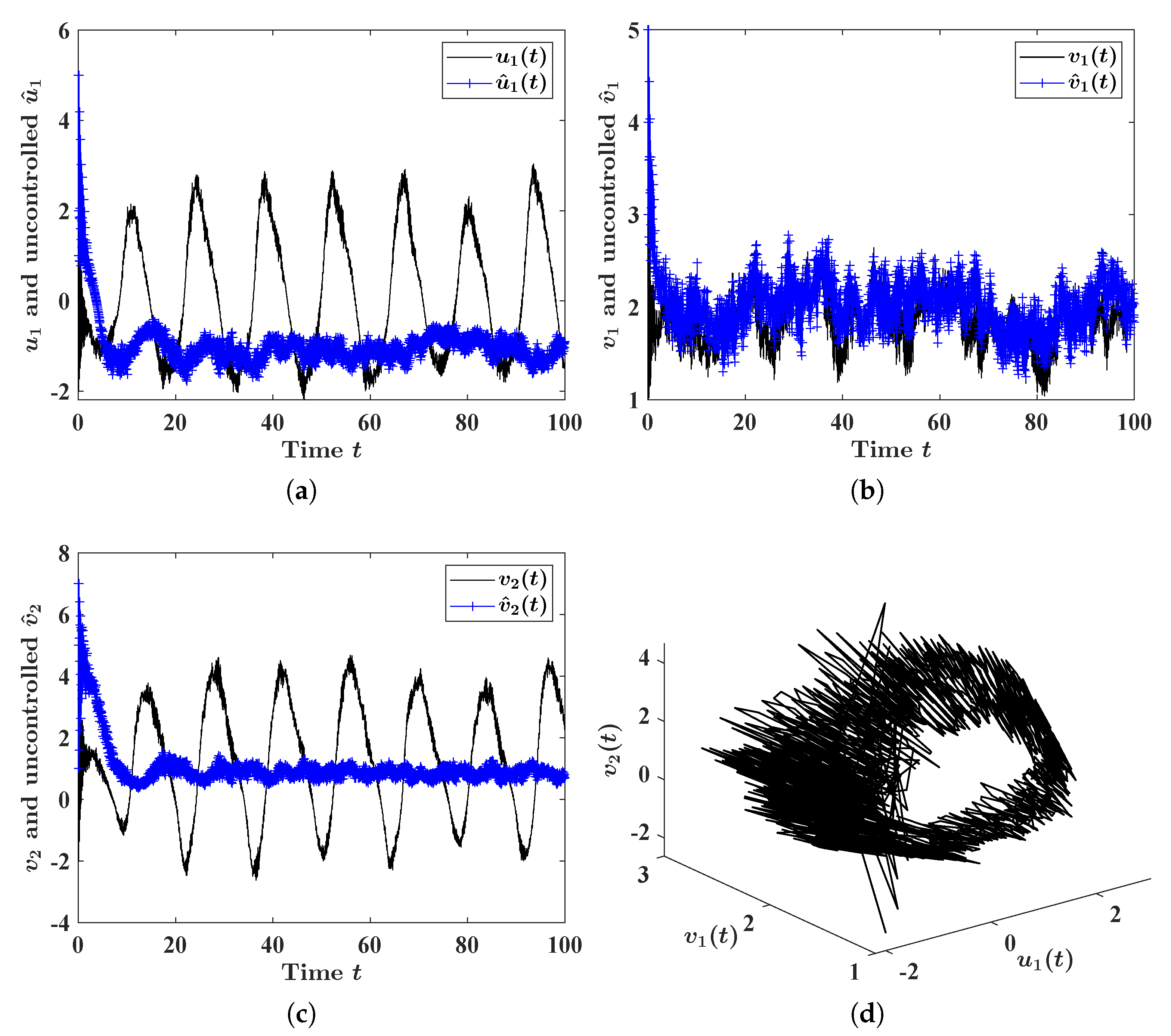
The chaos phenomenon occurs frequently in many complicated nonlinear differential dynamical systems. Chaos could prevent some pairs of different state trajectories of the concerned dynamical system from approaching each other as time escapes to infinity. That is, chaotic dynamical systems do not achieve identical synchronization automatically. And, therefore, experts have been attracted to designing suitable controls to synchronize chaotic dynamical systems; see [6,17] and the vast references mentioned therein.
To “demonstrate” that our proposed synchronization control essentially improves the structural property of the example BAMNN concerned in this section, we first show via MATLAB software that our concerned example BAMNN could be “chaotic”. To this end, we solve first numerically the solution, denoted by throughout this section, to our concerned example BAMNN, of which the initial data are composed of data in two modes, namely, and , where
and
See Figure 1 (including subfigures (a), (b), (c), and (d)) for the detailed description of the graph of the state trajectory , . And, similarly, we solve numerically the solution, denoted by , to the response BAMNN associated with our concerned drive BAMNN, of which the initial data are composed of data in two modes, namely, and , where
and

Figure 1.
Numerical and graphical illustration of the occurrence of chaos phenomenon in the example BAMNN concerned in this section. , , is the state trajectory triple of our concerned example BAMNN with , , and , , -a.s.; see (a–c) for the graph (the solid curves) of the functions , , in the interval . The graph of the parametric curve is visualized in the phase space (state space); see (d). , , is the state trajectory triple of the response BAMNN with no controls implemented, associated with our concerned example BAMNN, with , , and , , -a.s.; see also (a–c) for the graph (the curves composed of “+”) of the functions , , in .
The detailed description of the graph of the state trajectory , , can also be seen in Figure 1 (including subfigures (a), (b), and (c)). To summarize, we “demonstrate”, by Figure 1, in a visual way, that our concerned example BAMNN is “chaotic”, in particular, some of the trajectories are sensitive to their initial states. We next show numerically that our proposed control law (21)-(22) could effectively synchronize our concerned example BAMNN in any pre-assigned time: For any given positive time instant T, our example BAMNN and the corresponding controlled response system achieve synchronization before with ; see Figure 2 and Figure 3 for the details.
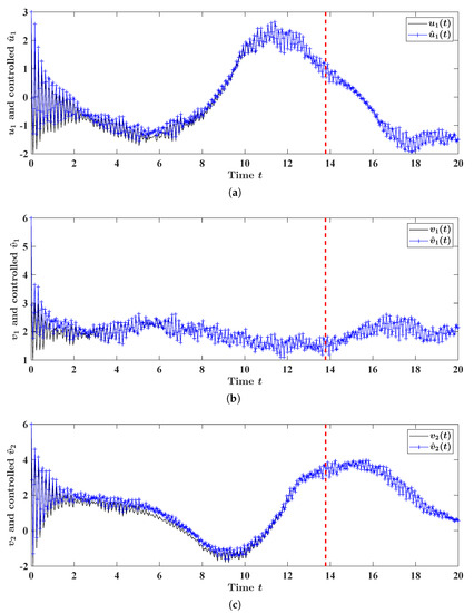
Figure 2.
Numerical and graphical validation of our theoretical synchronization results; see Theorem 1 for the details. As in Figure 1, , (see the solid curves in (a–c)), is the state trajectory triple of our concerned example BAMNN with , , and , , -a.s. , (see the curves composed of “+” in (a–c)), is the state trajectory triple of the controlled response BAMNN associated with our concerned example BAMNN with , , and , , -a.s. The dashed straight vertical line segments are the graphs of .
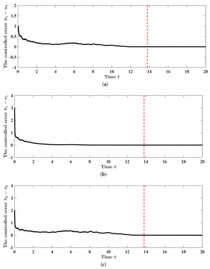
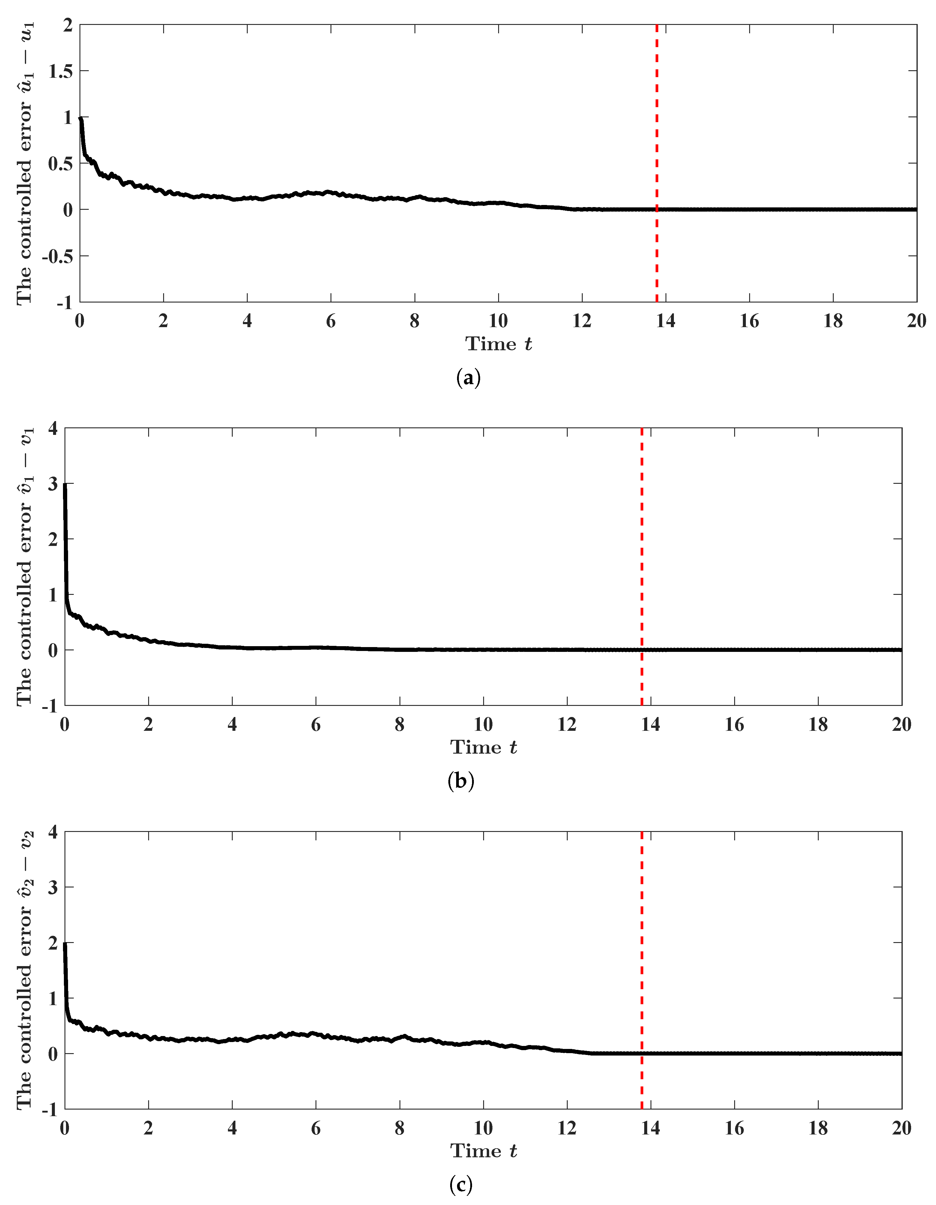
Figure 3.
Numerical and graphical validation of our theoretical synchronization results; see Theorem 1 for the details. As in Figure 1 and Figure 2, , , is the state trajectory triple of the error system, in which , , is the state trajectory triple of our concerned example BAMNN with , , and , , -a.s. , , is the state trajectory triple of the controlled response BAMNN associated with our concerned example BAMNN with , , and , , -a.s. The dashed straight vertical line segments are the graphs of . The graphs of the tracking error , and can be seen in (a–c).
5. Concluding Remarks
In this paper, we studied a class of time-delayed stochastic BAMNNs, namely, BAMNNs (1)-(2)-(3), based on the Takagi–Sugeno IF–THEN logic and driven by a one-dimensional standard Brownian motion (also termed the Wiener process). Our concerned BAMNNs include a continuous-time delay in leakage terms and a continuous-time delay and (finitely as well as infinitely) a time-distributed delay in transmission terms. Our study, in this paper, is inspired considerably by References [1,2,3,4,5,6,7,11,36,37,38,40,43,44], but we are confronted with quite a few new challenges. For example, different from References [1,3,5,7,11,36,38,43,44], we have to apply a technique to overcome the difficulty brought on by the infinitely time-distributed delay in transmission terms of our concerned BAMNNs, or as opposed to References [5,6], we have to find a new clue to cope with the difficulty caused by the Takagi–Sugeno fuzzy logic in the concerned BAMNNs.
In this paper, we designed a class of control for our concerned BAMNNs and provided a criterion to ensure that our concerned BAMNNs and their response BAMNNs, with our designed control implemented, achieve synchronization within the pre-assigned time. In more detail: (i) We followed the common idea utilized to deal with Takagi–Sugeno fuzzy dynamical systems, to defuzzify the Takagi–Sugeno fuzzy BAMNNs (1)-(2)-(3) into BAMNNs (5)-(6)-(7); (ii) we designed, based on the structure of the response BAMNNs (8)-(6)-(7) of BAMNNs (5)-(6)-(7), the synchronization control (21)-(22); (iii) for any pre-specified time instant (T, say), we established a criterion, meticulously constructed the Lyapunov–Krasovskii functional (see (25)), and proved that the BAMNNs (5)-(6)-(7) and the response BAMNNs (8)-(6)-(7), with the control (21)-(22) implemented, achieve synchronization within the pre-assigned time T (see Theorem 1 for the details); and (iv) based on the careful and complicated mathematical derivations in Section 3, we came up with an example which validates our main theoretical results in this paper.
One of the merits of our designed control (21)-(22) is that we only render the control (21)-(22) to be implemented in the drift terms of the response BAMNNs (8)-(6)-(7). Another merit of our designed control (21)-(22) is that a collection of parameters are included so as to reduce the conservatism of the synchronization criterion (see Theorem 1). On the other hand, our designed control (21)-(22) has a disadvantage: The aftereffect in our designed control seems to be strong; see (21)-(22) for the details. To remove or attenuate the aftereffect in synchronization control for BAMNNs (1)-(2)-(3) is one of our primary research directions in the near future. And inspired by the research experience of this paper and the references cited in this paper, we shall work in the direction of improving, in a certain sense, synchronization control for BAMNNs (1)-(2)-(3). For example, we shall try to come up with impulsive control, intermittent control, quantized control, adaptive control, pinning control, sliding mode control, event-triggered control, and so forth, to synchronize BAMNNs (1)-(2)-(3) asymptotically, in finite time, in fixed time, or in pre-assigned time.
As mentioned above, and by observing BAMNNs (1)-(2)-(3) (or, equivalently, BAMNNs (5)-(6)-(7), BAMNNs (8)-(6)-(7), and the BAMNN (11)), it is not difficult to confirm that our concerned model BAMNNs include merely a one-dimensional Brownian motion (Wiener process). By reviewing mathematical derivations throughout this paper, we find that our methods can be adapted to treat the multi-dimensional Brownian motion (Wiener process) case. From both the theoretical and applied viewpoint, it is interesting to consider stochastic Takagi–Sugeno fuzzy BAMNNs, including Markovian jumps, reaction–diffusion terms, and/or proportional time delay. Aided by the experience of this paper, we shall study the synchronization problem for BAMNNs with their dynamics influenced by fuzzy logic, randomness described by Brownian motions, randomness described by Markovian jumps, reaction–diffusion terms, and/or proportional time delay in the near future.
Author Contributions
Conceptualization, C.W. (Chengqiang Wang); Methodology, C.W. (Chengqiang Wang) and Z.L.; Software, X.Z., C.W. (Can Wang) and Z.L.; Validation, C.W. (Can Wang); Formal analysis, C.W. (Chengqiang Wang), X.Z. and Z.L.; Investigation, C.W. (Chengqiang Wang), X.Z., C.W. (Can Wang) and Z.L.; Resources, X.Z., C.W. (Can Wang) and Z.L.; Data curation, X.Z. and C.W. (Can Wang); Writing—original draft, C.W. (Chengqiang Wang); Writing—review & editing, C.W. (Chengqiang Wang); Supervision, C.W. (Chengqiang Wang); Funding acquisition, C.W. (Chengqiang Wang). All authors have read and agreed to the published version of the manuscript.
Funding
Chengqiang Wang is supported by the Startup Foundation for Newly Recruited Employees and Xichu Talents Foundation of Suqian University (#2022XRC033), NSFC (#11701050), and Jiangsu Qin-Lan Project of Fostering Excellent Teaching Team, “University Mathematics Teaching Team”.
Conflicts of Interest
The authors declare that they have no conflicts of interest.
References
- Zhu, Q.; Cao, J. Stability analysis of Markovian jump stochastic BAM neural networks with impulse control and mixed time delays. IEEE Trans. Neural Netw. Learn. Syst. 2012, 23, 467–479. [Google Scholar] [CrossRef]
- Wang, T.; Zhu, Q. Stability analysis of stochastic BAM neural networks with reaction-diffusion, multi-proportional and distributed delays. Phys. A Stat. Mech. Its Appl. 2019, 533, 121935. [Google Scholar] [CrossRef]
- Ratnavelu, K.; Manikandan, M.; Balasubramaniam, P. Synchronization of fuzzy bidirectional associative memory neural networks with various time delays. Appl. Math. Comput. 2015, 270, 582–605. [Google Scholar] [CrossRef]
- Kosko, B. Adaptive bidirectional associative memories. Appl. Opt. 1987, 26, 4947. [Google Scholar] [CrossRef] [PubMed]
- Wang, F.; Wang, C. Mean-square exponential stability of fuzzy stochastic BAM networks with hybrid delays. Adv. Differ. Equations 2018, 2018, 235. [Google Scholar] [CrossRef]
- Wang, C.; Zhao, X.; Wang, Y. Finite-time stochastic synchronization of fuzzy bi-directional associative memory neural networks with Markovian switching and mixed time delays via intermittent quantized control. AIMS Math. 2023, 8, 4098–4125. [Google Scholar] [CrossRef]
- Samidurai, R.; Senthilraj, S.; Zhu, Q.; Raja, R.; Hu, W. Effects of leakage delays and impulsive control in dissipativity analysis of Takagi–Sugeno fuzzy neural networks with randomly occurring uncertainties. J. Frankl. Inst. 2017, 354, 3574–3593. [Google Scholar] [CrossRef]
- Sader, M.; Abdurahman, A.; Jiang, H. General decay synchronization of delayed BAM neural networks via nonlinear feedback control. Appl. Math. Comput. 2018, 337, 302–314. [Google Scholar] [CrossRef]
- Tang, R.; Yang, X.; Wan, X.; Zou, Y.; Cheng, Z.; Fardoun, H.M. Finite-time synchronization of nonidentical BAM discontinuous fuzzy neural networks with delays and impulsive effects via non-chattering quantized control. Commun. Nonlinear Sci. Numer. Simul. 2019, 78, 104893. [Google Scholar] [CrossRef]
- Abdurahman, A.; Jiang, H. Nonlinear control scheme for general decay projective synchronization of delayed memristor-based BAM neural networks. Neurocomputing 2019, 357, 282–291. [Google Scholar] [CrossRef]
- Hu, C.; He, H.; Jiang, H. Fixed/preassigned-time synchronization of complex networks via improving fixed-time stability. IEEE Trans. Cybern. 2021, 51, 2882–2892. [Google Scholar] [CrossRef] [PubMed]
- Zhang, X.; Han, Q.; Ge, X.; Zhang, B. Delay-variation-dependent criteria on extended dissipativity for discrete-time neural networks with time-varying delay. IEEE Trans. Neural Netw. Learn. Syst. 2023, 34, 1578–1587. [Google Scholar] [CrossRef]
- Lin, H.; Zeng, H.; Zhang, X.; Wang, W. Stability analysis for delayed neural networks via a generalized reciprocally convex inequality. IEEE Trans. Neural Netw. Learn. Syst. 2022, 1–9. [Google Scholar] [CrossRef]
- Samidurai, R.; Sriraman, R.; Zhu, S. Stability and dissipativity analysis for uncertain Markovian jump systems with random delays via new approach. Int. J. Syst. Sci. 2019, 50, 1609–1625. [Google Scholar] [CrossRef]
- Sriraman, R.; Nedunchezhiyan, A. Global stability of Clifford-valued Takagi-Sugeno fuzzy neural networks with time-varying delays and impulses. Kybernetika 2022, 58, 498–521. [Google Scholar] [CrossRef]
- Sriraman, R.; Cao, Y.; Samidurai, R. Global asymptotic stability of stochastic complex-valued neural networks with probabilistic time-varying delays. Math. Comput. Simul. 2020, 171, 103–118. [Google Scholar] [CrossRef]
- Wang, C.; Zhao, X.; Zhang, Y.; Lv, Z. Global existence and fixed-time synchronization of a hyperchaotic financial system governed by semi-linear parabolic partial differential equations equipped with the homogeneous Neumann boundary condition. Entropy 2023, 25, 359. [Google Scholar] [CrossRef] [PubMed]
- Yuan, M.; Luo, X.; Mao, X.; Han, Z.; Sun, L.; Zhu, P. Event-triggered hybrid impulsive control on lag synchronization of delayed memristor-based bidirectional associative memory neural networks for image hiding. Chaos Solitons Fractals 2022, 161, 112311. [Google Scholar] [CrossRef]
- Guo, Y.; Luo, Y.; Wang, W.; Luo, X.; Ge, C.; Kurths, J.; Yuan, M.; Gao, Y. Fixed-time synchronization of complex-valued memristive BAM neural network and applications in image encryption and decryption. Int. J. Control Autom. Syst. 2020, 18, 462–476. [Google Scholar] [CrossRef]
- Lin, F.; Zhang, Z. Global asymptotic synchronization of a class of BAM neural networks with time delays via integrating inequality techniques. J. Syst. Sci. Complex. 2020, 33, 366–382. [Google Scholar] [CrossRef]
- Yang, J.; Chen, G.; Zhu, S.; Wen, S.; Hu, J. Fixed/prescribed-time synchronization of BAM memristive neural networks with time-varying delays via convex analysis. Neural Netw. 2022, 163, 53–63. [Google Scholar] [CrossRef] [PubMed]
- Yang, Z.; Zhang, Z. New results on finite-time synchronization of complex-valued BAM neural networks with time delays by the quadratic analysis approach. Mathematics 2023, 11, 1378. [Google Scholar] [CrossRef]
- Muhammadhaji, A.; Teng, Z. Synchronization stability on the BAM neural networks with mixed time delays. Int. J. Nonlinear Sci. Numer. Simul. 2021, 22, 99–109. [Google Scholar] [CrossRef]
- Chen, D.; Zhang, Z. Globally asymptotic synchronization for complex-valued BAM neural networks by the differential inequality way. Chaos Solitons Fractals 2022, 164, 112681. [Google Scholar] [CrossRef]
- Yan, S.; Gu, Z.; Park, J.H.; Xie, X. Sampled memory-event-triggered fuzzy load frequency control for wind power systems subject to outliers and transmission delays. IEEE Trans. Cybern. 2023, 53, 4043–4053. [Google Scholar] [CrossRef]
- Zhou, Z.; Zhang, Z.; Chen, M. Finite-time synchronization for fuzzy delayed neutral-type inertial BAM neural networks via the figure analysis approach. Int. J. Fuzzy Syst. 2022, 24, 229–246. [Google Scholar] [CrossRef]
- Li, L.; Xu, R.; Gan, Q.; Lin, J. A switching control for finite-time synchronization of memristor-based BAM neural networks with stochastic disturbances. Nonlinear Anal. Model. Control 2020, 25, 958–979. [Google Scholar] [CrossRef]
- Thakur, G.K.; Garg, S.K.; Singh, T.; Ali, M.S.; Arora, T.K. Non-fragile synchronization of BAM neural networks with randomly occurring controller gain fluctuation. Math. Biosci. Eng. 2023, 20, 7302–7315. [Google Scholar] [CrossRef]
- Samidurai, R.; Sriraman, R.; Cao, J.; Tu, Z. Nonfragile stabilization for uncertain system with interval time-varying delays via a new double integral inequality. Math. Methods Appl. Sci. 2018, 41, 6272–6287. [Google Scholar] [CrossRef]
- Samidurai, R.; Sriraman, R. Non-fragile sampled-data stabilization analysis for linear systems with probabilistic time-varying delays. J. Frankl. Inst. 2019, 356, 4335–4357. [Google Scholar] [CrossRef]
- Kazemy, A.; Lam, J.; Zhang, X. Event-triggered output feedback synchronization of master–slave neural networks under deception attacks. IEEE Trans. Neural Netw. Learn. Syst. 2022, 33, 952–961. [Google Scholar] [CrossRef] [PubMed]
- Ding, K.; Zhu, Q. A note on sampled-data synchronization of memristor networks subject to actuator failures and two different activations. IEEE Trans. Circuits Syst. II Express Briefs 2021, 68, 2097–2101. [Google Scholar] [CrossRef]
- Rao, R.; Lin, Z.; Ai, X.; Wu, J. Synchronization of epidemic systems with Neumann boundary value under delayed impulse. Mathematics 2022, 10, 2064. [Google Scholar] [CrossRef]
- Chen, D.; Zhang, Z. Finite-time synchronization for delayed BAM neural networks by the approach of the same structural functions. Chaos Solitons Fractals 2022, 164, 112655. [Google Scholar] [CrossRef]
- Yang, Z.; Zhang, Z. Finite-time synchronization analysis for BAM neural networks with time-varying delays by applying the maximum-value approach with new inequalities. Mathematics 2022, 10, 835. [Google Scholar] [CrossRef]
- Wang, S.; Zhang, Z.; Lin, C.; Chen, J. Fixed-time synchronization for complex-valued BAM neural networks with time-varying delays via pinning control and adaptive pinning control. Chaos Solitons Fractals 2021, 153, 111583. [Google Scholar] [CrossRef]
- Duan, L.; Li, J. Fixed-time synchronization of fuzzy neutral-type BAM memristive inertial neural networks with proportional delays. Inf. Sci. 2021, 576, 522–541. [Google Scholar] [CrossRef]
- Wang, Q.; Zhao, H.; Liu, A.; Li, L.; Niu, S.; Chen, C. Predefined-time synchronization of stochastic memristor-based bidirectional associative memory neural networks with time-varying delays. IEEE Trans. Cogn. Dev. Syst. 2022, 14, 1584–1593. [Google Scholar] [CrossRef]
- Mahemuti, R.; Abdurahman, A. Predefined-Time (PDT) synchronization of impulsive fuzzy BAM neural networks with stochastic perturbations. Mathematics 2023, 11, 1291. [Google Scholar] [CrossRef]
- Abdurahman, A.; Abudusaimaiti, M.; Jiang, H. Fixed/predefined-time lag synchronization of complex-valued BAM neural networks with stochastic perturbations. Appl. Math. Comput. 2023, 444, 127811. [Google Scholar] [CrossRef]
- You, J.; Abdurahman, A.; Sadik, H. Fixed/predefined-time synchronization of complex-valued stochastic BAM neural networks with stabilizing and destabilizing impulse. Mathematics 2022, 10, 4384. [Google Scholar] [CrossRef]
- Liu, A.; Zhao, H.; Wang, Q.; Niu, S.; Gao, X.; Su, Z.; Li, L. Fixed/Predefined-time synchronization of memristor-based complex-valued BAM neural networks for image protection. Front. Neurorobot. 2022, 16, 1000426. [Google Scholar] [CrossRef]
- Liu, A.; Zhao, H.; Wang, Q.; Niu, S.; Gao, X.; Chen, C.; Li, L. A new predefined-time stability theorem and its application in the synchronization of memristive complex-valued BAM neural networks. Neural Netw. 2022, 153, 152–163. [Google Scholar] [CrossRef] [PubMed]
- Chen, Z.; Xiong, K.; Hu, C. Fixed/preassigned-time synchronization of complex variable BAM neural networks with time-varying delays. Neural Process. Lett. 2023. [Google Scholar] [CrossRef]
- Shen, H.; Huang, Z.; Wu, Z.; Cao, J.; Park, J.J. Nonfragile H∞ synchronization of BAM inertial neural networks subject to persistent dwell-time switching regularity. IEEE Trans. Cybern. 2022, 52, 6591–6602. [Google Scholar] [CrossRef] [PubMed]
- Zhao, Y.; Ren, S.; Kurths, J. Synchronization of coupled memristive competitive BAM neural networks with different time scales. Neurocomputing 2021, 427, 110–117. [Google Scholar] [CrossRef]
- Sader, M.; Wang, F.; Liu, Z.; Chen, Z. Projective synchronization analysis for BAM neural networks with time-varying delay via novel control. Nonlinear Anal. Model. Control 2021, 26, 41–56. [Google Scholar] [CrossRef]
- Yan, M.; Jiang, M. Synchronization with general decay rate for memristor-based BAM neural networks with distributed delays and discontinuous activation functions. Neurocomputing 2020, 387, 221–240. [Google Scholar] [CrossRef]
- Wei, X.; Zhang, Z.; Zhong, M.; Liu, M.; Wang, Z. Anti-synchronization for complex-valued bidirectional associative memory neural networks with time-varying delays. IEEE Access 2019, 7, 97536–97548. [Google Scholar] [CrossRef]
Disclaimer/Publisher’s Note: The statements, opinions and data contained in all publications are solely those of the individual author(s) and contributor(s) and not of MDPI and/or the editor(s). MDPI and/or the editor(s) disclaim responsibility for any injury to people or property resulting from any ideas, methods, instructions or products referred to in the content. |
© 2023 by the authors. Licensee MDPI, Basel, Switzerland. This article is an open access article distributed under the terms and conditions of the Creative Commons Attribution (CC BY) license (https://creativecommons.org/licenses/by/4.0/).