Abstract
This article highlights a study focused on resolving a nonlinear problem in fluid dynamics using the Navier–Stokes equations as a mathematical model. The study focuses on comparing the isogeometric analysis (IGA) B-spline method with the traditional finite element method (FEM) in a two-dimensional context. The objective is to showcase the superior performance of the IGA method in terms of result quality and computational efficiency. The study employs GEOPDE’s MATLAB code for implementing and computing the NURBS method and COMSOL Software’s FEM code for comparison. The advantages of the IGA B-spline method are highlighted, including its ability to accurately capture complex flow behavior and its reduced computation time compared to FEM. The study aims to establish the superiority of the IGA method in solving nonlinear Navier–Stokes equations, providing valuable insights for fluid dynamics and practical implications for engineering simulations.
MSC:
76D55; 49Q10; 93C20; 93C95
1. Introduction
Partial differential equations (PDEs) have a very interesting role in the governance of physical phenomena. Because of their efficiency, they can be useful for modeling many physical phenomena, from mechanics to chemistry, particularly the flow of fluids.
Very often, most partial differential equations are not yet solved analytically; thus, they require numerical approximation using numerical methods such as the finite volume method (FVM) and finite element method (FEM). Since the first generation of computers in the field of numerical calculation, enormous improvements have taken place, on the one hand, at the level of the hardware and, on the other hand, at the level of the software components. The concrete means revealed by such advancements in computer science and mathematics are vast, and new fields are reshaped by them every year.
In recent decades, the world of engineering has evolved considerably, thanks to the practical use of computers in everyday problems. This evolution has been made possible by two main factors: the availability of faster computing devices and the development of efficient computing methods. The finite element was one of the determining actors of this revolution, which can be considered as one of the most usual numerical methods.
Fluid dynamics occupies a key position in various scientific and engineering fields, requiring accurate predictions of fluid flow behavior [1]. The Navier–Stokes equations are fundamental in describing fluid motion, but solving them for complex scenarios remains challenging. Traditional methods such as the finite element method (FEM) have limitations in capturing intricate flow behavior and computational efficiency [2].
The isogeometric analysis (IGA) B-spline method offers a promising alternative, leveraging B-spline basis functions for improved accuracy and efficiency [3]. However, a comprehensive comparison between IGA and FEM for solving non-linear Navier–Stokes equations is lacking.
This article aims to bridge that gap by conducting a comparative study between IGA and FEM for a fluid dynamic example. We benchmark their performance in 2D porous media flow using numerical simulations. By utilizing GEOPDE’s MATLAB code for NURBS [4] and COMSOL Software’s FEM code, we assess results and computational efficiency.
The significance lies in demonstrating the advantages of the IGA B-spline method for non-linear problems [3], specifically for the Navier–Stokes equations. This work contributes to fluid dynamics research by providing insights into the accuracy and efficiency of numerical methods.
Our objective is to determine the superior performance of IGA over FEM. By comparing results and computational aspects for a non-linear fluid dynamic problem, we draw conclusions regarding the efficacy of the IGA method.
In summary, this article addresses the need for a comprehensive study of the IGA B-spline method for solving non-linear Navier–Stokes equations. By highlighting its advantages, we offer insights to researchers and practitioners, potentially optimizing engineering processes.
The paper is split into multiple sections. Section 2 presents introductory details regarding the non-uniform rational B-splines (NURBS). Section 3 present mixed isogeometric spaces. Section 4 explains the discretization of the Navier–Stokes equation using the NURBS-based finite element method. Lastly, Section 5 illustrates a selection of numerical findings.
2. Governing Equations
In the context of the stationary flow scenarios discussed in this paper, the governing equations that need to be resolved are the steady-state, incompressible Navier–Stokes equations [5], expressed in their strong form as follows:
and express the unknown velocity and pressure, respectively, f is the body force, and is the viscosity coefficient of fluid.
To complete system (1), we impose the Dirichlet boundary condition:
We introduce the following dimensionless quantities:
where U0 denotes the value of some reference velocity magnitude, dp stands for the diameter of pellets, and is the dynamic viscosity of the fluid.
To make notation simpler, we remove the asterisks. Then, the Navier–Stokes equation for a domain , with boundary and associated normal n, takes the following form:
The Reynolds number [6] is determined by
First, assume that is the homogeneous Dirichlet boundary condition for the velocity [7]. Our objective is to find a weak solution to the Navier–Stokes equations, in the following spaces:
The additional condition of Q is necessary to ensure the uniqueness of the pressure. To address the issue of pressure lacking a unique solution due to a constant term, we establish the variational formulation by executing the inner product of the momentum equation with a test function and the inner product of the continuity equation with a test function .
Using the product of momentum and mass balances in (7) by test functions and respectively, and using the integration by parts technique leads to the weak formulation based on Green’s formula and the homogeneous Dirichlet boundary condition.
For all ,
We obtain the following for all :
Now, we introduce the trilinear, bilinear, linear, and semi-linear forms.
We present the following bilinear forms:
Furthermore, we define the following non-linear forms:
We set:
We find such that
3. Introduction to B-Spline NURBS Method
The objective of this section is to offer a concise introduction of B-spline/NURBS basis functions and the associated spaces that are commonly used in isogeometric analysis. This overview aims to enhance clarity and comprehensiveness.
In Galerkin-based isogeometric analysis, spline basis functions such as B-splines and NURBS are used to facilitate both the analysis and the geometric representation of the computational domain. Like finite element analysis (FEA) [8], a discrete approximation space is constructed by spanning these basis functions. This approximation space forms the foundation for a Galerkin procedure [9], which is employed to numerically approximate solutions for partial differential equations (PDEs).
NURBS (non-uniform rational B-splines) have a well-established reputation as the industry standard for computer-aided design systems [10], enabling efficient and accurate geometric modeling. However, their significance has expanded beyond CAD and gained considerable popularity in the computational mechanics community, largely due to the groundbreaking work of Hughes et al. [11]. In their research, NURBS were utilized as shape functions in the finite element method (FEM), leading to the emergence of a distinct variant of FEM known as isogeometric analysis.
The introduction of NURBS-based shape functions in isogeometric analysis has opened up new possibilities for bridging the gap between geometric modeling and numerical simulation. Since its inception, isogeometric analysis has been widely applied across various problem domains, further solidifying its impact and relevance in the field [12].
must be defined. The knot values generate a series of non-decreasing numbers to represent parametric space coordinates. The interval is known as a patch, which constitutes the knot interval .
A knot vector is termed uniform when all knot values are equally divided. In an author case, it is referred to as non-uniform. An open knot vector is characterized by the repetition of its initial and final knots p + 1 times.
A B-spline basis function of order 0 is presented as follows:
Iteratively, for the order p > 1, it is introduced as
In Figure 1, an example of B-spline basis functions is illustrated.
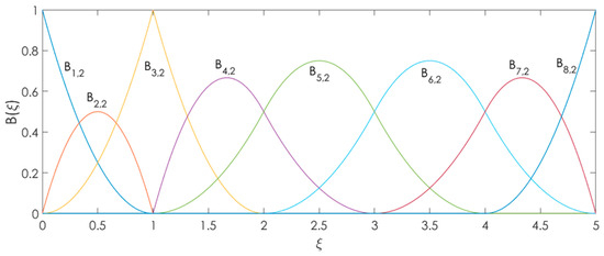
Figure 1.
B-spline basis functions with knot vector Ξ = {0,0,0,1,1,2,3,4,5,5,5}.
The NURBS (non-uniform rational B-spline) basis functions are determined by incorporating an ensemble of positive weights formulating the B-spline, .
NURBS (non-uniform rational B-spline) basis functions maintain continuity if there are no repeated internal knots. For a repeated knot of order k, the basis maintains continuity at the knot. An NURBS curve is described by the combination of NURBS basis functions of order p and n control points. Thus, it can be expressed as
The bivariate NURBS (2D) are defined as
In isogeometric analysis, the physical domain is represented on the right side, while the reference domain is depicted on the left side. The introduction of the reference domain helps simplify calculations involving matrix elements during the transition from the weak formulation to the matrix formulation. This simplification is achieved by utilizing numerical approximation methods, such as Gauss quadrature, to efficiently approximate integrals. By leveraging these techniques, the computational burden associated with the integration process is significantly reduced.
An extension of NURBS curves to NURBS surfaces and volumes is founded on tensor products of B-spline basis functions. NURBS surfaces are presented as follows:
Two parameter coordinates, (, ), are varied. The B-spline basis functions are defined for polynomial orders p and q, where m and n control points form the control net. Unlike tensor–product structures, the associated weights for the definition of NURBS basis functions are not bound by a predefined structure. They can be selected freely, similar to the selection of control points .
The derivatives of NURBS parametrizations with respect to the parameter coordinates can be obtained, which are straightforwardly valid for all orders of NURBS basis functions.
We follow a similar trajectory to [13], by introducing the extension of which verifies . From this, where .
Thus, problem (21) allows us to deduce that w is the solution of the following problem:
5. Numerical Results
In this section, we showcase numerical examples to illustrate the precision of the NURBS method in conjunction with the introduced finite elements from the preceding sections. Additionally, we present the numerical results obtained from our computational simulations, which aim to validate the accuracy and effectiveness of the chosen elements. To accomplish this, we employ a set of benchmark problems that have well-defined exact solutions. Furthermore, we explore the two-dimensional flow within a square domain.
It is important to emphasize that the NURBS-based isogeometric analysis (IGA) framework [15] offers significant advantages for studying two-dimensional lid-driven flow in one-quarter of an annulus. This is due to the inherent capability of NURBS to precisely represent complex geometries, in contrast to conventional finite element (FE) methods that only approximate the computational domain boundary. In our numerical simulations, we utilize the IGA library GeoPDEs [16], implemented in the MATLAB environment. By leveraging this framework, we can accurately capture the geometric features of the flow domain, allowing for a more faithful representation of the physical phenomena under investigation.
Throughout our computations, a global and uniform p-dependent stabilization parameter, denoted as C, is employed. The value of this parameter is determined by the expression where p represents the polynomial degree of the blending splines used in the approximation.
To assess the accuracy of the blending spline approximations, we compute the errors in two different norms L2 and :
These norms serve as quantitative measures of the discrepancy between the obtained approximations and the exact solutions. The computations are performed on a tensor product mesh, with the grid width h serving as a fundamental parameter in the error analysis [17].
- i.
- Numerical results on the unit square
Initially, we focus on investigating the Navier–Stokes problem within a two-dimensional domain [0, 1] × [0, 1]. This problem involves a source term denoted as f, which induces an analytical solution represented by the velocity components u = (, ) and the pressure field p
subject to the Dirichlet boundary conditions u = g, such that takes the values of the exact velocity solution on the boundary of the square.
The computational domain and the boundary conditions for the simulation of the flow are shown in Figure 2.
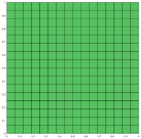
Figure 2.
A square geometry, defined as the set [0, 1] × [0, 1], and the control mesh of its NURBS representation 16 × 16.
The main purpose of using Dirichlet boundary conditions is as follows:
- Prescribed values: Dirichlet boundary conditions involve prescribing the values of certain flow variables (e.g., velocity, pressure, temperature) at the boundary. This allows the simulation to mimic real-world scenarios where specific boundary conditions are known or can be measured [18].
- Physical relevance: Dirichlet boundary conditions align with physical phenomena and constraints. They allow the simulation to capture the influence of real-world boundaries, such as walls or inlets/outlets, on the flow behavior. By imposing appropriate Dirichlet conditions, the flow near boundaries can be accurately represented, considering factors such as the no-slip condition on walls or prescribed inflow/outflow conditions at inlets and outlets.
- Ease of implementation: Dirichlet boundary conditions are easily implemented in numerical solvers. They do not require intricate mathematical formulations or additional equations compared to other boundary conditions.
Subsequently, we analyze the convergence of the error or the gap between the exact solution results and the NURBS method results, by generating error plots that illustrate the relationship between the error magnitude and the P parameter. These plots depict the convergence behavior and provide valuable insights into the accuracy and performance of our numerical method.
Observing the preceding figures, it is evident that the convergence of the and errors is highly apparent for various degree values of p. This mathematical plot implies the accuracy of the results obtained through the employment of the non-uniform rational B-splines (NURBS) methodology.
Depicted in Figure 3, Figure 4 and Figure 5, the error plots demonstrate a favorable convergence of the key parameters related to both the L2 and the H2 norms for various Re numbers. This convergence becomes evident as the mesh size of the square decreases, indicating an improvement in the accuracy of the results.
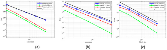
Figure 3.
Convergence of relative L2 error norm for different approaches with shape functions of order p: p = 1 (a), p = 2 (b), and p = 3 (c) at Re = 10.
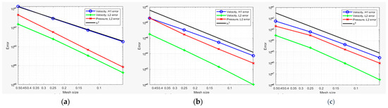
Figure 4.
Convergence of relative L2 error norm for different approaches with shape functions of order p: p = 1 (a), p = 2 (b), and p = 3 (c) at Re = 100.
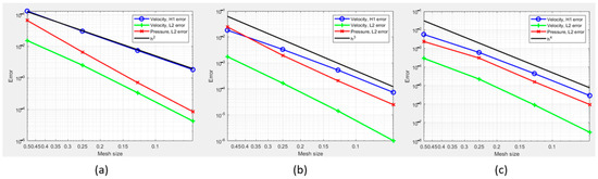
Figure 5.
Convergence of relative L2 error norm for different approaches with shape functions of order p: p = 1 (a), p = 2 (b), and p = 3 (c) at Re = 1000.
- ii.
- Benchmark NURBS and FEM for square example
In this section, our aim is to establish a benchmark for the non-uniform rational B-splines (NURBS) method as used in [19]. We achieve this by employing GEPDE’s code and incorporating the boundary conditions described in Section 4. Furthermore, we compare these results with those obtained through the finite element method (FEM) while utilizing the same set of boundary conditions at Reynolds number Re = 10.
- Velocity fields
Furthermore, in order to validate the quality of these results, it is crucial to conduct a comparison between the velocity field and the pressure field obtained from the NURBS/FEM and the exact solution defined in the previous section. By performing this comparative analysis, we can assess the accuracy and reliability of the NURBS method [20] in accurately representing the physical phenomena under consideration (see Figure 6).
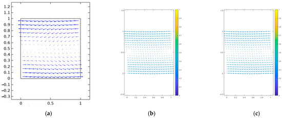
Figure 6.
Velocity vector field representation: FEM approximate solution (a), IGA approximate solution (b), and exact solution (c).
The obtained results clearly indicate a strong agreement between the NURBS method and the exact solution. This remarkable consistency substantiates the claim that the isogeometric analysis (IGA) method [12] is superior for such cases. Not only does it yield accurate outcomes, but it also exhibits a significant advantage in terms of computational efficiency, requiring less time to generate results. These findings emphasize the efficacy and practicality of employing the IGA method in similar scenarios.
- Pressure fields
Let us fix random points Ax = 0.0526 and Ay = 0.0526,
Let us examine the variation of the pressure field at a random point A and compare it with both the computed solution (NURBS) and the exact solution, as depicted in Figure 7.
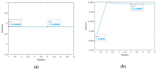
Figure 7.
The variation of the pressure field of the point A: (a) the computed solution (NURBS), and (b) the exact solution.
The plot demonstrates the method’s exceptional efficiency in terms of both data accuracy and time resolution, thanks to the minimal number of iterations (three) required for the result to stabilize.
The results of the pressure fields in the figure below show a very accurate concordance of the NURBS and exact solution (Figure 8).
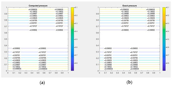
Figure 8.
Pressure field representation: IGA approximate solution (a), and exact solution (b).
For the finite element method (FEM), we plot the convergence of the total error in our domain with respect to the number of iterations required to achieve convergence for both the velocity field and the pressure field (Figure 9).
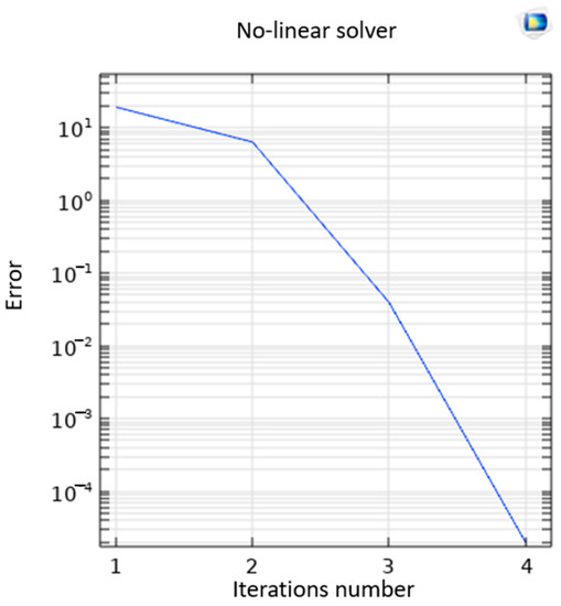
Figure 9.
The convergence of the FEM error regarding to the number of the iterations.
The error plot indicates that the results converge after four iterations, which means that the finite element method (FEM) is approximately 15% less efficient than isogeometric analysis (IGA) in terms of computation time.
6. Conclusions
In conclusion, the benchmarking of the non-uniform rational B-splines (NURBS) method [21], in conjunction with GEPDE’s code and the prescribed boundary conditions, produced highly promising results. The comparison of the velocity and pressure fields with the exact solution demonstrated a strong agreement, validating the accuracy and reliability of the NURBS method in representing the underlying physical phenomena.
Additionally, the NURBS method displayed superiority over the finite element method (FEM) in terms of computational efficiency, providing faster results without compromising accuracy, which is a critical factor for the computational market. These findings underscore the practicality and effectiveness of employing isogeometric analysis (IGA), particularly in cases where precise and efficient solutions are sought.
This study underscores the potential of the NURBS method and IGA in scientific analysis and computational modeling. Further exploration and research can be pursued to expand their applications across various domains and assess their performance in more complex scenarios.
Lastly, to further validate the effectiveness of the NURBS method, our future work will involve applying the same study to the non-linear Brinkman problem. By extending the analysis to porous media cases, we aim to assess the applicability and reliability of the NURBS method in capturing complex flow and transport phenomena. This investigation will offer valuable insights into the versatility and robustness of the NURBS method, expanding its potential applications in porous media simulations.
In our upcoming publication, we aim to improve the use of a mathematical technique called isogeometric non-uniform rational B-splines (NURBS) for studying porous materials. We specifically focus on solving a complex equation known as the Brinkman equation to describe the fluid flow in porous media. To achieve this, we adapt and employ a method called mixed web-spline finite element method [22,23] for the fluid dynamic problems, as well as the techniques of finite element method (FEM) used in recent papers [24,25,26,27], which may help us to find more accurate and reliable solutions to the problem at hand.
Author Contributions
Methodology, S.G., M.L.S. and S.V.; software, O.K.; writing—original draft, S.G.; writing—review and editing, S.G., M.L.S., S.V., A.E.A., A.E., O.K. and L.E.O. All authors have read and agreed to the published version of the manuscript.
Funding
This research received no external funding.
Data Availability Statement
All data generated or analyzed during this study are included in this paper.
Conflicts of Interest
The authors declare no conflict of interest.
References
- Li, D.; Luo, K.; Fan, J. Modulation of turbulence by dispersed solid particles in a spatially developing flat-plate boundary layer. J. Fluid Mech. 2016, 802, 359–394. [Google Scholar] [CrossRef]
- Argilaga, A.; Desrues, J.; Pont, S.; Combe, G.; Caillerie, D. FEM×DEM multiscale modeling: Model performance enhancement from Newton strategy to element loop parallelization. Int. J. Numer. Methods Eng. 2018, 114, 47–65. [Google Scholar] [CrossRef]
- Caglar, N.; Caglar, H. B-spline method for solving linear system of second-order boundary value problems. Comput. Math. Appl. Comput. Math. Appl. 2009, 57, 757–762. [Google Scholar] [CrossRef]
- Vázquez, R. A new design for the implementation of isogeometric analysis in Octave and Matlab: GeoPDEs 3.0. Comput. Math. Appl. 2016, 72, 523–554. [Google Scholar] [CrossRef]
- Klein, B.; Kummer, F.; Oberlack, M. ASIMPLE based discontinuous Galerkin solver for steady incompressible flows. J. Comput. Phys. 2013, 237, 235–250. [Google Scholar] [CrossRef]
- Dempsey, L.; Deguchi, K.; Hall, P.; Walton, A. Localized vortex/Tollmien–Schlichting wave interaction states in plane Poiseuille flow. J. Fluid Mech. 2016, 791, 97–121. [Google Scholar] [CrossRef][Green Version]
- Piasecki, T.; Pokorný, M. On steady solutions to a model of chemically reacting heat conducting compressible mixture with slip boundary conditions. In Mathematical Analysis in Fluid Mechanics: Selected Recent Results. International Conference on Vorticity, Rotation and Symmetry: Complex Fluids and the Issue of Regularity; American Mathematical Society: Providence, RI, USA, 2018. [Google Scholar] [CrossRef]
- El Moutea, O.; El Amri, H.; El Akkad, A. Finite Element Method for the Stokes–Darcy Problem with a New Boundary Condition. Numer. Anal. Appl. 2020, 13, 136–151. [Google Scholar] [CrossRef]
- El-Mekkaoui, J.; Elkhalfi, A.; Elakkad, A. Resolution of Stokes Equations with the Ca, b Boundary Condition Using Mixed Finite Element Method. WSEAS Trans. Math. 2013, 12, 586–597. [Google Scholar]
- Farin, G. NURBS for Curve and Surface Design; Society for Industrial & Applied: New York, NY, USA, 1991; Available online: https://dl.acm.org/doi/abs/10.5555/531858 (accessed on 27 June 2023).
- Hughes, T.J.; Cottrell, J.A.; Bazilevs, Y. Isogeometric analysis: CAD, finite elements, NURBS, exact geometry and mesh refinement. Comput. Methods Appl. Mech. Engrg. 2005, 194, 4135–4195. [Google Scholar] [CrossRef]
- Hughes, A.; Reali, G. Sangalli, Efficient quadrature for NURBS-based isogeometric analysis. Comput. Methods Appl. Mech. Eng. 2010, 199, 301–313. [Google Scholar] [CrossRef]
- Boffi, D.; Brezzi, F.; Fortin, M. Mixed Finite Element Methods and Applications; Springer: Berlin/Heidelberg, Germany, 2013; Volume 44. [Google Scholar]
- Bressan, A.; Sangalli, G. Isogeometric Discretizations of the Stokes Problem: Stability Analysis by the Macroelement Technique. IMA J. Numer. Anal. 2013, 33, 629–651. [Google Scholar] [CrossRef]
- El Ouadefli, L.; El Akkad, A.; El Moutea, O.; Moustabchir, H.; Elkhalfi, A.; Luminița Scutaru, M.; Muntean, R. Numerical Simulation for Brinkman System with Varied Permeability Tensor. Mathematics 2022, 10, 3242. [Google Scholar] [CrossRef]
- De Falco, C.; Reali, A.; Vázquez, R. GeoPDEs: A Research Tool for Isogeometric Analysis of PDEs. Adv. Eng. Softw. 2011, 42, 1020–1034. [Google Scholar] [CrossRef]
- Elakkad, A.; Elkhalfi, A.; Guessous, N. An a Posteriori Error Estimate for Mixed Finite Element Approximations of the Navier-Stokes Equations. J. Korean Math. Soc. 2011, 48, 529–550. [Google Scholar] [CrossRef][Green Version]
- Evans, J.A.; Hughes, T.J.R. Isogeometric Divergence-Conforming B-Splines for the Unsteady Navier–Stokes Equations. J. Comput. Phys. 2013, 241, 141–167. [Google Scholar] [CrossRef]
- Hosseini, B.S.; Möller, M.; Turek, S. Isogeometric Analysis of the Navier–Stokes Equations with Taylor–Hood B-Spline Elements. Appl. Math. Comput. 2015, 267, 264–281. [Google Scholar] [CrossRef]
- Hosseini, B.S.; Turek, S.; Möller, M.; Palmes, C. Isogeometric Analysis of the Navier–Stokes–Cahn–Hilliard Equations with Application to Incompressible Two-Phase Flows. J. Comput. Phys. 2017, 348, 171–194. [Google Scholar] [CrossRef]
- Buffa, A.; Rivas, J.; Sangalli, G.; Vázquez, R. Isogeometric Discrete Differential Forms in Three Dimensions. SIAM J. Numer. Anal. 2011, 49, 818–844. [Google Scholar] [CrossRef]
- El Moutea, O.; El Ouadefli, L.; El Akkad, A.; Nakbi, N.; Elkhalfi, A.; Scutaru, M.L.; Vlase, S. A Posteriori Error Estimators for the Quasi-Newtonian Stokes Problem with a General Boundary Condition. Mathematics 2023, 11, 1943. [Google Scholar] [CrossRef]
- Koubaiti, O.; El Fakkoussi, S.; El-Mekaoui, J.; Moustabchir, H.; Elkhalfi, A.; Pruncu, C. The treatment of constraints due to standard boundary conditions in the context of the mixed Web-spline finite element method. Eng. Comput. 2021, 38, 2937–2968. [Google Scholar] [CrossRef]
- Montassir, S.; Yakoubi, K.; Moustabchir, H.; Elkhalfi, A.; Rajak, D.K.; Pruncu, C.I. Analysis of crack behaviour in pipeline system using FAD diagram based on numerical simulation under XFEM. Appl. Sci. 2020, 10, 6129. [Google Scholar] [CrossRef]
- El Fakkoussi, S.; Moustabchir, H.; Elkhalfi, A.; Pruncu, C.I. Computation of the stress intensity factor KI for external longitudinal semi-elliptic cracks in the pipelines by FEM and XFEM methods. Int. J. Interact. Des. Manuf. 2019, 13, 545–555. [Google Scholar] [CrossRef]
- Koubaiti, O.; Elkhalfi, A.; El-Mekkaoui, J.; Mastorakis, N. Solving the problem of constraints due to Dirichlet boundary conditions in the context of the mini element method. Int. J. Mech. 2020, 14, 12–22. [Google Scholar]
- Yakoubi, K.; Montassir, S.; Moustabchir, H.; Elkhalfi, A.; Pruncu, C.I.; Arbaoui, J.; Farooq, M.U. An extended finite element method (XFEM) study on the elastic t-stress evaluations for a notch in a pipe steel exposed to internal pressure. Mathematics 2021, 9, 507. [Google Scholar] [CrossRef]


Disclaimer/Publisher’s Note: The statements, opinions and data contained in all publications are solely those of the individual author(s) and contributor(s) and not of MDPI and/or the editor(s). MDPI and/or the editor(s) disclaim responsibility for any injury to people or property resulting from any ideas, methods, instructions or products referred to in the content. |
© 2023 by the authors. Licensee MDPI, Basel, Switzerland. This article is an open access article distributed under the terms and conditions of the Creative Commons Attribution (CC BY) license (https://creativecommons.org/licenses/by/4.0/).