Global Properties of HIV-1 Dynamics Models with CTL Immune Impairment and Latent Cell-to-Cell Spread

Abstract

This paper presents and analyzes two mathematical models for the human immunodeficiency virus type-1 (HIV-1) infection with Cytotoxic T Lymphocyte cell (CTL) immune impairment. These models describe the interactions between healthy CD$4^{+}$T cells, latently and actively infected cells, HIV-1 particles, and CTLs. The healthy CD$4^{+}$T cells might be infected when they make contact with: (i) HIV-1 particles due to virus-to-cell (VTC) contact; (ii) latently infected cells due to latent cell-to-cell (CTC) contact; and (iii) actively infected cells due to active CTC contact. Distributed time delays are considered in the second model. We show the nonnegativity and boundedness of the solutions of the systems. Further, we derive basic reproduction numbers ${\Re }_0$ and ${\tilde{\Re }}_0$, that determine the existence and stability of equilibria of our proposed systems. We establish the global asymptotic stability of all equilibria by using the Lyapunov method together with LaSalle’s invariance principle. We confirm the theoretical results by numerical simulations. The effect of immune impairment, time delay and CTC transmission on the HIV-1 dynamics are discussed. It is found that weak immunity contributes significantly to the development of the disease. Further, we have established that the presence of time delay can significantly decrease the basic reproduction number and then suppress the HIV-1 replication. On the other hand, the presence of latent CTC spread increases the basic reproduction number and then enhances the viral progression. Thus, neglecting the latent CTC spread in the HIV-1 infection model will lead to an underestimation of the basic reproduction number. Consequently, the designed drug therapies will not be accurate or sufficient to eradicate the viruses from the body. These findings may help to improve the understanding of the dynamics of HIV-1 within a host.

1. Introduction

Human immunodeficiency virus type-1 (HIV-1) is one of the chronic viruses that infects humans and causes Acquired Immune Deficiency Syndrome (AIDS). HIV-1 attacks the CD4${}^{+}$T cells which are essential in the immune system. Adaptive immune responses play pivotal roles in HIV infection. B cells and cytotoxic T lymphocytes (CTLs) are two potential components of the adaptive immune response. B cells produce antibodies to neutralize the HIV-1 particles, while CTLs kill cells infected by HIV-1. Evaluating interactions between HIV-1 and target cells as well as immune cells can be experimentally expensive. Thus, mathematical modeling of HIV-1 infection has become an important tool for understanding the dynamical behavior of the viruses and their interactions with target cells and immune cells. Nowak and Bangham [1] presented the primary HIV-1 dynamics model which involve three components: healthy CD4${}^{+}$T cells (H), infected CD4${}^{+}$T cells (Y) and free HIV-1 particles (V). In the same paper, the CTL immune response was modeled as:

$$\begin{array}{cc}\hfill \mathrm{Healthy}{\mathrm{CD}4}^{+}\mathrm{T}\mathrm{cells}& :\dot{H}\left(t\right)=\underset{\mathrm{Production}\mathrm{of}\mathrm{healthy}{\mathrm{CD}4}^{+}\mathrm{T}\mathrm{cells}}{\underbrace{\alpha }}-\underset{\mathrm{Natural}\mathrm{death}}{\underbrace{\eta H\left(t\right)}}-\underset{\mathrm{Infectious}\mathrm{transmission}}{\underbrace{{\rho }_{1}H\left(t\right)V\left(t\right)}},\hfill \\ \hfill \mathrm{Actively}\mathrm{infected}{\mathrm{CD}4}^{+}\mathrm{T}\mathrm{cells}& :\dot{Y}\left(t\right)=\underset{\mathrm{Infectious}\mathrm{transmission}}{\underbrace{{\rho }_{1}H\left(t\right)V\left(t\right)}}-\underset{\mathrm{Natural}\mathrm{death}}{\underbrace{\tau Y\left(t\right)}}-\underset{\mathrm{Killing}\mathrm{of}\mathrm{infected}\mathrm{cells}\mathrm{by}\mathrm{CTLs}}{\underbrace{\gamma I\left(t\right)Y\left(t\right)}},\hfill \\ \hfill \mathrm{HIV}-1\mathrm{particles}& :\dot{V}\left(t\right)=\underset{\mathrm{Burst}\mathrm{size}}{\underbrace{\epsilon Y\left(t\right)}}-\underset{\mathrm{Natural}\mathrm{death}}{\underbrace{\theta V\left(t\right)}},\hfill \end{array}$$

(1)

$$\begin{array}{cc}\hfill \mathrm{CTLs}& :\dot{I}\left(t\right)=\underset{\mathrm{CTLs}\mathrm{stimulation}}{\underbrace{\nu Y\left(t\right)I\left(t\right)}}-\underset{\mathrm{Natural}\mathrm{death}}{\underbrace{\pi I\left(t\right)}},\hfill \end{array}$$

(2)

where $I\left(t\right)$ is the concentration of the CTLs at time t. After introducing this model, several virus dynamics models were developed and studied. Let us write the population dynamics of the CTLs as:

$$\dot{I}\left(t\right)=\mathrm{\Theta }(Y\left(t\right),I\left(t\right))-\pi I\left(t\right),$$

where $\mathrm{\Theta }(Y,I)$ is the stimulation rate of CTLs. It has taken many shapes in the literature:

S1. 

Self-regulating CTL, $\mathrm{\Theta }(Y,I)=\omega$, where $\omega >0$ [2],

S2. 

Linear CTL response, $\mathrm{\Theta }(Y,I)=\lambda Y$, where $\lambda >0$ [3,4,5,6],

S3. 

Predator-prey-like CTL, $\mathrm{\Theta }(Y,I)=\nu YI$, where $\nu >0$ [1,2,7],

S4. 

Combination of shapes S1–S3, $\mathrm{\Theta }(Y,I)=\omega +\lambda Y+\nu YI$ [2],

S5. 

Combination of predator-prey-like CTL and self-proliferation CTL: $\mathrm{\Theta }(Y,I)=\nu YI+\varsigma I\left(1-\frac{I}{I_{max}}\right)$, where $\varsigma ,I_{max}>0$ [8].

S6. 

Saturated CTL response: $\mathrm{\Theta }(Y,I)=\frac{\nu YI}{\vartheta +I}$, $\vartheta >0$ [9,10,11,12].

Some important biological factors were not included in models (1) and (2), such as:

Latently infected cells: these cells are considered one of the main obstacles for eliminating the HIV-1 by current antiviral drug therapies. Such cells contain the HIV-1 virions but do not generate them until they are activated. HIV-1 infection models with CTL immunity and latently infected cells were introduced in other research papers (see, e.g., [7,13]).

Time delay: in [14], it was estimated that the time between the HIV-1 entering a CD$4^{+}$T cell until generating new HIV-1 particles is about 0.9 days. Viral infection models with both CTL immunity and time delays were introduced in several works (see, e.g., [15,16,17,18]).

Cell-to-cell (CTC) transmission: the above model assumes that the infection occurs via virus-to-cell (VTC) contact. However, several research works reported that HIV-1 can be directly transferred from an infected CD$4^{+}$T cell to a healthy CD$4^{+}$T cell through the formation of virological synapses (see, e.g., [19,20,21,22,23,24]). CTC has great influence on HIV-1 infection, which might be 100–1000 times faster than VTC virus spread [25]. In [26,27], viral infection models with latently infected cells and CTC transmission were studied.

Immune impairment: models (1) and (2) assume that the presence of an antigen can only simulate the immune CTL response, and neglect the CTL immune impairment. In fact, HIV-1 is one of the viruses that has the ability to suppress the CTL response and cause CTL immune impairment [28]. In this case, the pollution dynamics of the CTLs can be written as follows (see, e.g., [28,29,30,31,32,33,34,35]):

$$\dot{I}\left(t\right)=\lambda Y\left(t\right)-\delta I\left(t\right)Y\left(t\right)-\pi I\left(t\right),$$

where, $\lambda Y$ is the stimulation of CTL immunity and $\delta IY$ is the CTL immune impairment. Modeling the latently infected cells and CTL immune impairment was studied in [36,37]. Intracellular time delay was considered in [36], while CTL immune response delay was considered in [37].

A viral infection model with CTL immune impairment, latently infected cells and CTC transmission can be written as [38,39,40]:

$$\begin{array}{cc}\hfill \dot{H}\left(t\right)& =\alpha -\eta H\left(t\right)-{\rho }_{1}H\left(t\right)V\left(t\right)-{\rho }_{3}H\left(t\right)Y\left(t\right),\hfill \end{array}$$

(3)

$$\begin{array}{cc}\hfill \dot{S}\left(t\right)& ={\rho }_{1}H\left(t\right)V\left(t\right)+{\rho }_{3}H\left(t\right)Y\left(t\right)-\left(\sigma +\mu \right)S\left(t\right),\hfill \end{array}$$

(4)

$$\begin{array}{cc}\hfill \dot{Y}\left(t\right)& =\sigma S\left(t\right)-\tau Y\left(t\right)-\gamma I\left(t\right)Y\left(t\right),\hfill \end{array}$$

(5)

$$\begin{array}{cc}\hfill \dot{V}\left(t\right)& =\epsilon Y\left(t\right)-\theta V\left(t\right),\hfill \end{array}$$

(6)

$$\begin{array}{cc}\hfill \dot{I}\left(t\right)& =\lambda Y\left(t\right)-\pi I\left(t\right)-\delta I\left(t\right)Y\left(t\right),\hfill \end{array}$$

(7)

where, $S\left(t\right)$ is the concentration of the latently infected cells at time t. The healthy CD4${}^{+}$T cells become infected by two modes: the VTC infection mode via HIV-1, ${\rho }_{1}HV$ and the CTC infection mode via actively infected cells, ${\rho }_{3}HY$. Latently infected cells are activated at rate $\sigma S$ and die at rate $\mu S$. Elaiw et al. [41] studied a virus dynamics model with CTC infection, immune impairment and intracellular time delay. In [40], CTL immune response delay was included. Alofi and Azoz [39] studied a viral infection model with general VTC and CTC infection rates.

We noted that the models presented in [38,39,40] assume that the CTC transmission is only due to the actively infected cells. However, it was reported in Ref. [42] that latently infected cells can also infect the healthy CD$4^{+}$T cells through the CTC mechanism. In Refs. [43,44,45,46,47,48,49], some virus dynamics models were developed by assuming that both latently and actively infected cells contribute to the CTC mechanism. However, the immune impairment was not considered in these papers.

The aim of the present work is to study two within-host HIV-1 dynamics models by involving latently infected cells, CTL immune impairment and CTC transmission. Both latently and actively infected cells contribute in CTC infection. In the second model, we included three types of distributed time delays. For both models we are investigating the non-negativity and boundedness of solutions, calculating the basic reproduction number, finding the model’s equilibria, establishing the global stability of equilibria, confirming the theoretical results by numerical simulation and discussing the obtained results.

2. Model with Latent CTC Transmission and CTL Immune Impairment

2.1. System Description

We propose an HIV-1 dynamics model with immune impairment, latently infected cells and two modes of transmissions, namely VTC and CTC. Both latently and actively infected cells contribute to CTC infection. Under these assumptions, we present the following model:

$$\left\{\begin{array}{cc}\dot{H}\left(t\right)\hfill & =\alpha -\eta H\left(t\right)-{\rho }_{1}H\left(t\right)V\left(t\right)-{\rho }_{2}H\left(t\right)S\left(t\right)-{\rho }_{3}H\left(t\right)Y\left(t\right),\hfill \\ \dot{S}\left(t\right)\hfill & ={\rho }_{1}H\left(t\right)V\left(t\right)+{\rho }_{2}H\left(t\right)S\left(t\right)+{\rho }_{3}H\left(t\right)Y\left(t\right)-\left(\sigma +\mu \right)S\left(t\right),\hfill \\ \dot{Y}\left(t\right)\hfill & =\sigma S\left(t\right)-\tau Y\left(t\right)-\gamma I\left(t\right)Y\left(t\right),\hfill \\ \dot{V}\left(t\right)\hfill & =\epsilon Y\left(t\right)-\theta V\left(t\right),\hfill \\ \dot{I}\left(t\right)\hfill & =\lambda Y\left(t\right)-\pi I\left(t\right)-\delta I\left(t\right)Y\left(t\right).\hfill \end{array}\right.$$

(8)

In our proposed model we assume that the healthy CD4${}^{+}$T cells become infected by three rates: the VTC infection rate via HIV-1 particles, ${\rho }_{1}HV$, the CTC infection rate via latently infected cells, ${\rho }_{2}HS,$ and the CTC infection rate via actively infected cells, ${\rho }_{3}HY$.

2.2. Basic Properties

2.2.1. Nonnegativity and Boundedness of the Solutions

Lemma 1. 

Consider system (8), then there exists a positively invariant compact set

$$\mathrm{\Omega }=\left\{\left(H,S,Y,V,I\right)\in {\mathbb{R}}_{\ge 0}^5:0\le H\left(t\right),S\left(t\right),Y\left(t\right)\le {\mathrm{\Lambda }}_1,0\le V\left(t\right)\le {\mathrm{\Lambda }}_2,0\le I\left(t\right)\le {\mathrm{\Lambda }}_3\right\}.$$

Proof. 

We have

$$\begin{array}{cc}\hfill \dot{H}& {\mid }_{H=0}=\alpha >0,\hfill \\ \hfill \dot{S}& {\mid }_{S=0}={\rho }_{1}HV+{\rho }_{3}HY\ge 0,\mathrm{for}\mathrm{all}H,V,Y\ge 0,\hfill \\ \hfill \dot{Y}& {\mid }_{Y=0}=\sigma S\ge 0,\mathrm{for}\mathrm{all}S\ge 0,\hfill \\ \hfill \dot{V}& {\mid }_{V=0}=\epsilon Y\ge 0,\mathrm{for}\mathrm{all}Y\ge 0,\hfill \\ \hfill \dot{I}& {\mid }_{I=0}=\lambda Y\ge 0,\mathrm{for}\mathrm{all}Y\ge 0.\hfill \end{array}$$

Therefore, $(H\left(t\right),S\left(t\right),Y\left(t\right),V\left(t\right),I\left(t\right))\in {\mathbb{R}}_{\ge 0}^5$, for all $t\ge 0$ when $(H\left(0\right),S\left(0\right),Y\left(0\right),V\left(0\right),I\left(0\right))\in {\mathbb{R}}_{\ge 0}^5$. Now, we define

$$T\left(t\right)=H\left(t\right)+S\left(t\right)+Y\left(t\right)+\frac{\tau }{2\epsilon }V\left(t\right)+\frac{\tau }{4\lambda }I\left(t\right).$$

Then, we have

$$\begin{array}{cc}\hfill \dot{T}\left(t\right)& =\dot{H}\left(t\right)+\dot{S}\left(t\right)+\dot{Y}\left(t\right)+\frac{\tau }{2\epsilon }\dot{V}\left(t\right)+\frac{\tau }{4\lambda }\dot{I}\left(t\right)\hfill \\ \hfill & =\alpha -\eta H\left(t\right)-\mu S\left(t\right)-\frac{\tau }{4}Y\left(t\right)-\left(\gamma +\frac{\tau \delta }{4\lambda }\right)I\left(t\right)Y\left(t\right)-\frac{\tau \theta }{2\epsilon }V\left(t\right)-\frac{\tau \pi }{4\lambda }I\left(t\right)\hfill \\ \hfill & \le \alpha -\eta H\left(t\right)-\mu S\left(t\right)-\frac{\tau }{4}Y\left(t\right)-\frac{\tau \theta }{2\epsilon }V\left(t\right)-\frac{\tau \pi }{4\lambda }I\left(t\right)\hfill \\ \hfill & \le \alpha -\varphi \left(H\left(t\right)+S\left(t\right)+Y\left(t\right)+\frac{\tau }{2\epsilon }V\left(t\right)+\frac{\tau }{4\lambda }I\left(t\right)\right)=\alpha -\varphi T\left(t\right),\hfill \end{array}$$

where $\varphi =min\left\{\eta ,\mu ,\frac{\tau }{4},\theta ,\pi \right\}$. Hence,

$$T\left(t\right)\le e^{-\varphi t}\left(T\left(0\right)-\frac{\alpha }{\varphi }\right)+\frac{\alpha }{\varphi }.$$

This yields $0\le T\left(t\right)\le {\mathrm{\Lambda }}_1$ if $T\left(0\right)\le {\mathrm{\Lambda }}_1$, where ${\mathrm{\Lambda }}_1={\displaystyle \frac{\alpha }{\varphi }}$. Since all state variables are nonnegative, then $0\le H\left(t\right),S\left(t\right),Y\left(t\right)\le {\mathrm{\Lambda }}_1$, $0\le V\left(t\right)\le {\mathrm{\Lambda }}_2$, and $0\le I\left(t\right)\le {\mathrm{\Lambda }}_3$, for all $t\ge 0$ if $H\left(0\right)+S\left(0\right)+Y\left(0\right)+{\displaystyle \frac{\tau }{2\epsilon }}V\left(0\right)+{\displaystyle \frac{\tau }{4\lambda }}I\left(0\right)\le {\mathrm{\Lambda }}_1$, where ${\mathrm{\Lambda }}_2={\displaystyle \frac{2\epsilon {\mathrm{\Lambda }}_1}{\tau }}$ and ${\mathrm{\Lambda }}_3={\displaystyle \frac{4\lambda {\mathrm{\Lambda }}_1}{\tau }}.$ Therefore, $H\left(t\right)$,$S\left(t\right)$,$Y\left(t\right)$,$V\left(t\right)$ and $I\left(t\right)$ are all bounded, which implies that $\mathrm{\Omega }$ is a positively invariant compact set with respect to system (8). □

2.2.2. Reproduction Number and Equilibria

Lemma 2. 

For system (8), there exists a positive basic reproduction number ${\Re }_0$ such that

(i) 

there exists only one equilibrium point $Q_0$ when ${\Re }_0\le 1$, and

(ii) 

there exists two equilibria $Q_0$ and $Q_1$ when ${\Re }_0>1.$

Proof. 

It is clear that system (8) always admits an infection-free equilibrium $Q_0=\left(H_0,0,0,0,0\right)$, where $H_0={\displaystyle \frac{\alpha }{\eta }}.$ Now, we apply the method of the next-generation matrix proposed in [50] to determine the basic reproduction number of system (8) based on the infected compartments in model (8), ordered $\left(S,Y,V\right).$ The nonlinear terms with new infection ${\widehat{\mathrm{\Gamma }}}_1$ and the outflow term ${\widehat{\Delta }}_1$ are given by the following matrices:

$$\begin{array}{cc}{\widehat{\mathrm{\Gamma }}}_1=\left(\begin{array}{c}{\rho }_{1}HV+{\rho }_{2}HS+{\rho }_{3}HY\\ 0\\ 0\end{array}\right),& {\widehat{\Delta }}_1=\left(\begin{array}{c}\left(\sigma +\mu \right)S\\ -\sigma S+\tau Y+\gamma IY\\ -\epsilon Y+\theta V\end{array}\right).\end{array}$$

We compute the derivative of ${\widehat{\mathrm{\Gamma }}}_1$ and ${\widehat{\Delta }}_1$ at the equilibrium $Q_0$ to obtain the following matrices:

$$\begin{array}{cc}{\mathrm{\Gamma }}_1=\left(\begin{array}{ccc}{\rho }_2{H}_0& {\rho }_3{H}_0& {\rho }_1{H}_0\\ 0& 0& 0\\ 0& 0& 0\end{array}\right),& {\Delta }_1=\left(\begin{array}{ccc}\sigma +\mu & 0& 0\\ -\sigma & \tau & 0\\ 0& -\epsilon & \theta \end{array}\right).\end{array}$$

Note that the next generation matrix is in the following form:

$${\mathrm{\Gamma }}_1{\Delta }_1^{-1}=\left(\begin{array}{ccc}\frac{H_0\left({\rho }_1\epsilon \sigma +{\rho }_2\theta \tau +{\rho }_3\sigma \theta \right)}{\left(\sigma +\mu \right)\theta \tau }& \frac{H_0\left({\rho }_1\epsilon +{\rho }_3\theta \right)}{\theta \tau }& \frac{{\rho }_1{H}_0}{\theta }\\ 0& 0& 0\\ 0& 0& 0\end{array}\right).$$

The basic reproduction number ${\Re }_0$ is the spectral radius of the matrix ${\mathrm{\Gamma }}_1{\Delta }_1^{-1}$ and is given as:

$${\Re }_0=\frac{H_0\left({\rho }_1\epsilon \sigma +{\rho }_2\theta \tau +{\rho }_3\sigma \theta \right)}{\left(\sigma +\mu \right)\theta \tau }={\Re }_{01}+{\Re }_{02}+{\Re }_{03},$$

(9)

where

$${\Re }_{01}={\displaystyle \frac{H_0\epsilon \sigma {\rho }_1}{\theta \tau \left(\sigma +\mu \right)}},{\Re }_{02}={\displaystyle \frac{H_0{\rho }_2}{\sigma +\mu }},{\Re }_{03}={\displaystyle \frac{H_0\sigma {\rho }_3}{\tau \left(\sigma +\mu \right)}}.$$

Note that the parameter ${\Re }_{01}$ measures the average number of secondary infected cells caused by the contact between the virus particles and the healthy cells, while ${\Re }_{02}$ and ${\Re }_{03}$ measure the average number of secondary infected cells caused by surviving latently and actively infected cells, respectively. To find the other equilibrium in addition to $Q_0$, we let $\left(H,S,Y,V,I\right)$ be any equilibrium satisfying the following equations:

$$\begin{array}{cc}\hfill 0& =\alpha -\eta H-{\rho }_{1}HV-{\rho }_{2}HS-{\rho }_{3}HY,\hfill \end{array}$$

(10)

$$\begin{array}{cc}\hfill 0& ={\rho }_{1}HV+{\rho }_{2}HS+{\rho }_{3}HY-\left(\sigma +\mu \right)S,\hfill \end{array}$$

(11)

$$\begin{array}{cc}\hfill 0& =\sigma S-\tau Y-\gamma IY,\hfill \end{array}$$

(12)

$$\begin{array}{cc}\hfill 0& =\epsilon Y-\theta V,\hfill \end{array}$$

(13)

$$\begin{array}{cc}\hfill 0& =\lambda Y-\pi I-\delta IY.\hfill \end{array}$$

(14)

From Equations (13) and (14), we obtain

$$V=\frac{\epsilon Y}{\theta },I=\frac{\lambda Y}{\pi +\delta Y}.$$

(15)

Substituting from Equation (15) into Equation (12), we obtain

$$S=\frac{\pi \tau Y+\left(\gamma \lambda +\tau \delta \right)Y^2}{\sigma \left(\pi +\delta Y\right)}.$$

(16)

From Equations (10) and (11), we obtain

$$\alpha -\eta H=\left(\sigma +\mu \right)S.$$

(17)

Substituting from Equation (16) into Equation (17), we obtain

$$H=\frac{1}{\eta }\left(\alpha -\frac{\left(\sigma +\mu \right)\left(\pi \tau Y+\left(\gamma \lambda +\tau \delta \right)Y^2\right)}{\sigma \left(\pi +\delta Y\right)}\right).$$

(18)

Substituting from Equations (15), (16) and (18) into Equation (11), we obtain

$$\frac{\eta \theta Y}{\sigma {\left(\pi +\delta Y\right)}^2}\left(A{Y}^3+B{Y}^2+CY+D\right)=0,$$

(19)

where

$$\begin{array}{cc}\hfill A& =\left(\sigma +\mu \right)\left(\gamma \lambda +\delta \tau \right)\left(\theta {\rho }_2\left(\delta \tau +\gamma \lambda \right)+\delta \sigma \left(\epsilon {\rho }_1+\theta {\rho }_3\right)\right),\hfill \\ \hfill B& =\delta \eta \theta \left(\sigma +\mu \right)\left(\gamma \lambda +\delta \tau \right)+\left(\pi \tau \left(\sigma +\mu \right)-\alpha \delta \right)\left(\delta \sigma \left(\epsilon {\rho }_1+\theta {\rho }_3\right)+\theta \left(\gamma \lambda +\delta \tau \right){\rho }_2\right)\hfill \\ \hfill & +\pi \left(\sigma +\mu \right)\left(\gamma \lambda +\delta \tau \right)\left(\epsilon \sigma {\rho }_1+\theta \left(\tau {\rho }_2+\sigma {\rho }_3\right)\right),\hfill \\ \hfill C& =\eta \theta \pi \left(\sigma +\mu \right)\left(2\delta \tau +\gamma \lambda \right)-\alpha \pi \left(\delta \sigma \left(\epsilon {\rho }_1+\theta {\rho }_3\right)+\theta \left(\gamma \lambda +\delta \tau \right){\rho }_2\right)\hfill \\ \hfill & +\pi \left(\pi \tau \left(\sigma +\mu \right)-\alpha \delta \right)\left(\epsilon \sigma {\rho }_1+\theta \left(\tau {\rho }_2+\sigma {\rho }_3\right)\right),\hfill \\ \hfill D& =\eta \theta \tau {\pi }^2\left(\sigma +\mu \right)\left(1-{\Re }_0\right),\hfill \end{array}$$

where ${\Re }_0$ is defined by Equation (9). From Equation (19), we have

• If $Y=0$, then from Equations (15), (16) and (18) we obtain the infection-free equilibrium $Q_0$.
• If $Y\ne 0$, then we have $A{Y}^3+B{Y}^2+CY+D=0$. In this case, let us define a function $\mathrm{\Psi }\left(Y\right)$ on $[0,\infty )$ as:

  $$\mathrm{\Psi }\left(Y\right)=A{Y}^3+B{Y}^2+CY+D.$$
  We have $\mathrm{\Psi }\left(0\right)=\eta \theta \tau {\pi }^2\left(\sigma +\mu \right)\left(1-{\Re }_0\right)<0$ when ${\Re }_0>1$ and $\underset{Y\to \infty }{lim}\mathrm{\Psi }\left(Y\right)=\infty$, which implies that $\mathrm{\Psi }$ has a positive real root $Y_1$. Then, by substituting from Equations (15) and (16) into Equation (10), we obtain

  $$H_1=\frac{\alpha }{\eta +{\rho }_1{V}_1+{\rho }_2{S}_1+{\rho }_3{Y}_1},$$

  where

  $$S_1=\frac{\pi \tau Y_1+\left(\gamma \lambda +\delta \tau \right)Y_1^2}{\sigma \left(\pi +\delta Y_1\right)},V_1={\displaystyle \frac{\epsilon Y_1}{\theta }},I_1={\displaystyle \frac{\lambda Y_1}{\pi +\delta Y_1}}.$$

It is clear that the infected equilibrium $Q_1=\left(H_1,S_1,Y_1,V_1,I_1\right)$ exists when ${\Re }_0>1$. □

2.2.3. Stability of Equilibria $Q_0$ and $Q_1$

Theorem 1. 

If ${\Re }_0<1$, then the $Q_0$ of system (8) is locally asymptotically stable (L.A.S), and unstable when ${\Re }_0>1$.

Proof. 

Following the work by Willems [51], local asymptotic stability of equilibrium $Q_0$ is determined by the eigenvalues of its corresponding Jacobian matrix which is given by

$$J_1=\left(\begin{array}{ccccc}-\eta -{\rho }_{1}V-{\rho }_{2}S-{\rho }_{3}Y& -{\rho }_{2}H& -{\rho }_{3}H& -{\rho }_{1}H& 0\\ {\rho }_{1}V+{\rho }_{2}S+{\rho }_{3}Y& {\rho }_{2}H-\left(\sigma +\mu \right)& {\rho }_{3}H& {\rho }_{1}H& 0\\ 0& \sigma & -\left(\tau +\gamma I\right)& 0& -\gamma Y\\ 0& 0& \epsilon & -\theta & 0\\ 0& 0& \lambda -\delta I& 0& -\left(\pi +\delta Y\right)\end{array}\right).$$

(20)

For matrix (20), the characteristic equation $\left|J_1-x{I}_5\right|=0$ is solved as $\left(x+\pi \right)\left(x+\eta \right)K\left(x\right)=0,$ where

$$K\left(x\right)=x^3+m_2{x}^2+m_{1}x+m_0,$$

(21)

and

$$\begin{array}{cc}\hfill & m_0=\theta \tau \left(\sigma +\mu \right)\left(1-{\Re }_0\right)>0,\hfill \\ \hfill & m_1=\theta \tau +\theta \left(\sigma +\mu \right)\left(1-{\Re }_{02}\right)+\tau \left(\sigma +\mu \right)\left(1-\left({\Re }_{02}+{\Re }_{03}\right)\right)>0,\hfill \\ \hfill & m_2=\theta +\tau +\left(\sigma +\mu \right)\left(1-{\Re }_{02}\right)>0,\hfill \\ \hfill & m_1{m}_2-m_0=\frac{\alpha \epsilon \sigma {\rho }_1}{\eta }+\left(\tau +\left(\sigma +\mu \right)\left(1-{\Re }_{02}\right)\right)\left(\theta (\theta +\tau )+\theta \left(\sigma +\mu \right)\left(1-{\Re }_{02}\right)\right.\hfill \\ \hfill & \left.+\tau \left(\sigma +\mu \right)\left(1-\left({\Re }_{02}+{\Re }_{03}\right)\right)\right)>0,\hfill \end{array}$$

where ${\Re }_0<1$. It is clear that the Jacobian matrix $J_1$ has two negative eigenvalues, $-\pi$ and $-\eta$. Other eigenvalues are calculated as the roots of the cubic equation presented in (21). All roots of Equation (21) have negative real parts based on Routh-Hurwitz criteria [51]. Therefore, the infection-free equilibrium $Q_0$ is L.A.S when ${\Re }_0<1$. Let ${\Re }_0>1$, then we have $m_0<0$. This means that Equation (21) has at least one positive real root. Hence, $Q_0$ is unstable when ${\Re }_0>1$. □

In the following theorems, global stability of equilibria will be discussed. Let a function $F$ be defined as $F\left(z\right)=z-1-ln\left(z\right)$. Denote $\left(H,S,Y,V,I\right)=\left(H\left(t\right),S\left(t\right),Y\left(t\right),V\left(t\right),I\left(t\right)\right).$

Theorem 2. 

For system (8), if ${\Re }_0<1$, then $Q_0$ is globally asymptotically stable (G.A.S).

Proof. 

We define a Lyapunov function candidate as:

$${\mathrm{\Theta }}_0=H_{0}F\left(\frac{H}{H_0}\right)+S+\frac{\left(\sigma +\mu \right)\left(1-{\Re }_{02}\right)}{\sigma }Y+\frac{{\rho }_1{H}_0}{\theta }V+\frac{\tau \left(\sigma +\mu \right)\left(1-{\Re }_0\right)}{\lambda \sigma }I.$$

Clearly, ${\mathrm{\Theta }}_0(H,S,Y,V,I)>0$ for all $H,S,Y,V,I>0$, and ${\mathrm{\Theta }}_0(H_0,0,0,0,0)=0$. We calculate $\frac{d{\mathrm{\Theta }}_0}{dt}$ along the solutions of model (8) as:

$$\begin{array}{cc}\hfill \frac{d{\mathrm{\Theta }}_0}{dt}& =\left(1-\frac{H_0}{H}\right)\frac{dH}{dt}+\frac{dS}{dt}+\frac{\left(\sigma +\mu \right)\left(1-{\Re }_{02}\right)}{\sigma }\frac{dY}{dt}+\frac{{\rho }_1{H}_0}{\theta }\frac{dV}{dt}+\frac{\tau \left(\sigma +\mu \right)\left(1-{\Re }_0\right)}{\lambda \sigma }\frac{dI}{dt}\hfill \\ \hfill & =\left(1-\frac{H_0}{H}\right)\left(\alpha -\eta H-{\rho }_{1}HV-{\rho }_{2}HS-{\rho }_{3}HY\right)+{\rho }_{1}HV+{\rho }_{2}HS+{\rho }_{3}HY-\left(\sigma +\mu \right)S\hfill \\ \hfill & +\frac{\left(\sigma +\mu \right)\left(1-{\Re }_{02}\right)}{\sigma }\left(\sigma S-\tau Y-\gamma IY\right)+\frac{{\rho }_1{H}_0}{\theta }\left(\epsilon Y-\theta V\right)+\frac{\tau \left(\sigma +\mu \right)\left(1-{\Re }_0\right)}{\lambda \sigma }\left(\lambda Y-\pi I-\delta IY\right)\hfill \\ \hfill & =\left(1-\frac{H_0}{H}\right)\left(\alpha -\eta H\right)+\left({\rho }_2{H}_0-\left(\sigma +\mu \right)+\left(\sigma +\mu \right)\left(1-{\Re }_{02}\right)\right)S\hfill \\ \hfill & +\left({\rho }_3{H}_0-\frac{\tau \left(\sigma +\mu \right)\left(1-{\Re }_{02}\right)}{\sigma }+\frac{{\rho }_1{H}_0\epsilon }{\theta }+\frac{\tau \left(\sigma +\mu \right)\left(1-{\Re }_0\right)}{\sigma }\right)Y\hfill \\ \hfill & -\frac{\pi \tau \left(\sigma +\mu \right)\left(1-{\Re }_0\right)}{\lambda \sigma }I-\left(\frac{\gamma \left(\sigma +\mu \right)\left(1-{\Re }_{02}\right)}{\sigma }+\frac{\delta \tau \left(\sigma +\mu \right)\left(1-{\Re }_0\right)}{\lambda \sigma }\right)IY.\hfill \end{array}$$

After direct calculation and using $H_0=\alpha /\eta$, we obtain

$$\begin{array}{cc}\hfill \frac{d{\mathrm{\Theta }}_0}{dt}& =\left(1-\frac{H_0}{H}\right)\left(\eta H_0-\eta H\right)-\frac{\pi \tau \left(\sigma +\mu \right)\left(1-{\Re }_0\right)}{\lambda \sigma }I-\frac{\sigma +\mu }{\lambda \sigma }\left(\gamma \lambda \left(1-{\Re }_{02}\right)+\tau \delta \left(1-{\Re }_0\right)\right)IY\hfill \\ \hfill & =-\frac{\eta {\left(H-H_0\right)}^2}{H}-\frac{\pi \tau \left(\sigma +\mu \right)\left(1-{\Re }_0\right)}{\lambda \sigma }I-\frac{\sigma +\mu }{\lambda \sigma }\left(\gamma \lambda \left(1-{\Re }_{02}\right)+\tau \delta \left(1-{\Re }_0\right)\right)IY.\hfill \end{array}$$

Clearly, $\frac{d{\mathrm{\Theta }}_0}{dt}\le 0$ when ${\Re }_0<1$ with equality holding when $H=H_0$ and $Y=I=0.$ Let ${\mathrm{\Phi }}_0=\left\{\left(H,S,Y,V,I\right):\frac{d{\mathrm{\Theta }}_0}{dt}=0\right\},$ and ${\mathrm{\Phi }}_0^{{}^{\prime }}$ be the largest invariant subset of ${\mathrm{\Phi }}_0$. Therefore, all solutions converge to ${\mathrm{\Phi }}_0^{{}^{\prime }}$ [52]. All elements in ${\mathrm{\Phi }}_0^{{}^{\prime }}$ satisfy $H\left(t\right)=H_0$ and $Y\left(t\right)=I\left(t\right)=0.$ Then, the third equation of system (8) gives

$$0=\dot{Y}\left(t\right)=\sigma S\left(t\right)⟹S\left(t\right)=0,\mathrm{for}\mathrm{all}t.$$

Moreover, the first equation of model (8) yields

$$0=\dot{H}\left(t\right)=\alpha -\eta H_0-{\rho }_1{H}_{0}V\left(t\right)⟹V\left(t\right)=0,\mathrm{for}\mathrm{all}t.$$

Therefore, ${\mathrm{\Phi }}_0^{{}^{\prime }}=\left\{\left(H,S,Y,V,I\right)\in {\mathrm{\Phi }}_0:H=H_0,S=Y=V=I=0\right\}=\left\{Q_0\right\}.$ Hence, we obtain that when ${\Re }_0<1$, then $Q_0$ is G.A.S according to the LaSalle’s invariance principle (L.I.P) [52]. □

Theorem 3. 

For system (8), if ${\Re }_0>1$, then $Q_1$ is G.A.S.

Proof. 

Define

$$\begin{array}{cc}\hfill {\mathrm{\Theta }}_1& =H_{1}F\left(\frac{H}{H_1}\right)+S_{1}F\left(\frac{S}{S_1}\right)+\frac{H_1\left({\rho }_1\epsilon +{\rho }_3\theta \right)Y_1}{\theta \left(\tau +\gamma I_1\right)}F\left(\frac{Y}{Y_1}\right)+\frac{{\rho }_1{H}_1{V}_1}{\theta }F\left(\frac{V}{V_1}\right)\hfill \\ \hfill & +\frac{\gamma H_1\left({\rho }_1\epsilon +{\rho }_3\theta \right)}{2\theta \left(\tau +\gamma I_1\right)\left(\lambda -\delta I_1\right)}{\left(I-I_1\right)}^2.\hfill \end{array}$$

It is noted from the equilibrium condition Equation (14) that $\lambda -\delta I_1={\displaystyle \frac{\pi I_1}{Y_1}}>0.$ Clearly, ${\mathrm{\Theta }}_1$ is positive definite. We calculate $\frac{d{\mathrm{\Theta }}_1}{dt}$ as:

$$\begin{array}{cc}\hfill \frac{d{\mathrm{\Theta }}_1}{dt}& =\left(1-\frac{H_1}{H}\right)\frac{dH}{dt}+\left(1-\frac{S_1}{S}\right)\frac{dS}{dt}+\frac{H_1\left({\rho }_1\epsilon +{\rho }_3\theta \right)}{\theta \left(\tau +\gamma I_1\right)}\left(1-\frac{Y_1}{Y}\right)\frac{dY}{dt}+\frac{{\rho }_1{H}_1}{\theta }\left(1-\frac{V_1}{V}\right)\frac{dV}{dt}\hfill \\ \hfill & +\frac{\gamma H_1\left({\rho }_1\epsilon +{\rho }_3\theta \right)}{\theta \left(\tau +\gamma I_1\right)\left(\lambda -\delta I_1\right)}\left(I-I_1\right)\frac{dI}{dt}\hfill \\ \hfill & =\left(1-\frac{H_1}{H}\right)\left(\alpha -\eta H-{\rho }_{1}HV-{\rho }_{2}HS-{\rho }_{3}HY\right)+\left(1-\frac{S_1}{S}\right)\left({\rho }_{1}HV+{\rho }_{2}HS+{\rho }_{3}HY\right.\hfill \\ \hfill & \left.-\left(\sigma +\mu \right)S\right)+\frac{H_1\left({\rho }_1\epsilon +{\rho }_3\theta \right)}{\theta \left(\tau +\gamma I_1\right)}\left(1-\frac{Y_1}{Y}\right)\left(\sigma S-\tau Y-\gamma IY\right)\hfill \\ \hfill & +\frac{{\rho }_1{H}_1}{\theta }\left(1-\frac{V_1}{V}\right)\left(\epsilon Y-\theta V\right)+\frac{\gamma H_1\left({\rho }_1\epsilon +{\rho }_3\theta \right)}{\theta \left(\tau +\gamma I_1\right)\left(\lambda -\delta I_1\right)}\left(I-I_1\right)\left(\lambda Y-\pi I-\delta IY\right)\hfill \\ \hfill & =\left(1-\frac{H_1}{H}\right)\left(\alpha -\eta H\right)+\left({\rho }_2{H}_1-\left(\sigma +\mu \right)+\frac{\sigma H_1\left({\rho }_1\epsilon +{\rho }_3\theta \right)}{\theta \left(\tau +\gamma I_1\right)}\right)S+{\rho }_3{H}_{1}Y\hfill \\ \hfill & -\left({\rho }_{1}HV+{\rho }_{2}HS+{\rho }_{3}HY\right)\left(\frac{S_1}{S}\right)+\left(\sigma +\mu \right)S_1-\frac{\sigma H_1\left({\rho }_1\epsilon +{\rho }_3\theta \right)}{\theta \left(\tau +\gamma I_1\right)}\left(\frac{S{Y}_1}{Y}\right)\hfill \\ \hfill & -\frac{\tau H_1\left({\rho }_1\epsilon +{\rho }_3\theta \right)}{\theta \left(\tau +\gamma I_1\right)}\left(Y-Y_1\right)-\frac{\gamma H_1\left({\rho }_1\epsilon +{\rho }_3\theta \right)}{\theta \left(\tau +\gamma I_1\right)}I\left(Y-Y_1\right)+\frac{{\rho }_1{H}_1\epsilon }{\theta }Y\hfill \\ \hfill & -\frac{{\rho }_1{H}_1\epsilon }{\theta }\left(\frac{Y{V}_1}{V}\right)+{\rho }_1{H}_1{V}_1+\frac{\gamma H_1\left({\rho }_1\epsilon +{\rho }_3\theta \right)}{\theta \left(\tau +\gamma I_1\right)\left(\lambda -\delta I_1\right)}\left(I-I_1\right)\left(\lambda Y-\pi I-\delta IY\right).\hfill \end{array}$$

(22)

Using the following equilibrium conditions for $Q_1$

$$\begin{array}{cc}\hfill & \alpha =\eta H_1+{\rho }_1{H}_1{V}_1+{\rho }_2{H}_1{S}_1+{\rho }_3{H}_1{Y}_1,\hfill \\ \hfill & {\rho }_1{H}_1{V}_1+{\rho }_2{H}_1{S}_1+{\rho }_3{H}_1{Y}_1=\left(\sigma +\mu \right)S_1,\hfill \\ \hfill & \sigma S_1=\left(\tau +\gamma I_1\right)Y_1⟹Y_1=\frac{\sigma S_1}{\tau +\gamma I_1},\hfill \\ \hfill & V_1=\frac{\epsilon Y_1}{\theta },\lambda Y_1-\pi I_1-\delta I_1{Y}_1=0,\hfill \end{array}$$

We obtain

$$\begin{array}{cc}\hfill & {\rho }_1{H}_1{V}_1+{\rho }_3{H}_1{Y}_1=\frac{H_1\left({\rho }_1\epsilon +{\rho }_3\theta \right)Y_1}{\theta }=\frac{\sigma H_1\left({\rho }_1\epsilon +{\rho }_3\theta \right)S_1}{\theta \left(\tau +\gamma I_1\right)},\hfill \\ \hfill & \left({\rho }_2{H}_1-\left(\sigma +\mu \right)+\frac{\sigma H_1\left({\rho }_1\epsilon +{\rho }_3\theta \right)}{\theta \left(\tau +\gamma I_1\right)}\right)S_1=0.\hfill \end{array}$$

Therefore, Equation (22) will take the following form:

$$\begin{array}{cc}\hfill \frac{d{\mathrm{\Theta }}_1}{dt}& =\left(1-\frac{H_1}{H}\right)\left(\eta H_1-\eta H\right)+\left({\rho }_1{H}_1{V}_1+{\rho }_2{H}_1{S}_1+{\rho }_3{H}_1{Y}_1\right)\left(1-\frac{H_1}{H}\right)+{\rho }_3{H}_{1}Y\hfill \\ \hfill & -{\rho }_1{H}_1{V}_1\left(\frac{HV{S}_1}{H_1{V}_{1}S}\right)-{\rho }_2{H}_1{S}_1\left(\frac{H}{H_1}\right)-{\rho }_3{H}_1{Y}_1\left(\frac{HY{S}_1}{H_1{Y}_{1}S}\right)+{\rho }_1{H}_1{V}_1+{\rho }_2{H}_1{S}_1\hfill \\ \hfill & +{\rho }_3{H}_1{Y}_1-\frac{\sigma H_1\left({\rho }_1\epsilon +{\rho }_3\theta \right)S_1}{\theta \left(\tau +\gamma I_1\right)}\left(\frac{S{Y}_1}{S_{1}Y}\right)-\frac{\tau H_1\left({\rho }_1\epsilon +{\rho }_3\theta \right)}{\theta \left(\tau +\gamma I_1\right)}\left(Y-Y_1\right)\hfill \\ \hfill & -\frac{\gamma H_1\left({\rho }_1\epsilon +{\rho }_3\theta \right)}{\theta \left(\tau +\gamma I_1\right)}I\left(Y-Y_1\right)+\frac{\gamma H_1\left({\rho }_1\epsilon +{\rho }_3\theta \right)}{\theta \left(\tau +\gamma I_1\right)}{I}_1\left(Y-Y_1\right)-\frac{\gamma H_1\left({\rho }_1\epsilon +{\rho }_3\theta \right)}{\theta \left(\tau +\gamma I_1\right)}{I}_1\left(Y-Y_1\right)\hfill \\ \hfill & +\frac{{\rho }_1{H}_1\epsilon Y_1}{\theta }\left(\frac{Y}{Y_1}\right)-\frac{{\rho }_1{H}_1\epsilon Y_1}{\theta }\left(\frac{Y{V}_1}{Y_{1}V}\right)+{\rho }_1{H}_1{V}_1+\frac{\gamma H_1\left({\rho }_1\epsilon +{\rho }_3\theta \right)}{\theta \left(\tau +\gamma I_1\right)\left(\lambda -\delta I_1\right)}\left(I-I_1\right)\left(\lambda Y-\pi I-\delta IY\right.\hfill \\ \hfill & \left.-\lambda Y_1+\pi I_1+\delta I_1{Y}_1+\delta I_{1}Y-\delta I_{1}Y\right)\hfill \\ \hfill & =-\frac{\eta {\left(H-H_1\right)}^2}{H}+\left({\rho }_1{H}_1{V}_1+{\rho }_2{H}_1{S}_1+{\rho }_3{H}_1{Y}_1\right)\left(2-\frac{H_1}{H}\right)+{\rho }_3{H}_{1}Y\hfill \\ \hfill & -{\rho }_1{H}_1{V}_1\left(\frac{HV{S}_1}{H_1{V}_{1}S}\right)-{\rho }_2{H}_1{S}_1\left(\frac{H}{H_1}\right)-{\rho }_3{H}_1{Y}_1\left(\frac{HY{S}_1}{H_1{Y}_{1}S}\right)-\left({\rho }_1{H}_1{V}_1+{\rho }_3{H}_1{Y}_1\right)\left(\frac{S{Y}_1}{S_{1}Y}\right)\hfill \\ \hfill & -\frac{H_1\left({\rho }_1\epsilon +{\rho }_3\theta \right)}{\theta \left(\tau +\gamma I_1\right)}\left(\tau +\gamma I_1\right)\left(Y-Y_1\right)-\frac{\gamma H_1\left({\rho }_1\epsilon +{\rho }_3\theta \right)}{\theta \left(\tau +\gamma I_1\right)}\left(I-I_1\right)\left(Y-Y_1\right)+{\rho }_1{H}_1{V}_1\left(\frac{Y}{Y_1}\right)\hfill \\ \hfill & -{\rho }_1{H}_1{V}_1\left(\frac{Y{V}_1}{Y_{1}V}\right)+{\rho }_1{H}_1{V}_1+\frac{\gamma \lambda H_1\left({\rho }_1\epsilon +{\rho }_3\theta \right)}{\theta \left(\tau +\gamma I_1\right)\left(\lambda -\delta I_1\right)}\left(I-I_1\right)\left(Y-Y_1\right)\hfill \\ \hfill & -\frac{\gamma H_1\left({\rho }_1\epsilon +{\rho }_3\theta \right)\left(\pi +\delta Y\right)}{\theta \left(\tau +\gamma I_1\right)\left(\lambda -\delta I_1\right)}{\left(I-I_1\right)}^2-\frac{\delta \gamma H_1\left({\rho }_1\epsilon +{\rho }_3\theta \right)I_1}{\theta \left(\tau +\gamma I_1\right)\left(\lambda -\delta I_1\right)}\left(I-I_1\right)\left(Y-Y_1\right).\hfill \end{array}$$

This implies that

$$\begin{array}{cc}\hfill \frac{d{\mathrm{\Theta }}_1}{dt}& =-\frac{\eta {\left(H-H_1\right)}^2}{H}+\left({\rho }_1{H}_1{V}_1+{\rho }_2{H}_1{S}_1+{\rho }_3{H}_1{Y}_1\right)\left(2-\frac{H_1}{H}\right)+{\rho }_3{H}_{1}Y\hfill \\ \hfill & -{\rho }_1{H}_1{V}_1\left(\frac{HV{S}_1}{H_1{V}_{1}S}\right)-{\rho }_2{H}_1{S}_1\left(\frac{H}{H_1}\right)-{\rho }_3{H}_1{Y}_1\left(\frac{HY{S}_1}{H_1{Y}_{1}S}\right)\hfill \\ \hfill & -\left({\rho }_1{H}_1{V}_1+{\rho }_3{H}_1{Y}_1\right)\left(\frac{S{Y}_1}{S_{1}Y}\right)-\frac{H_1\left({\rho }_1\epsilon +{\rho }_3\theta \right)}{\theta }\left(Y-Y_1\right)\hfill \\ \hfill & -\frac{\gamma H_1\left({\rho }_1\epsilon +{\rho }_3\theta \right)}{\theta \left(\tau +\gamma I_1\right)}\left(I-I_1\right)\left(Y-Y_1\right)+{\rho }_1{H}_1{V}_1\left(\frac{Y}{Y_1}\right)-{\rho }_1{H}_1{V}_1\left(\frac{Y{V}_1}{Y_{1}V}\right)+{\rho }_1{H}_1{V}_1\hfill \\ \hfill & +\frac{\gamma H_1\left({\rho }_1\epsilon +{\rho }_3\theta \right)}{\theta \left(\tau +\gamma I_1\right)\left(\lambda -\delta I_1\right)}\left(\lambda -\delta I_1\right)\left(I-I_1\right)\left(Y-Y_1\right)-\frac{\gamma H_1\left({\rho }_1\epsilon +{\rho }_3\theta \right)\left(\pi +\delta Y\right)}{\theta \left(\tau +\gamma I_1\right)\left(\lambda -\delta I_1\right)}{\left(I-I_1\right)}^2\hfill \\ \hfill & =-\frac{\eta {\left(H-H_1\right)}^2}{H}+\left({\rho }_1{H}_1{V}_1+{\rho }_2{H}_1{S}_1+{\rho }_3{H}_1{Y}_1\right)\left(2-\frac{H_1}{H}\right)+{\rho }_3{H}_{1}Y\hfill \\ \hfill & -{\rho }_1{H}_1{V}_1\left(\frac{HV{S}_1}{H_1{V}_{1}S}\right)-{\rho }_2{H}_1{S}_1\left(\frac{H}{H_1}\right)-{\rho }_3{H}_1{Y}_1\left(\frac{HY{S}_1}{H_1{Y}_{1}S}\right)\hfill \\ \hfill & -\left({\rho }_1{H}_1{V}_1+{\rho }_3{H}_1{Y}_1\right)\left(\frac{S{Y}_1}{S_{1}Y}\right)-\frac{H_1\left({\rho }_1\epsilon +{\rho }_3\theta \right)Y_1}{\theta }\left(\frac{Y}{Y_1}-1\right)+{\rho }_1{H}_1{V}_1\left(\frac{Y}{Y_1}\right)\hfill \\ \hfill & -{\rho }_1{H}_1{V}_1\left(\frac{Y{V}_1}{Y_{1}V}\right)+{\rho }_1{H}_1{V}_1-\frac{\gamma H_1\left({\rho }_1\epsilon +{\rho }_3\theta \right)\left(\pi +\delta Y\right)}{\theta \left(\tau +\gamma I_1\right)\left(\lambda -\delta I_1\right)}{\left(I-I_1\right)}^2\hfill \\ \hfill & =-\frac{\eta {\left(H-H_1\right)}^2}{H}+\left({\rho }_1{H}_1{V}_1+{\rho }_2{H}_1{S}_1+{\rho }_3{H}_1{Y}_1\right)\left(2-\frac{H_1}{H}\right)+{\rho }_3{H}_{1}Y\hfill \\ \hfill & -{\rho }_1{H}_1{V}_1\left(\frac{HV{S}_1}{H_1{V}_{1}S}\right)-{\rho }_2{H}_1{S}_1\left(\frac{H}{H_1}\right)-{\rho }_3{H}_1{Y}_1\left(\frac{HY{S}_1}{H_1{Y}_{1}S}\right)\hfill \\ \hfill & -\left({\rho }_1{H}_1{V}_1+{\rho }_3{H}_1{Y}_1\right)\left(\frac{S{Y}_1}{S_{1}Y}\right)-\left({\rho }_1{H}_1{V}_1+{\rho }_3{H}_1{Y}_1\right)\left(\frac{Y}{Y_1}-1\right)\hfill \\ \hfill & +{\rho }_1{H}_1{V}_1\left(\frac{Y}{Y_1}\right)-{\rho }_1{H}_1{V}_1\left(\frac{Y{V}_1}{Y_{1}V}\right)+{\rho }_1{H}_1{V}_1-\frac{\gamma H_1\left({\rho }_1\epsilon +{\rho }_3\theta \right)\left(\pi +\delta Y\right)}{\theta \left(\tau +\gamma I_1\right)\left(\lambda -\delta I_1\right)}{\left(I-I_1\right)}^2.\hfill \end{array}$$

Finally, we obtain

$$\begin{array}{cc}\hfill \frac{d{\mathrm{\Theta }}_1}{dt}& =-\frac{\left(\eta +{\rho }_2{S}_1\right){\left(H-H_1\right)}^2}{H}+{\rho }_1{H}_1{V}_1\left(4-\frac{H_1}{H}-\frac{HV{S}_1}{H_1{V}_{1}S}-\frac{S{Y}_1}{S_{1}Y}-\frac{Y{V}_1}{Y_{1}V}\right)\hfill \\ \hfill & +{\rho }_3{H}_1{Y}_1\left(3-\frac{H_1}{H}-\frac{HY{S}_1}{H_1{Y}_{1}S}-\frac{S{Y}_1}{S_{1}Y}\right)-\frac{\gamma H_1\left({\rho }_1\epsilon +{\rho }_3\theta \right)\left(\pi +\delta Y\right)}{\theta \left(\tau +\gamma I_1\right)\left(\lambda -\delta I_1\right)}{\left(I-I_1\right)}^2.\hfill \end{array}$$

The geometrical and arithmetical means relationship implies

$$\begin{array}{cc}\hfill 4& \le \frac{H_1}{H}+\frac{HV{S}_1}{H_1{V}_{1}S}+\frac{S{Y}_1}{S_{1}Y}+\frac{Y{V}_1}{Y_{1}V},\hfill \\ \hfill 3& \le \frac{H_1}{H}+\frac{HY{S}_1}{H_1{Y}_{1}S}+\frac{S{Y}_1}{S_{1}Y}.\hfill \end{array}$$

Hence, if ${\Re }_0>1$, then $\frac{d{\mathrm{\Theta }}_1}{dt}\le 0$ for all $H,S,Y,V,I>0$. Additionally, $\frac{d{\mathrm{\Theta }}_1}{dt}=0$ when $H=H_1,S=S_1,Y=Y_1,V=V_1$ and $I=I_1$. Let ${\mathrm{\Phi }}_1^{{}^{\prime }}$ be the largest invariant subset of ${\mathrm{\Phi }}_1=\left\{\left(H,S,Y,V,I\right):\frac{d{\mathrm{\Theta }}_1}{dt}=0\right\}$. Therefore, ${\mathrm{\Phi }}_1^{{}^{\prime }}=\left\{Q_1\right\}.$ Applying L.I.P, we obtain that if ${\Re }_0>1$, then $Q_1$ is G.A.S [52]. □

3. Model with Distributed Time Delays

3.1. System Description

In the following model, we consider the distributed time delays in system (8) to become represented by delay differential equations (DDEs):

$$\left\{\begin{array}{cc}\dot{H}\left(t\right)\hfill & =\alpha -\eta H\left(t\right)-{\rho }_{1}H\left(t\right)V\left(t\right)-{\rho }_{2}H\left(t\right)S\left(t\right)-{\rho }_{3}H\left(t\right)Y\left(t\right),\hfill \\ \dot{S}\left(t\right)\hfill & ={\int }_0^{k_1}{f}_1\left(\varrho \right)e^{-h_1\varrho }H\left(t-\varrho \right)\left({\rho }_{1}V\left(t-\varrho \right)+{\rho }_{2}S\left(t-\varrho \right)\right.\hfill \\ \hfill & \left.+{\rho }_{3}Y\left(t-\varrho \right)\right)d\varrho -(\sigma +\mu )S\left(t\right),\hfill \\ \dot{Y}\left(t\right)\hfill & =\sigma {\int }_0^{k_2}{f}_2\left(\varrho \right)e^{-h_2\varrho }S\left(t-\varrho \right)d\varrho -\tau Y\left(t\right)-\gamma I\left(t\right)Y\left(t\right),\hfill \\ \dot{V}\left(t\right)\hfill & =\epsilon {\int }_0^{k_3}{f}_3\left(\varrho \right)e^{-h_3\varrho }Y\left(t-\varrho \right)d\varrho -\theta V\left(t\right),\hfill \\ \dot{I}\left(t\right)\hfill & =\lambda Y\left(t\right)-\pi I\left(t\right)-\delta I\left(t\right)Y\left(t\right).\hfill \end{array}\right.$$

(23)

Here, $f_1\left(\varrho \right)e^{-h_1\varrho }$ demonstrates the probability that healthy CD4${}^{+}$T cells contacted by HIV-1 particles or infected cells at time $t-\varrho$ and after surviving $\varrho$ time units become latently infected cells at time t. The factor $f_2\left(\varrho \right)e^{-h_2\varrho }$ is the probability that latently infected cells after surviving $\varrho$ time units turned to actively infected cells at time t. Further, the factor $f_3\left(\varrho \right)e^{-h_3\varrho }$ represents the probability of new HIV-1 particles after surviving $\varrho$ time units and maturing at time t. Here, $h_i>0,$ $i=1,2,3$ are constants. $\varrho$ is the delay parameter taken from a probability distribution function $f_i\left(\varrho \right)$ over the interval $[0,k_i],$ $i=1,2,3,$ where $k_i$ is the limit superior of the delay period. Function $f_i\left(\varrho \right),$ $i=1,2,3$ satisfies the following conditions:

$$\begin{array}{cccccc}{f}_i\left(\varrho \right)>0,& {\int }_0^{k_i}{f}_i\left(\varrho \right)d\varrho =1,& \mathrm{and}& {\int }_0^{k_i}{f}_i\left(\varrho \right)e^{-\beta \varrho }d\varrho <\infty ,& \mathrm{where}& \beta >0.\end{array}$$

Let ${\overline{F}}_i\left(\varrho \right)=f_i\left(\varrho \right)e^{-h_i\varrho }$ and $F_i={\int }_0^{k_i}{\overline{F}}_i\left(\varrho \right)d\varrho ,$ $i=1,2,3.$ Therefore, $0<F_i\le 1,$ $i=1,2,3.$

The initial conditions of system (23) are:

$$\left\{\begin{array}{ccccc}H\left(r\right)=a_1\left(r\right),& S\left(r\right)=a_2\left(r\right),& Y\left(r\right)=a_3\left(r\right),& V\left(r\right)=a_4\left(r\right),& I\left(r\right)=a_5\left(r\right),\\ a_j\left(r\right)\ge 0,& j=1,2,\dots ,5,& r\in [-k,0],& k=max\{k_1,k_2,k_3\},\end{array}\right.$$

(24)

where $a_j\left(r\right)\in C([-k,0],{\mathbb{R}}_{\ge 0}),$ $j=1,2,\dots ,5$ and $C=$ $C\left(\left[-k,0\right],{\mathbb{R}}_{\ge 0}\right)$ is the Banach space of continuous functions with norm $∥a_j∥=\underset{-k\le \zeta \le 0}{sup}\left|a_j\left(\zeta \right)\right|$ for all $a_j\in C$. Therefore, system (23) with initial conditions (24) has a unique solution [52,53]. The biological meaning of all remaining variables and parameters follow the same identifications as given in Section 2.

3.2. Basic Properties

3.2.1. Nonnegativity and Ultimate Boundedness of the Solutions

Lemma 3. 

For system (23) together with initial conditions (24), there exists a compact set $\widehat{\mathrm{\Omega }}$ that is positively invariant, where

$$\widehat{\mathrm{\Omega }}=\{(H,S,Y,V,I)\in C_{\ge 0}^5:∥H\left(t\right)∥\le {\widehat{\mathrm{\Lambda }}}_1,∥S\left(t\right)∥\le {\widehat{\mathrm{\Lambda }}}_1,∥Y\left(t\right)∥\le {\widehat{\mathrm{\Lambda }}}_2,∥I\left(t\right)∥\le {\widehat{\mathrm{\Lambda }}}_3,∥V\left(t\right)∥\le {\widehat{\mathrm{\Lambda }}}_4\}.$$

Proof. 

In the beginning we show the nonnegativity of solutions. From the first equation of system (23), we have $\dot{H}{\mid }_{H=0}=\alpha >0,$ then $H\left(t\right)>0$, for all $t\ge 0.$ In addition, from the remaining equations of system (23) we have

$$\begin{array}{cc}\hfill & \dot{S}\left(t\right)+\left(\sigma +\mu \right)S\left(t\right)={\int }_0^{k_1}{\overline{F}}_1\left(\varrho \right)H\left(t-\varrho \right)\left({\rho }_{1}V\left(t-\varrho \right)+{\rho }_{2}S\left(t-\varrho \right)+{\rho }_{3}Y\left(t-\varrho \right)\right)d\varrho \hfill \\ \hfill & ⟹S\left(t\right)=a_2\left(0\right)e^{-(\sigma +\mu )t}+{\int }_0^t{e}^{-(\sigma +\mu )(t-\varkappa )}{\int }_0^{k_1}{\overline{F}}_1\left(\varrho \right)H\left(\varkappa -\varrho \right)({\rho }_{1}V\left(\varkappa -\varrho \right)\hfill \\ \hfill & +{\rho }_{2}S\left(\varkappa -\varrho \right)+{\rho }_{3}Y\left(\varkappa -\varrho \right))d\varrho d\varkappa \ge 0.\hfill \\ \hfill & \dot{Y}\left(t\right)+\left(\tau +\gamma I\left(t\right)\right)Y\left(t\right)=\sigma {\int }_0^{k_2}{\overline{F}}_2\left(\varrho \right)S\left(t-\varrho \right)d\varrho \hfill \\ \hfill & ⟹Y\left(t\right)=a_3\left(0\right)e^{-{\int }_0^t(\tau +\gamma I\left(u\right))du}+\sigma {\int }_0^t{e}^{-{\int }_{\varkappa }^t(\tau +\gamma I\left(u\right))du}{\int }_0^{k_2}{\overline{F}}_2\left(\varrho \right)S\left(\varkappa -\varrho \right)d\varrho d\varkappa \ge 0.\hfill \\ \hfill & \dot{V}\left(t\right)+\theta V\left(t\right)=\epsilon {\int }_0^{k_3}{\overline{F}}_3\left(\varrho \right)Y\left(t-\varrho \right)d\varrho \hfill \\ \hfill & ⟹V\left(t\right)=a_4\left(0\right)e^{-\theta t}+\epsilon {\int }_0^t{e}^{-\theta (t-\varkappa )}{\int }_0^{k_3}{\overline{F}}_3\left(\varrho \right)Y\left(\varkappa -\varrho \right)d\varrho d\varkappa \ge 0.\hfill \\ \hfill & \dot{I}\left(t\right)+\left(\pi +\delta Y\left(t\right)\right)I\left(t\right)=\lambda Y\left(t\right)\hfill \\ \hfill & ⟹I\left(t\right)=a_5\left(0\right)e^{-{\int }_0^t(\pi +\delta Y\left(u\right))du}+\lambda {\int }_0^t{e}^{-{\int }_{\varkappa }^t(\pi +\delta Y\left(u\right))du}Y\left(\varrho \right)d\varrho \ge 0,\hfill \end{array}$$

for all $t\in [0,k]$. Then, by a recursive argument we have $H\left(t\right),S\left(t\right),Y\left(t\right),V\left(t\right)$ and $I\left(t\right)$ are nonnegative for all $t\ge 0$. Therefore, the solutions of system (23) satisfy $\left(H\left(t\right),S\left(t\right),Y\left(t\right),V\left(t\right),I\left(t\right)\right)\in {\mathbb{R}}_{\ge 0}^5,$ for all $t\ge 0$. Next, we prove the ultimate boundedness of all solutions. From the first equation of system (23), we have $\underset{t\to \infty }{lim}supH\left(t\right)\le {\displaystyle \frac{\alpha }{\eta }}.$

Next, we define

$$T_1\left(t\right)={\int }_0^{k_1}{\overline{F}}_1\left(\varrho \right)H\left(t-\varrho \right)d\varrho +S\left(t\right).$$

Then

$$\begin{array}{cc}\hfill {\dot{T}}_1\left(t\right)& ={\int }_0^{k_1}{\overline{F}}_1\left(\varrho \right)\dot{H}\left(t-\varrho \right)d\varrho +\dot{S}\left(t\right)\hfill \\ \hfill & ={\int }_0^{k_1}{\overline{F}}_1\left(\varrho \right)\left(\alpha -\eta H\left(t-\varrho \right)\right)d\varrho -\left(\sigma +\mu \right)S\left(t\right)\hfill \\ \hfill & =\alpha F_1-\eta {\int }_0^{k_1}{\overline{F}}_1\left(\varrho \right)H\left(t-\varrho \right)d\varrho -\left(\sigma +\mu \right)S\left(t\right)\hfill \\ \hfill & \le \alpha -{\varphi }_1\left({\int }_0^{k_1}{\overline{F}}_1\left(\varrho \right)H\left(t-\varrho \right)d\varrho +S\left(t\right)\right)=\alpha -{\varphi }_1{T}_1\left(t\right),\hfill \end{array}$$

where ${\varphi }_1=min\{\eta ,\sigma +\mu \}$. This implies that $\underset{t\to \infty }{lim}sup{T}_1\left(t\right)\le {\displaystyle \frac{\alpha }{{\varphi }_1}}={\widehat{\mathrm{\Lambda }}}_1$. Since ${\int }_0^{k_1}{\overline{F}}_1\left(\varrho \right)H\left(t-\varrho \right)d\varrho$ and $S\left(t\right)$ are nonnegative, then $\underset{t\to \infty }{lim}supS\left(t\right)\le {\widehat{\mathrm{\Lambda }}}_1.$ In addition, we let

$$T_2\left(t\right)=Y\left(t\right)+\frac{\tau }{2\lambda }I\left(t\right).$$

This yields

$$\begin{array}{cc}\hfill {\dot{T}}_2\left(t\right)& =\dot{Y}\left(t\right)+\frac{\tau }{2\lambda }\dot{I}\left(t\right)\hfill \\ \hfill & =\sigma {\int }_0^{k_2}{\overline{F}}_2\left(\varrho \right)S\left(t-\varrho \right)d\varrho -\tau Y\left(t\right)-\gamma I\left(t\right)Y\left(t\right)\hfill \\ \hfill & +\frac{\tau }{2\lambda }\left(\lambda Y\left(t\right)-\pi I\left(t\right)-\delta I\left(t\right)Y\left(t\right)\right)\hfill \\ \hfill & =\sigma {\int }_0^{k_2}{\overline{F}}_2\left(\varrho \right)S\left(t-\varrho \right)d\varrho -\frac{\tau }{2}Y\left(t\right)-\frac{\tau \pi }{2\lambda }I\left(t\right)-(\gamma +\frac{\tau \delta }{2\lambda })I\left(t\right)Y\left(t\right)\hfill \\ \hfill & \le \sigma {\int }_0^{k_2}{\overline{F}}_2\left(\varrho \right)S\left(t-\varrho \right)d\varrho -\frac{\tau }{2}Y\left(t\right)-\frac{\tau \pi }{2\lambda }I\left(t\right)\hfill \\ \hfill & \le \sigma {\widehat{\mathrm{\Lambda }}}_1-{\varphi }_2\left(Y\left(t\right)+\frac{\tau }{2\lambda }I\left(t\right)\right)=\sigma {\widehat{\mathrm{\Lambda }}}_1-{\varphi }_2{T}_2\left(t\right),\hfill \end{array}$$

where ${\varphi }_2=min\{\frac{\tau }{2},\pi \}$. Hence, $\underset{t\to \infty }{lim}sup{T}_2\left(t\right)\le \frac{\sigma {\widehat{\mathrm{\Lambda }}}_1}{{\varphi }_2}={\widehat{\mathrm{\Lambda }}}_2$. Since $Y\left(t\right)$ and $I\left(t\right)$ are nonnegative, then $\underset{t\to \infty }{lim}supY\left(t\right)\le {\widehat{\mathrm{\Lambda }}}_2,$ and $\underset{t\to \infty }{lim}supI\left(t\right)\le \frac{2\lambda {\widehat{\mathrm{\Lambda }}}_2}{\tau }={\widehat{\mathrm{\Lambda }}}_3.$ Finally, from the fourth equation of system (23), we obtain

$$\dot{V}\left(t\right)=\epsilon {\int }_0^{k_3}{\overline{F}}_3\left(\varrho \right)Y\left(t-\varrho \right)d\varrho -\theta V\left(t\right)\le \epsilon F_3{\widehat{\mathrm{\Lambda }}}_2-\theta V\left(t\right)\le \epsilon {\widehat{\mathrm{\Lambda }}}_2-\theta V\left(t\right).$$

Therefore, $\underset{t\to \infty }{lim}supV\left(t\right)\le \frac{\epsilon {\widehat{\mathrm{\Lambda }}}_2}{\theta }={\widehat{\mathrm{\Lambda }}}_4$. We conclude that $H\left(t\right),S\left(t\right),Y\left(t\right),V\left(t\right)$ and $I\left(t\right)$ are ultimately bounded. Thus, the compact set $\widehat{\mathrm{\Omega }}$ is positively invariant with respect to system (23). □

3.2.2. Reproduction Number and Equilibria

Lemma 4. 

For system (23), there exists a positive basic reproduction number ${\tilde{\Re }}_0$ such that

(i) 

there exists only one equilibrium point ${\tilde{Q}}_0$ when ${\tilde{\Re }}_0\le 1,$ and

(ii) 

there exists two equilibria ${\tilde{Q}}_0$ and ${\tilde{Q}}_1$ when ${\tilde{\Re }}_0>1.$

Proof. 

It is clear that system (23) always has an infection-free equilibrium ${\tilde{Q}}_0=({\tilde{H}}_0,0,0,0,0)$, where ${\tilde{H}}_0={\displaystyle \frac{\alpha }{\eta }}.$ In the following, we will apply the method of next generation matrix to determine the basic reproduction number of system (23). Based on the infected compartments in model (23), ordered $\left(S,Y,V\right).$ The nonlinear terms with new infection ${\widehat{\mathrm{\Gamma }}}_2$ and the outflow term ${\widehat{\Delta }}_2$ are given by the following matrices:

$$\begin{array}{cc}{\widehat{\mathrm{\Gamma }}}_2=\left(\begin{array}{c}{F}_1\left({\rho }_{1}HV+{\rho }_{2}HS+{\rho }_{3}HY\right)\\ 0\\ 0\end{array}\right),& {\widehat{\Delta }}_2=\left(\begin{array}{c}(\sigma +\mu )S\\ -\sigma F_{2}S+\tau Y+\gamma IY\\ -\epsilon F_{3}Y+\theta V\end{array}\right).\end{array}$$

We compute the derivative of ${\widehat{\mathrm{\Gamma }}}_2$ and ${\widehat{\Delta }}_2$ at the equilibrium ${\tilde{Q}}_0$ to obtain the following matrices:

$$\begin{array}{cc}{\mathrm{\Gamma }}_2=\left(\begin{array}{ccc}{F}_1{\rho }_2{\tilde{H}}_0& F_1{\rho }_3{\tilde{H}}_0& F_1{\rho }_1{\tilde{H}}_0\\ 0& 0& 0\\ 0& 0& 0\end{array}\right),& {\Delta }_2=\left(\begin{array}{ccc}\sigma +\mu & 0& 0\\ -\sigma F_2& \tau & 0\\ 0& -\epsilon F_3& \theta \end{array}\right).\end{array}$$

Note that the next generation matrix is in the following form:

$${\mathrm{\Gamma }}_2{\Delta }_2^{-1}=\left(\begin{array}{ccc}\frac{F_1{\tilde{H}}_0\left(F_2\sigma \left(F_3{\rho }_1\epsilon +{\rho }_3\theta \right)+{\rho }_2\theta \tau \right)}{\left(\sigma +\mu \right)\theta \tau }& \frac{F_1{\tilde{H}}_0\left(F_3{\rho }_1\epsilon +{\rho }_3\theta \right)}{\theta \tau }& \frac{F_1{\tilde{H}}_0{\rho }_1}{\theta }\\ 0& 0& 0\\ 0& 0& 0\end{array}\right).$$

The basic reproduction number ${\tilde{\Re }}_0$ is the spectral radius of the matrix ${\mathrm{\Gamma }}_2{\Delta }_2^{-1}$ and is given as:

$${\tilde{\Re }}_0=\frac{F_1{\tilde{H}}_0\left(F_2\sigma \left(F_3{\rho }_1\epsilon +{\rho }_3\theta \right)+{\rho }_2\theta \tau \right)}{\left(\sigma +\mu \right)\theta \tau }={\tilde{\Re }}_{01}+{\tilde{\Re }}_{02}+{\tilde{\Re }}_{03},$$

(25)

where

$${\tilde{\Re }}_{01}={\displaystyle \frac{F_1{F}_2{F}_3{\tilde{H}}_0\epsilon \sigma {\rho }_1}{\theta \tau \left(\sigma +\mu \right)}},{\tilde{\Re }}_{02}={\displaystyle \frac{F_1{\tilde{H}}_0{\rho }_2}{\sigma +\mu }},{\tilde{\Re }}_{03}={\displaystyle \frac{F_1{F}_2{\tilde{H}}_0\sigma {\rho }_3}{\tau \left(\sigma +\mu \right)}}.$$

Note that all parameters ${\tilde{\Re }}_{0i}$, $i=1,2,3$ have the same biological meaning as the parameters ${\Re }_{0i}$, $i=1,2,3$ that are explained in Section 2. To find the other equilibrium in addition to ${\tilde{Q}}_0$, we let $\left(H,S,Y,V,I\right)$ be any equilibrium satisfying the following equations:

$$\begin{array}{cc}\hfill 0& =\alpha -\eta H-{\rho }_{1}HV-{\rho }_{2}HS-{\rho }_{3}HY,\hfill \end{array}$$

(26)

$$\begin{array}{cc}\hfill 0& =F_1\left({\rho }_{1}HV+{\rho }_{2}HS+{\rho }_{3}HY\right)-\left(\sigma +\mu \right)S,\hfill \end{array}$$

(27)

$$\begin{array}{cc}\hfill 0& =\sigma F_{2}S-\tau Y-\gamma IY,\hfill \end{array}$$

(28)

$$\begin{array}{cc}\hfill 0& =\epsilon F_{3}Y-\theta V,\hfill \end{array}$$

(29)

$$\begin{array}{cc}\hfill 0& =\lambda Y-\pi I-\delta IY.\hfill \end{array}$$

(30)

From Equations (29) and (30), we obtain

$$V=\frac{\epsilon F_{3}Y}{\theta },I=\frac{\lambda Y}{\pi +\delta Y}.$$

(31)

Substituting from Equation (31) into Equation (28), we obtain

$$S=\frac{\pi \tau Y+\left(\gamma \lambda +\tau \delta \right)Y^2}{\sigma F_2\left(\pi +\delta Y\right)}.$$

(32)

From Equations (26) and (27), we obtain

$$\alpha -\eta H=\frac{\left(\sigma +\mu \right)S}{F_1}.$$

(33)

Substituting from Equation (32) into Equation (33), we obtain

$$H=\frac{1}{\eta }\left(\alpha -\frac{\left(\sigma +\mu \right)\left(\pi \tau Y+\left(\gamma \lambda +\tau \delta \right)Y^2\right)}{\sigma F_1{F}_2\left(\pi +\delta Y\right)}\right).$$

(34)

Substituting from Equations (31), (32) and (34) into Equation (27), we obtain

$$\frac{Y}{\eta \theta {\sigma }^2{F}_2^2{\left(\pi +\delta Y\right)}^2}\left(\tilde{A}{Y}^3+\tilde{B}{Y}^2+\tilde{C}Y+\tilde{D}\right)=0,$$

(35)

where

$$\begin{array}{cc}\hfill \tilde{A}& =\left(\sigma +\mu \right)(\gamma \lambda +\tau \delta )\left(\theta {\rho }_2(\gamma \lambda +\tau \delta )+\delta \sigma F_2\left(\epsilon F_3{\rho }_1+\theta {\rho }_3\right)\right),\hfill \\ \hfill \tilde{B}& =\left(\sigma +\mu \right)(\gamma \lambda +\tau \delta )\left(\delta \sigma \eta \theta F_2+\pi \theta \tau {\rho }_2+\pi \sigma F_2\left(\epsilon F_3{\rho }_1+\theta {\rho }_3\right)\right)\hfill \\ \hfill & +\left(\pi \tau \left(\sigma +\mu \right)-\alpha \delta \sigma F_1{F}_2\right)\left(\theta {\rho }_2(\gamma \lambda +\tau \delta )+\delta \sigma F_2\left(\epsilon F_3{\rho }_1+\theta {\rho }_3\right)\right),\hfill \\ \hfill \tilde{C}& =\pi \left(\pi \theta {\rho }_2{\tau }^2\left(\sigma +\mu \right)-2\alpha \delta {\sigma }^2{F}_1{F}_2^2\left(\epsilon F_3{\rho }_1+\theta {\rho }_3\right)+\sigma F_2\left(\pi \epsilon \tau F_3{\rho }_1\left(\sigma +\mu \right)\right.\right.\hfill \\ \hfill & \left.+\theta \left(\gamma \lambda +2\tau \delta \right)\left(\eta \left(\sigma +\mu \right)-\alpha F_1{\rho }_2\right)+\pi \theta \tau {\rho }_3\left(\sigma +\mu \right)\right),\hfill \\ \hfill \tilde{D}& =\sigma \eta \theta \tau F_2{\pi }^2\left(\sigma +\mu \right)\left(1-{\tilde{\Re }}_0\right),\hfill \end{array}$$

where ${\tilde{\Re }}_0$ is defined by Equation (25). From Equation (35), we have

• If $Y=0$, then from Equations (31), (32) and (34) we obtain the infection-free equilibrium ${\tilde{Q}}_0.$
• If $Y\ne 0$, then we have $\tilde{A}{Y}^3+\tilde{B}{Y}^2+\tilde{C}Y+\tilde{D}=0.$ In this case, let us define a function $\overline{\mathrm{\Psi }}\left(Y\right)$ on $[0,\infty )$ as:

  $$\overline{\mathrm{\Psi }}\left(Y\right)=\tilde{A}{Y}^3+\tilde{B}{Y}^2+\tilde{C}Y+\tilde{D}.$$
  We have

  $$\begin{array}{cc}\hfill \overline{\mathrm{\Psi }}\left(0\right)& =\sigma \eta \theta \tau F_2{\pi }^2\left(\sigma +\mu \right)\left(1-{\tilde{\Re }}_0\right)<0\mathrm{if}{\tilde{\Re }}_0>1,\hfill \\ \hfill \underset{Y\to \infty }{lim}\overline{\mathrm{\Psi }}\left(Y\right)& =\infty ,\hfill \end{array}$$

  which show that $\overline{\mathrm{\Psi }}$ has a positive real root ${\tilde{Y}}_1$. Then, by substituting from Equations (31) and (32) into Equation (26), we obtain

  $${\tilde{H}}_1=\frac{\alpha }{\eta +{\rho }_1{\tilde{V}}_1+{\rho }_2{\tilde{S}}_1+{\rho }_3{\tilde{Y}}_1},$$

  where

  $${\tilde{S}}_1=\frac{\pi \tau {\tilde{Y}}_1+(\gamma \lambda +\tau \delta ){\tilde{Y}}_1^2}{\sigma F_2\left(\pi +\delta {\tilde{Y}}_1\right)},{\tilde{V}}_1=\frac{\epsilon F_3{\tilde{Y}}_1}{\theta },{\tilde{I}}_1=\frac{\lambda {\tilde{Y}}_1}{\pi +\delta {\tilde{Y}}_1}.$$

It is clear that the infected equilibrium ${\tilde{Q}}_1=\left({\tilde{H}}_1,{\tilde{S}}_1,{\tilde{Y}}_1,{\tilde{V}}_1,{\tilde{I}}_1\right)$ exists when ${\tilde{\Re }}_0>1$. □

3.2.3. Stability of Equilibria ${\tilde{Q}}_0$ and ${\tilde{Q}}_1$

In the following theorems, global asymptotic stability of equilibria will be discussed.

Theorem 4. 

For system (23), if ${\tilde{\Re }}_0<1$, then ${\tilde{Q}}_0$ is G.A.S and it is unstable when ${\tilde{\Re }}_0>1.$

Proof. 

Consider

$$\begin{array}{cc}\hfill {\tilde{\mathrm{\Theta }}}_0& ={\tilde{H}}_{0}F\left(\frac{H}{{\tilde{H}}_0}\right)+\frac{1}{F_1}S+\frac{\left(\sigma +\mu \right)\left(1-{\tilde{\Re }}_{02}\right)}{\sigma F_1{F}_2}Y+\frac{{\rho }_1{\tilde{H}}_0}{\theta }V+\frac{\tau \left(\sigma +\mu \right)\left(1-{\tilde{\Re }}_0\right)}{\lambda \sigma F_1{F}_2}I\hfill \\ \hfill & +\frac{1}{F_1}{\int }_0^{k_1}{\overline{F}}_1\left(\varrho \right){\int }_{t-\varrho }^{t}H\left(\varkappa \right)\left({\rho }_{1}V\left(\varkappa \right)+{\rho }_{2}S\left(\varkappa \right)+{\rho }_{3}Y\left(\varkappa \right)\right)d\varkappa d\varrho \hfill \\ \hfill & +\frac{\left(\sigma +\mu \right)\left(1-{\tilde{\Re }}_{02}\right)}{F_1{F}_2}{\int }_0^{k_2}{\overline{F}}_2\left(\varrho \right){\int }_{t-\varrho }^{t}S\left(\varkappa \right)d\varkappa d\varrho \hfill \\ \hfill & +\frac{{\rho }_1{\tilde{H}}_0\epsilon }{\theta }{\int }_0^{k_3}{\overline{F}}_3\left(\varrho \right){\int }_{t-\varrho }^{t}Y\left(\varkappa \right)d\varkappa d\varrho .\hfill \end{array}$$

Clearly, ${\tilde{\mathrm{\Theta }}}_0(H,S,Y,V,I)>0$ for all $H,S,Y,V,I>0$, and ${\tilde{\mathrm{\Theta }}}_0(H_0,0,0,0,0)=0$. We calculate $\frac{d{\tilde{\mathrm{\Theta }}}_0}{dt}$ as:

$$\begin{array}{cc}\hfill \frac{d{\tilde{\mathrm{\Theta }}}_0}{dt}& =\left(1-\frac{{\tilde{H}}_0}{H}\right)\frac{dH}{dt}+\frac{1}{F_1}\frac{dS}{dt}+\frac{\left(\sigma +\mu \right)\left(1-{\tilde{\Re }}_{02}\right)}{\sigma F_1{F}_2}\frac{dY}{dt}+\frac{{\rho }_1{\tilde{H}}_0}{\theta }\frac{dV}{dt}+\frac{\tau \left(\sigma +\mu \right)\left(1-{\tilde{\Re }}_0\right)}{\lambda \sigma F_1{F}_2}\frac{dI}{dt}\hfill \\ \hfill & +H\left({\rho }_{1}V+{\rho }_{2}S+{\rho }_{3}Y\right)-\frac{1}{F_1}{\int }_0^{k_1}{\overline{F}}_1\left(\varrho \right)H\left(t-\varrho \right)\left({\rho }_{1}V\left(t-\varrho \right)+{\rho }_{2}S\left(t-\varrho \right)+{\rho }_{3}Y\left(t-\varrho \right)\right)d\varrho \hfill \\ \hfill & +\frac{\left(\sigma +\mu \right)\left(1-{\tilde{\Re }}_{02}\right)}{F_1}S-\frac{\left(\sigma +\mu \right)\left(1-{\tilde{\Re }}_{02}\right)}{F_1{F}_2}{\int }_0^{k_2}{\overline{F}}_2\left(\varrho \right)S\left(t-\varrho \right)d\varrho \hfill \\ \hfill & +\frac{{\rho }_1{\tilde{H}}_0\epsilon F_3}{\theta }Y-\frac{{\rho }_1{\tilde{H}}_0\epsilon }{\theta }{\int }_0^{k_3}{\overline{F}}_3\left(\varrho \right)Y\left(t-\varrho \right)d\varrho \hfill \\ \hfill & =\left(1-\frac{{\tilde{H}}_0}{H}\right)\left(\alpha -\eta H-{\rho }_{1}HV-{\rho }_{2}HS-{\rho }_{3}HY\right)+\frac{1}{F_1}{\int }_0^{k_1}{\overline{F}}_1\left(\varrho \right)H\left(t-\varrho \right)\left({\rho }_{1}V\left(t-\varrho \right)\right.\hfill \\ \hfill & \left.+{\rho }_{2}S\left(t-\varrho \right)+{\rho }_{3}Y\left(t-\varrho \right)\right)d\varrho -\frac{\left(\sigma +\mu \right)S}{F_1}+\frac{\left(\sigma +\mu \right)\left(1-{\tilde{\Re }}_{02}\right)}{F_1{F}_2}{\int }_0^{k_2}{\overline{F}}_2\left(\varrho \right)S\left(t-\varrho \right)d\varrho \hfill \\ \hfill & -\frac{\tau \left(\sigma +\mu \right)\left(1-{\tilde{\Re }}_{02}\right)}{\sigma F_1{F}_2}Y-\frac{\gamma \left(\sigma +\mu \right)\left(1-{\tilde{\Re }}_{02}\right)}{\sigma F_1{F}_2}IY+\frac{{\rho }_1{\tilde{H}}_0\epsilon }{\theta }{\int }_0^{k_3}{\overline{F}}_3\left(\varrho \right)Y\left(t-\varrho \right)d\varrho \hfill \\ \hfill & -{\rho }_1{\tilde{H}}_{0}V+\frac{\tau \left(\sigma +\mu \right)\left(1-{\tilde{\Re }}_0\right)}{\lambda \sigma F_1{F}_2}\left(\lambda Y-\pi I-\delta IY\right)+{\rho }_{1}HV+{\rho }_{2}HS+{\rho }_{3}HY\hfill \\ \hfill & -\frac{1}{F_1}{\int }_0^{k_1}{\overline{F}}_1\left(\varrho \right)H\left(t-\varrho \right)\left({\rho }_{1}V\left(t-\varrho \right)+{\rho }_{2}S\left(t-\varrho \right)+{\rho }_{3}Y\left(t-\varrho \right)\right)d\varrho \hfill \\ \hfill & +\frac{\left(\sigma +\mu \right)\left(1-{\tilde{\Re }}_{02}\right)}{F_1}S-\frac{\left(\sigma +\mu \right)\left(1-{\tilde{\Re }}_{02}\right)}{F_1{F}_2}{\int }_0^{k_2}{\overline{F}}_2\left(\varrho \right)S\left(t-\varrho \right)d\varrho +\frac{{\rho }_1{\tilde{H}}_0\epsilon F_3}{\theta }Y\hfill \\ \hfill & -\frac{{\rho }_1{\tilde{H}}_0\epsilon }{\theta }{\int }_0^{k_3}{\overline{F}}_3\left(\varrho \right)Y\left(t-\varrho \right)d\varrho .\hfill \end{array}$$

After direct calculation and using ${\tilde{H}}_0=\alpha /\eta$, we obtain

$$\begin{array}{cc}\hfill \frac{d{\tilde{\mathrm{\Theta }}}_0}{dt}& =\left(1-\frac{{\tilde{H}}_0}{H}\right)\left(\eta {\tilde{H}}_0-\eta H\right)-\frac{\pi \tau \left(\sigma +\mu \right)\left(1-{\tilde{\Re }}_0\right)}{\lambda \sigma F_1{F}_2}I-\frac{\sigma +\mu }{\lambda \sigma F_1{F}_2}\left(\gamma \lambda \left(1-{\tilde{\Re }}_{02}\right)+\tau \delta \left(1-{\tilde{\Re }}_0\right)\right)IY\hfill \\ \hfill & =-\frac{\eta {\left(H-{\tilde{H}}_0\right)}^2}{H}-\frac{\pi \tau \left(\sigma +\mu \right)\left(1-{\tilde{\Re }}_0\right)}{\lambda \sigma F_1{F}_2}I-\frac{\sigma +\mu }{\lambda \sigma F_1{F}_2}\left(\gamma \lambda \left(1-{\tilde{\Re }}_{02}\right)+\tau \delta \left(1-{\tilde{\Re }}_0\right)\right)IY.\hfill \end{array}$$

Clearly, $\frac{d{\tilde{\mathrm{\Theta }}}_0}{dt}\le 0$ when ${\tilde{\Re }}_0<1$ with equality holding when $H={\tilde{H}}_0$ and $Y=I=0.$ Let ${\overline{\mathrm{\Phi }}}_0=\left\{\left(H,S,Y,V,I\right):\frac{d{\tilde{\mathrm{\Theta }}}_0}{dt}=0\right\},$ and ${\overline{\mathrm{\Phi }}}_0^{{}^{\prime }}$ be the largest invariant subset of ${\overline{\mathrm{\Phi }}}_0$. Therefore, all solutions converge to ${\overline{\mathrm{\Phi }}}_0^{{}^{\prime }}$ [52]. All elements in ${\overline{\mathrm{\Phi }}}_0^{{}^{\prime }}$ satisfy $H\left(t\right)={\tilde{H}}_0$ and $Y\left(t\right)=I\left(t\right)=0.$ Then, the third equation of system (23) gives

$$0=\dot{Y}\left(t\right)=\sigma {\int }_0^{k_2}{\overline{F}}_2\left(\varrho \right)S\left(t-\varrho \right)d\varrho .$$

The nonnegativity of S implies that $S\left(t\right)=0$ for all $t.$ Moreover, the first equation of model (23) yields

$$0=\dot{H}\left(t\right)=\alpha -\eta {\tilde{H}}_0-{\rho }_1{\tilde{H}}_{0}V\left(t\right)⟹V\left(t\right)=0,\mathrm{for}\mathrm{all}t.$$

Therefore, ${\overline{\mathrm{\Phi }}}_0^{{}^{\prime }}=\left\{\left(H,S,Y,V,I\right)\in {\overline{\mathrm{\Phi }}}_0:H={\tilde{H}}_0,S=Y=V=I=0\right\}=\left\{{\tilde{Q}}_0\right\}.$ Hence, according to L.I.P, we obtain that when ${\tilde{\Re }}_0<1$, then ${\tilde{Q}}_0$ is G.A.S [52].

On the other hand, model (23) can be rewritten as:

$$\dot{U}\left(t\right)=\mathcal{F}\left(U\left(t\right),U\left(t-\varrho \right)\right),$$

where $U\left(t\right)={\left(H\left(t\right),S\left(t\right),Y\left(t\right),V\left(t\right),I\left(t\right)\right)}^T$. This system is a coupled system of ordinary differential equations with a delay parameter, using total differentiation at ${\tilde{Q}}_0$ we have

$$\left\{\begin{array}{c}\dot{H}=\frac{\partial \mathcal{F}}{\partial H}{|}_{{\tilde{Q}}_0}H+\frac{\partial \mathcal{F}}{\partial S}{|}_{{\tilde{Q}}_0}S+\frac{\partial \mathcal{F}}{\partial Y}{|}_{{\tilde{Q}}_0}Y+\frac{\partial \mathcal{F}}{\partial V}{{|}_{{\tilde{Q}}_0}V+\frac{\partial \mathcal{F}}{\partial I}|}_{{\tilde{Q}}_0}I,\\ \dot{S}=\frac{\partial \mathcal{F}}{\partial H}{|}_{{\tilde{Q}}_0}H+\frac{\partial \mathcal{F}}{\partial S}{|}_{{\tilde{Q}}_0}S+\frac{\partial \mathcal{F}}{\partial Y}{|}_{{\tilde{Q}}_0}Y+\frac{\partial \mathcal{F}}{\partial V}{{|}_{{\tilde{Q}}_0}V+\frac{\partial \mathcal{F}}{\partial I}|}_{{\tilde{Q}}_0}I,\\ \dot{Y}=\frac{\partial \mathcal{F}}{\partial H}{|}_{{\tilde{Q}}_0}H+\frac{\partial \mathcal{F}}{\partial S}{|}_{{\tilde{Q}}_0}S+\frac{\partial \mathcal{F}}{\partial Y}{|}_{{\tilde{Q}}_0}Y+\frac{\partial \mathcal{F}}{\partial V}{{|}_{{\tilde{Q}}_0}V+\frac{\partial \mathcal{F}}{\partial I}|}_{{\tilde{Q}}_0}I,\\ \dot{V}=\frac{\partial \mathcal{F}}{\partial H}{|}_{{\tilde{Q}}_0}H+\frac{\partial \mathcal{F}}{\partial S}{|}_{{\tilde{Q}}_0}S+\frac{\partial \mathcal{F}}{\partial Y}{|}_{{\tilde{Q}}_0}Y+\frac{\partial \mathcal{F}}{\partial V}{{|}_{{\tilde{Q}}_0}V+\frac{\partial \mathcal{F}}{\partial I}|}_{{\tilde{Q}}_0}I,\\ \dot{I}=\frac{\partial \mathcal{F}}{\partial H}{|}_{{\tilde{Q}}_0}H+\frac{\partial \mathcal{F}}{\partial S}{|}_{{\tilde{Q}}_0}S+\frac{\partial \mathcal{F}}{\partial Y}{|}_{{\tilde{Q}}_0}Y+\frac{\partial \mathcal{F}}{\partial V}{{|}_{{\tilde{Q}}_0}V+\frac{\partial \mathcal{F}}{\partial I}|}_{{\tilde{Q}}_0}I.\end{array}\right.$$

(36)

Suppose that the linear DDEs system (36) has exponential solutions.

$$\begin{array}{ccccc}H=e^{xt}{W}_H,& S=e^{xt}{W}_S,& Y=e^{xt}{W}_Y,& V=e^{xt}{W}_V,& I=e^{xt}{W}_I.\end{array}$$

Substituting this ansatz into system (36) and rearranging it, we obtain $AW=0,$ where

$$A=\left[\begin{array}{ccccc}x+\eta & {\rho }_2{\tilde{H}}_0& {\rho }_3{\tilde{H}}_0& {\rho }_1{\tilde{H}}_0& 0\\ 0& x+\sigma +\mu -{\rho }_2{\tilde{H}}_0{\widehat{F}}_1& -{\rho }_3{\tilde{H}}_0{\widehat{F}}_1& -{\rho }_1{\tilde{H}}_0{\widehat{F}}_1& 0\\ 0& -\sigma {\widehat{F}}_2& x+\tau & 0& 0\\ 0& 0& -\epsilon {\widehat{F}}_3& x+\theta & 0\\ 0& 0& -\lambda & 0& x+\pi \end{array}\right],W=\left[\begin{array}{c}{W}_H\\ W_S\\ W_Y\\ W_V\\ W_I\end{array}\right].$$

Note that the characteristic equation is the set of x such that matrix A is not invertible, which means $det\left(A\right)=0$, then the characteristic equation of system (23) at ${\tilde{Q}}_0$ is given by $\left(x+\pi \right)\left(x+\eta \right)\tilde{K}\left(x\right)=0,$ where $\tilde{K}\left(x\right)$ is a continuous function defined on $[0,\infty )$ as:

$$\begin{array}{cc}\hfill \tilde{K}\left(x\right)& =x^3+\left(\theta +\sigma +\mu +\tau -{\tilde{H}}_0{\widehat{F}}_1{\rho }_2\right)x^2\hfill \\ \hfill & +\left(\tau \left(\sigma +\mu -{\tilde{H}}_0{\widehat{F}}_1{\rho }_2\right)\right.\left.+\theta \left(\sigma +\mu +\tau -{\tilde{H}}_0{\widehat{F}}_1{\rho }_2\right)-\sigma {\tilde{H}}_0{\widehat{F}}_1{\widehat{F}}_2{\rho }_3\right)x\hfill \\ \hfill & -\sigma \epsilon {\tilde{H}}_0{\widehat{F}}_1{\widehat{F}}_2{\widehat{F}}_3{\rho }_1+\theta \left(\tau \left(\sigma +\mu -{\tilde{H}}_0{\widehat{F}}_1{\rho }_2\right)-\sigma {\tilde{H}}_0{\widehat{F}}_1{\widehat{F}}_2{\rho }_3\right),\hfill \end{array}$$

where ${\widehat{F}}_i={\int }_0^{k_i}{f}_i\left(\varrho \right)e^{-\left(x+h_i\right)\varrho }d\varrho$, $i=1,2,3.$ Let ${\tilde{\Re }}_0>1$, then we have $\tilde{K}\left(0\right)=\theta \tau \left(\sigma +\mu \right)\left(1-{\tilde{\Re }}_0\right)<0$ and $\underset{x\to \infty }{lim}\tilde{K}\left(x\right)=\infty ,$ which implies that $\tilde{K}\left(x\right)$ has a positive real root. Hence, ${\tilde{Q}}_0$ is unstable when ${\tilde{\Re }}_0>1.$ □

Theorem 5. 

For system (23), if ${\tilde{\Re }}_0>1$, then ${\tilde{Q}}_1$ is G.A.S.

Proof. 

Define

$$\begin{array}{cc}\hfill {\tilde{\mathrm{\Theta }}}_1& ={\tilde{H}}_{1}F\left(\frac{H}{{\tilde{H}}_1}\right)+\frac{{\tilde{S}}_1}{F_1}F\left(\frac{S}{{\tilde{S}}_1}\right)+\frac{{\tilde{H}}_1\left(F_3{\rho }_1\epsilon +{\rho }_3\theta \right){\tilde{Y}}_1}{\theta \left(\tau +\gamma {\tilde{I}}_1\right)}F\left(\frac{Y}{{\tilde{Y}}_1}\right)+\frac{{\rho }_1{\tilde{H}}_1{\tilde{V}}_1}{\theta }F\left(\frac{V}{{\tilde{V}}_1}\right)\hfill \\ \hfill & +\frac{\gamma {\tilde{H}}_1\left(F_3{\rho }_1\epsilon +{\rho }_3\theta \right)}{2\theta \left(\tau +\gamma {\tilde{I}}_1\right)\left(\lambda -\delta {\tilde{I}}_1\right)}{\left(I-{\tilde{I}}_1\right)}^2+\frac{{\rho }_1{\tilde{H}}_1{\tilde{V}}_1}{F_1}{\int }_0^{k_1}{\overline{F}}_1\left(\varrho \right){\int }_{t-\varrho }^{t}F\left(\frac{H\left(\varkappa \right)V\left(\varkappa \right)}{{\tilde{H}}_1{\tilde{V}}_1}\right)d\varkappa d\varrho \hfill \\ \hfill & +\frac{{\rho }_2{\tilde{H}}_1{\tilde{S}}_1}{F_1}{\int }_0^{k_1}{\overline{F}}_1\left(\varrho \right){\int }_{t-\varrho }^{t}F\left(\frac{H\left(\varkappa \right)S\left(\varkappa \right)}{{\tilde{H}}_1{\tilde{S}}_1}\right)d\varkappa d\varrho +\frac{{\rho }_3{\tilde{H}}_1{\tilde{Y}}_1}{F_1}{\int }_0^{k_1}{\overline{F}}_1\left(\varrho \right){\int }_{t-\varrho }^{t}F\left(\frac{H\left(\varkappa \right)Y\left(\varkappa \right)}{{\tilde{H}}_1{\tilde{Y}}_1}\right)d\varkappa d\varrho \hfill \\ \hfill & +\frac{\sigma {\tilde{H}}_1{\tilde{S}}_1\left(F_3{\rho }_1\epsilon +{\rho }_3\theta \right)}{\theta \left(\tau +\gamma {\tilde{I}}_1\right)}{\int }_0^{k_2}{\overline{F}}_2\left(\varrho \right){\int }_{t-\varrho }^{t}F\left(\frac{S\left(\varkappa \right)}{{\tilde{S}}_1}\right)d\varkappa d\varrho \hfill \\ \hfill & +\frac{{\rho }_1{\tilde{H}}_1\epsilon {\tilde{Y}}_1}{\theta }{\int }_0^{k_3}{\overline{F}}_3\left(\varrho \right){\int }_{t-\varrho }^{t}F\left(\frac{Y\left(\varkappa \right)}{{\tilde{Y}}_1}\right)d\varkappa d\varrho .\hfill \end{array}$$

It is noted from the equilibrium condition Equation (30) that $\lambda -\delta {\tilde{I}}_1={\displaystyle \frac{\pi {\tilde{I}}_1}{{\tilde{Y}}_1}}>0.$ It is clear that ${\tilde{\mathrm{\Theta }}}_1$ is positive definite. We calculate $\frac{d{\tilde{\mathrm{\Theta }}}_1}{dt}$ along the solutions of model (23) as:

$$\begin{array}{cc}\hfill \frac{d{\tilde{\mathrm{\Theta }}}_1}{dt}& =\left(1-\frac{{\tilde{H}}_1}{H}\right)\frac{dH}{dt}+\frac{1}{F_1}\left(1-\frac{{\tilde{S}}_1}{S}\right)\frac{dS}{dt}+\frac{{\tilde{H}}_1\left(F_3{\rho }_1\epsilon +{\rho }_3\theta \right)}{\theta \left(\tau +\gamma {\tilde{I}}_1\right)}\left(1-\frac{{\tilde{Y}}_1}{Y}\right)\frac{dY}{dt}+\frac{{\rho }_1{\tilde{H}}_1}{\theta }\left(1-\frac{{\tilde{V}}_1}{V}\right)\frac{dV}{dt}\hfill \\ \hfill & +\frac{\gamma {\tilde{H}}_1\left(F_3{\rho }_1\epsilon +{\rho }_3\theta \right)}{\theta \left(\tau +\gamma {\tilde{I}}_1\right)\left(\lambda -\delta {\tilde{I}}_1\right)}\left(I-{\tilde{I}}_1\right)\frac{dI}{dt}+\frac{{\rho }_1{\tilde{H}}_1{\tilde{V}}_1}{F_1}{\int }_0^{k_1}{\overline{F}}_1\left(\varrho \right)\left(\frac{HV}{{\tilde{H}}_1{\tilde{V}}_1}-1-ln\left(\frac{HV}{{\tilde{H}}_1{\tilde{V}}_1}\right)\right.\hfill \\ \hfill & \left.-\frac{H\left(t-\varrho \right)V\left(t-\varrho \right)}{{\tilde{H}}_1{\tilde{V}}_1}+1+ln\left(\frac{H\left(t-\varrho \right)V\left(t-\varrho \right)}{{\tilde{H}}_1{\tilde{V}}_1}\right)\right)d\varrho +\frac{{\rho }_2{\tilde{H}}_1{\tilde{S}}_1}{F_1}{\int }_0^{k_1}{\overline{F}}_1\left(\varrho \right)\left(\frac{HS}{{\tilde{H}}_1{\tilde{S}}_1}-1\right.\hfill \\ \hfill & \left.-ln\left(\frac{HS}{{\tilde{H}}_1{\tilde{S}}_1}\right)-\frac{H\left(t-\varrho \right)S\left(t-\varrho \right)}{{\tilde{H}}_1{\tilde{S}}_1}+1+ln\left(\frac{H\left(t-\varrho \right)S\left(t-\varrho \right)}{{\tilde{H}}_1{\tilde{S}}_1}\right)\right)d\varrho \hfill \\ \hfill & +\frac{{\rho }_3{\tilde{H}}_1{\tilde{Y}}_1}{F_1}{\int }_0^{k_1}{\overline{F}}_1\left(\varrho \right)\left(\frac{HY}{{\tilde{H}}_1{\tilde{Y}}_1}-1-ln\left(\frac{HY}{{\tilde{H}}_1{\tilde{Y}}_1}\right)-\frac{H\left(t-\varrho \right)Y\left(t-\varrho \right)}{{\tilde{H}}_1{\tilde{Y}}_1}\right.\hfill \\ \hfill & \left.+1+ln\left(\frac{H\left(t-\varrho \right)Y\left(t-\varrho \right)}{{\tilde{H}}_1{\tilde{Y}}_1}\right)\right)d\varrho +\frac{\sigma {\tilde{H}}_1{\tilde{S}}_1\left(F_3{\rho }_1\epsilon +{\rho }_3\theta \right)}{\theta \left(\tau +\gamma {\tilde{I}}_1\right)}{\int }_0^{k_2}{\overline{F}}_2\left(\varrho \right)\left(\frac{S}{{\tilde{S}}_1}-1-ln\left(\frac{S}{{\tilde{S}}_1}\right)\right.\hfill \\ \hfill & \left.-\frac{S\left(t-\varrho \right)}{{\tilde{S}}_1}+1+ln\left(\frac{S\left(t-\varrho \right)}{{\tilde{S}}_1}\right)\right)d\varrho +\frac{{\rho }_1{\tilde{H}}_1\epsilon {\tilde{Y}}_1}{\theta }{\int }_0^{k_3}{\overline{F}}_3\left(\varrho \right)\left(\frac{Y}{{\tilde{Y}}_1}-1-ln\left(\frac{Y}{{\tilde{Y}}_1}\right)\right.\hfill \\ \hfill & \left.-\frac{Y\left(t-\varrho \right)}{{\tilde{Y}}_1}+1+ln\left(\frac{Y\left(t-\varrho \right)}{{\tilde{Y}}_1}\right)\right)d\varrho \hfill \\ \hfill & =\left(1-\frac{{\tilde{H}}_1}{H}\right)\left(\alpha -\eta H-{\rho }_{1}HV-{\rho }_{2}HS-{\rho }_{3}HY\right)\hfill \\ \hfill & +\frac{1}{F_1}\left(1-\frac{{\tilde{S}}_1}{S}\right)\left({\int }_0^{k_1}{\overline{F}}_1\left(\varrho \right)H\left(t-\varrho \right)\left({\rho }_{1}V\left(t-\varrho \right)+{\rho }_{2}S\left(t-\varrho \right)+{\rho }_{3}Y\left(t-\varrho \right)\right)d\varrho -\left(\sigma +\mu \right)S\right)\hfill \\ \hfill & +\frac{{\tilde{H}}_1\left(F_3{\rho }_1\epsilon +{\rho }_3\theta \right)}{\theta \left(\tau +\gamma {\tilde{I}}_1\right)}\left(1-\frac{{\tilde{Y}}_1}{Y}\right)\left(\sigma {\int }_0^{k_2}{\overline{F}}_2\left(\varrho \right)S\left(t-\varrho \right)d\varrho -\tau Y-\gamma IY\right)\hfill \\ \hfill & +\frac{{\rho }_1{\tilde{H}}_1}{\theta }\left(1-\frac{{\tilde{V}}_1}{V}\right)\left(\epsilon {\int }_0^{k_3}{\overline{F}}_3\left(\varrho \right)Y\left(t-\varrho \right)d\varrho -\theta V\right)\hfill \\ \hfill & +\frac{\gamma {\tilde{H}}_1\left(F_3{\rho }_1\epsilon +{\rho }_3\theta \right)}{\theta \left(\tau +\gamma {\tilde{I}}_1\right)\left(\lambda -\delta {\tilde{I}}_1\right)}\left(I-{\tilde{I}}_1\right)\left(\lambda Y-\pi I-\delta IY\right)\hfill \\ \hfill & +\frac{{\rho }_1{\tilde{H}}_1{\tilde{V}}_1}{F_1}\left(\frac{F_{1}HV}{{\tilde{H}}_1{\tilde{V}}_1}-{\int }_0^{k_1}{\overline{F}}_1\left(\varrho \right)\left(\frac{H\left(t-\varrho \right)V\left(t-\varrho \right)}{{\tilde{H}}_1{\tilde{V}}_1}-ln\left(\frac{H\left(t-\varrho \right)V\left(t-\varrho \right)}{HV}\right)\right)d\varrho \right)\hfill \\ \hfill & +\frac{{\rho }_2{\tilde{H}}_1{\tilde{S}}_1}{F_1}\left(\frac{F_{1}HS}{{\tilde{H}}_1{\tilde{S}}_1}-{\int }_0^{k_1}{\overline{F}}_1\left(\varrho \right)\left(\frac{H\left(t-\varrho \right)S\left(t-\varrho \right)}{{\tilde{H}}_1{\tilde{S}}_1}-ln\left(\frac{H\left(t-\varrho \right)S\left(t-\varrho \right)}{HS}\right)\right)d\varrho \right)\hfill \\ \hfill & +\frac{{\rho }_3{\tilde{H}}_1{\tilde{Y}}_1}{F_1}\left(\frac{F_{1}HY}{{\tilde{H}}_1{\tilde{Y}}_1}-{\int }_0^{k_1}{\overline{F}}_1\left(\varrho \right)\left(\frac{H\left(t-\varrho \right)Y\left(t-\varrho \right)}{{\tilde{H}}_1{\tilde{Y}}_1}-ln\left(\frac{H\left(t-\varrho \right)Y\left(t-\varrho \right)}{HY}\right)\right)d\varrho \right)\hfill \\ \hfill & +\frac{\sigma {\tilde{H}}_1{\tilde{S}}_1\left(F_3{\rho }_1\epsilon +{\rho }_3\theta \right)}{\theta \left(\tau +\gamma {\tilde{I}}_1\right)}\left(\frac{F_{2}S}{{\tilde{S}}_1}-{\int }_0^{k_2}{\overline{F}}_2\left(\varrho \right)\left(\frac{S\left(t-\varrho \right)}{{\tilde{S}}_1}-ln\left(\frac{S\left(t-\varrho \right)}{S}\right)\right)d\varrho \right)\hfill \\ \hfill & +\frac{{\rho }_1{\tilde{H}}_1\epsilon {\tilde{Y}}_1}{\theta }\left(\frac{F_{3}Y}{{\tilde{Y}}_1}-{\int }_0^{k_3}{\overline{F}}_3\left(\varrho \right)\left(\frac{Y\left(t-\varrho \right)}{{\tilde{Y}}_1}-ln\left(\frac{Y\left(t-\varrho \right)}{Y}\right)\right)d\varrho \right).\hfill \end{array}$$

Thus,

$$\begin{array}{cc}\hfill \frac{d{\tilde{\mathrm{\Theta }}}_1}{dt}& =\left(1-\frac{{\tilde{H}}_1}{H}\right)\left(\alpha -\eta H\right)+\left({\rho }_2{\tilde{H}}_1-\frac{\sigma +\mu }{F_1}+\frac{\sigma F_2{\tilde{H}}_1\left(F_3{\rho }_1\epsilon +{\rho }_3\theta \right)}{\theta \left(\tau +\gamma {\tilde{I}}_1\right)}\right)S+{\rho }_3{\tilde{H}}_{1}Y\hfill \\ \hfill & -\frac{1}{F_1}{\int }_0^{k_1}{\overline{F}}_1\left(\varrho \right)\frac{H\left(t-\varrho \right){\tilde{S}}_1}{S}\left({\rho }_{1}V\left(t-\varrho \right)+{\rho }_{2}S\left(t-\varrho \right)+{\rho }_{3}Y\left(t-\varrho \right)\right)d\varrho +\frac{\left(\sigma +\mu \right){\tilde{S}}_1}{F_1}\hfill \\ \hfill & -\frac{\sigma {\tilde{H}}_1\left(F_3{\rho }_1\epsilon +{\rho }_3\theta \right)}{\theta \left(\tau +\gamma {\tilde{I}}_1\right)}{\int }_0^{k_2}{\overline{F}}_2\left(\varrho \right)\frac{S\left(t-\varrho \right){\tilde{Y}}_1}{Y}d\varrho -\frac{\tau {\tilde{H}}_1\left(F_3{\rho }_1\epsilon +{\rho }_3\theta \right)}{\theta \left(\tau +\gamma {\tilde{I}}_1\right)}\left(Y-{\tilde{Y}}_1\right)\hfill \\ \hfill & -\frac{\gamma {\tilde{H}}_1\left(F_3{\rho }_1\epsilon +{\rho }_3\theta \right)}{\theta \left(\tau +\gamma {\tilde{I}}_1\right)}I\left(Y-{\tilde{Y}}_1\right)-\frac{{\rho }_1{\tilde{H}}_1\epsilon }{\theta }{\int }_0^{k_3}{\overline{F}}_3\left(\varrho \right)\frac{Y\left(t-\varrho \right){\tilde{V}}_1}{V}d\varrho +{\rho }_1{\tilde{H}}_1{\tilde{V}}_1\hfill \\ \hfill & +\frac{\gamma {\tilde{H}}_1\left(F_3{\rho }_1\epsilon +{\rho }_3\theta \right)}{\theta \left(\tau +\gamma {\tilde{I}}_1\right)\left(\lambda -\delta {\tilde{I}}_1\right)}\left(I-{\tilde{I}}_1\right)\left(\lambda Y-\pi I-\delta IY\right)\hfill \\ \hfill & +\frac{{\rho }_1{\tilde{H}}_1{\tilde{V}}_1}{F_1}{\int }_0^{k_1}{\overline{F}}_1\left(\varrho \right)ln\left(\frac{H\left(t-\varrho \right)V\left(t-\varrho \right)}{HV}\right)d\varrho \hfill \\ \hfill & +\frac{{\rho }_2{\tilde{H}}_1{\tilde{S}}_1}{F_1}{\int }_0^{k_1}{\overline{F}}_1\left(\varrho \right)ln\left(\frac{H\left(t-\varrho \right)S\left(t-\varrho \right)}{HS}\right)d\varrho \hfill \\ \hfill & +\frac{{\rho }_3{\tilde{H}}_1{\tilde{Y}}_1}{F_1}{\int }_0^{k_1}{\overline{F}}_1\left(\varrho \right)ln\left(\frac{H\left(t-\varrho \right)Y\left(t-\varrho \right)}{HY}\right)d\varrho \hfill \\ \hfill & +\frac{\sigma {\tilde{H}}_1{\tilde{S}}_1\left(F_3{\rho }_1\epsilon +{\rho }_3\theta \right)}{\theta \left(\tau +\gamma {\tilde{I}}_1\right)}{\int }_0^{k_2}{\overline{F}}_2\left(\varrho \right)ln\left(\frac{S\left(t-\varrho \right)}{S}\right)d\varrho \hfill \\ \hfill & +\frac{{\rho }_1{\tilde{H}}_1\epsilon F_3{\tilde{Y}}_1}{\theta }\left(\frac{Y}{{\tilde{Y}}_1}\right)+\frac{{\rho }_1{\tilde{H}}_1\epsilon {\tilde{Y}}_1}{\theta }{\int }_0^{k_3}{\overline{F}}_3\left(\varrho \right)ln\left(\frac{Y\left(t-\varrho \right)}{Y}\right)d\varrho .\hfill \end{array}$$

(37)

Using the following equilibrium conditions for ${\tilde{Q}}_1$

$$\begin{array}{cc}\hfill & \alpha =\eta {\tilde{H}}_1+{\rho }_1{\tilde{H}}_1{\tilde{V}}_1+{\rho }_2{\tilde{H}}_1{\tilde{S}}_1+{\rho }_3{\tilde{H}}_1{\tilde{Y}}_1,\hfill \\ \hfill & {\rho }_1{\tilde{H}}_1{\tilde{V}}_1+{\rho }_2{\tilde{H}}_1{\tilde{S}}_1+{\rho }_3{\tilde{H}}_1{\tilde{Y}}_1=\frac{\left(\sigma +\mu \right){\tilde{S}}_1}{F_1},\hfill \\ \hfill & \sigma {\tilde{S}}_1=\left(\frac{\tau +\gamma {\tilde{I}}_1}{F_2}\right){\tilde{Y}}_1⟹{\tilde{Y}}_1=\frac{\sigma F_2{\tilde{S}}_1}{\tau +\gamma {\tilde{I}}_1},\hfill \\ \hfill & {\tilde{V}}_1=\frac{\epsilon F_3{\tilde{Y}}_1}{\theta },\lambda {\tilde{Y}}_1-\pi {\tilde{I}}_1-\delta {\tilde{I}}_1{\tilde{Y}}_1=0,\hfill \end{array}$$

We obtain

$$\begin{array}{cc}\hfill & {\rho }_1{\tilde{H}}_1{\tilde{V}}_1+{\rho }_3{\tilde{H}}_1{\tilde{Y}}_1=\frac{{\tilde{H}}_1\left(F_3{\rho }_1\epsilon +{\rho }_3\theta \right){\tilde{Y}}_1}{\theta }=\frac{\sigma F_2{\tilde{H}}_1\left(F_3{\rho }_1\epsilon +{\rho }_3\theta \right){\tilde{S}}_1}{\theta \left(\tau +\gamma {\tilde{I}}_1\right)},\hfill \\ \hfill & \left({\rho }_2{\tilde{H}}_1-\frac{\sigma +\mu }{F_1}+\frac{\sigma F_2{\tilde{H}}_1\left(F_3{\rho }_1\epsilon +{\rho }_3\theta \right)}{\theta \left(\tau +\gamma {\tilde{I}}_1\right)}\right){\tilde{S}}_1=0.\hfill \end{array}$$

Therefore, Equation (37) will take the following form:

$$\begin{array}{cc}\hfill \frac{d{\tilde{\mathrm{\Theta }}}_1}{dt}& =\left(1-\frac{{\tilde{H}}_1}{H}\right)\left(\eta {\tilde{H}}_1-\eta H\right)+\left({\rho }_1{\tilde{H}}_1{\tilde{V}}_1+{\rho }_2{\tilde{H}}_1{\tilde{S}}_1+{\rho }_3{\tilde{H}}_1{\tilde{Y}}_1\right)\left(1-\frac{{\tilde{H}}_1}{H}\right)+{\rho }_3{\tilde{H}}_{1}Y\hfill \\ \hfill & -\frac{1}{F_1}{\int }_0^{k_1}{\overline{F}}_1\left(\varrho \right)\frac{H\left(t-\varrho \right){\tilde{S}}_1}{S}\left({\rho }_{1}V\left(t-\varrho \right)+{\rho }_{2}S\left(t-\varrho \right)+{\rho }_{3}Y\left(t-\varrho \right)\right)d\varrho \hfill \\ \hfill & +{\rho }_1{\tilde{H}}_1{\tilde{V}}_1+{\rho }_2{\tilde{H}}_1{\tilde{S}}_1+{\rho }_3{\tilde{H}}_1{\tilde{Y}}_1-\frac{\sigma {\tilde{H}}_1\left(F_3{\rho }_1\epsilon +{\rho }_3\theta \right){\tilde{S}}_1}{\theta \left(\tau +\gamma {\tilde{I}}_1\right)}{\int }_0^{k_2}{\overline{F}}_2\left(\varrho \right)\frac{S\left(t-\varrho \right){\tilde{Y}}_1}{{\tilde{S}}_{1}Y}d\varrho \hfill \\ \hfill & -\frac{\tau {\tilde{H}}_1\left(F_3{\rho }_1\epsilon +{\rho }_3\theta \right)}{\theta \left(\tau +\gamma {\tilde{I}}_1\right)}\left(Y-{\tilde{Y}}_1\right)-\frac{\gamma {\tilde{H}}_1\left(F_3{\rho }_1\epsilon +{\rho }_3\theta \right)}{\theta \left(\tau +\gamma {\tilde{I}}_1\right)}I\left(Y-{\tilde{Y}}_1\right)+\frac{\gamma {\tilde{H}}_1\left(F_3{\rho }_1\epsilon +{\rho }_3\theta \right)}{\theta \left(\tau +\gamma {\tilde{I}}_1\right)}{\tilde{I}}_1\left(Y-{\tilde{Y}}_1\right)\hfill \\ \hfill & -\frac{\gamma {\tilde{H}}_1\left(F_3{\rho }_1\epsilon +{\rho }_3\theta \right)}{\theta \left(\tau +\gamma {\tilde{I}}_1\right)}{\tilde{I}}_1\left(Y-{\tilde{Y}}_1\right)-\frac{{\rho }_1{\tilde{H}}_1\epsilon {\tilde{Y}}_1}{\theta }{\int }_0^{k_3}{\overline{F}}_3\left(\varrho \right)\frac{Y\left(t-\varrho \right){\tilde{V}}_1}{{\tilde{Y}}_{1}V}d\varrho +{\rho }_1{\tilde{H}}_1{\tilde{V}}_1\hfill \\ \hfill & +\frac{\gamma {\tilde{H}}_1\left(F_3{\rho }_1\epsilon +{\rho }_3\theta \right)}{\theta \left(\tau +\gamma {\tilde{I}}_1\right)\left(\lambda -\delta {\tilde{I}}_1\right)}\left(I-{\tilde{I}}_1\right)\left(\lambda Y-\pi I-\delta IY-\lambda {\tilde{Y}}_1+\pi {\tilde{I}}_1+\delta {\tilde{I}}_1{\tilde{Y}}_1-\delta {\tilde{I}}_{1}Y+\delta {\tilde{I}}_{1}Y\right)\hfill \\ \hfill & +\frac{{\rho }_1{\tilde{H}}_1{\tilde{V}}_1}{F_1}{\int }_0^{k_1}{\overline{F}}_1\left(\varrho \right)ln\left(\frac{H\left(t-\varrho \right)V\left(t-\varrho \right)}{HV}\right)d\varrho +\frac{{\rho }_2{\tilde{H}}_1{\tilde{S}}_1}{F_1}{\int }_0^{k_1}{\overline{F}}_1\left(\varrho \right)ln\left(\frac{H\left(t-\varrho \right)S\left(t-\varrho \right)}{HS}\right)d\varrho \hfill \\ \hfill & +\frac{{\rho }_3{\tilde{H}}_1{\tilde{Y}}_1}{F_1}{\int }_0^{k_1}{\overline{F}}_1\left(\varrho \right)ln\left(\frac{H\left(t-\varrho \right)Y\left(t-\varrho \right)}{HY}\right)d\varrho +{\rho }_1{\tilde{H}}_1{\tilde{V}}_1\left(\frac{Y}{{\tilde{Y}}_1}\right)\hfill \\ \hfill & +\frac{\sigma {\tilde{H}}_1{\tilde{S}}_1\left(F_3{\rho }_1\epsilon +{\rho }_3\theta \right)}{\theta \left(\tau +\gamma {\tilde{I}}_1\right)}{\int }_0^{k_2}{\overline{F}}_2\left(\varrho \right)ln\left(\frac{S\left(t-\varrho \right)}{S}\right)d\varrho +\frac{{\rho }_1{\tilde{H}}_1\epsilon {\tilde{Y}}_1}{\theta }{\int }_0^{k_3}{\overline{F}}_3\left(\varrho \right)ln\left(\frac{Y\left(t-\varrho \right)}{Y}\right)d\varrho .\hfill \end{array}$$

This implies that

$$\begin{array}{cc}\hfill \frac{d{\tilde{\mathrm{\Theta }}}_1}{dt}& =-\frac{\eta {\left(H-{\tilde{H}}_1\right)}^2}{H}+\left({\rho }_1{\tilde{H}}_1{\tilde{V}}_1+{\rho }_2{\tilde{H}}_1{\tilde{S}}_1+{\rho }_3{\tilde{H}}_1{\tilde{Y}}_1\right)\left(2-\frac{{\tilde{H}}_1}{H}\right)+{\rho }_3{\tilde{H}}_{1}Y\hfill \\ \hfill & -\frac{{\rho }_1{\tilde{H}}_1{\tilde{V}}_1}{F_1}{\int }_0^{k_1}{\overline{F}}_1\left(\varrho \right)\frac{H\left(t-\varrho \right)V\left(t-\varrho \right){\tilde{S}}_1}{{\tilde{H}}_1{\tilde{V}}_{1}S}d\varrho -\frac{{\rho }_2{\tilde{H}}_1{\tilde{S}}_1}{F_1}{\int }_0^{k_1}{\overline{F}}_1\left(\varrho \right)\frac{H\left(t-\varrho \right)S\left(t-\varrho \right)}{{\tilde{H}}_{1}S}d\varrho \hfill \\ \hfill & -\frac{{\rho }_3{\tilde{H}}_1{\tilde{Y}}_1}{F_1}{\int }_0^{k_1}{\overline{F}}_1\left(\varrho \right)\frac{H\left(t-\varrho \right)Y\left(t-\varrho \right){\tilde{S}}_1}{{\tilde{H}}_1{\tilde{Y}}_{1}S}d\varrho -\frac{{\rho }_1{\tilde{H}}_1{\tilde{V}}_1+{\rho }_3{\tilde{H}}_1{\tilde{Y}}_1}{F_2}{\int }_0^{k_2}{\overline{F}}_2\left(\varrho \right)\frac{S\left(t-\varrho \right){\tilde{Y}}_1}{{\tilde{S}}_{1}Y}d\varrho \hfill \\ \hfill & -\frac{{\tilde{H}}_1{\tilde{Y}}_1\left(F_3{\rho }_1\epsilon +{\rho }_3\theta \right)}{\theta }\left(\frac{Y}{{\tilde{Y}}_1}-1\right)-\frac{{\rho }_1{\tilde{H}}_1{\tilde{V}}_1}{F_3}{\int }_0^{k_3}{\overline{F}}_3\left(\varrho \right)\frac{Y\left(t-\varrho \right){\tilde{V}}_1}{{\tilde{Y}}_{1}V}d\varrho +{\rho }_1{\tilde{H}}_1{\tilde{V}}_1\hfill \\ \hfill & -\frac{\gamma {\tilde{H}}_1\left(F_3{\rho }_1\epsilon +{\rho }_3\theta \right)\left(\pi +\delta Y\right)}{\theta \left(\tau +\gamma {\tilde{I}}_1\right)\left(\lambda -\delta {\tilde{I}}_1\right)}{\left(I-{\tilde{I}}_1\right)}^2+\frac{{\rho }_1{\tilde{H}}_1{\tilde{V}}_1}{F_1}{\int }_0^{k_1}{\overline{F}}_1\left(\varrho \right)ln\left(\frac{H\left(t-\varrho \right)V\left(t-\varrho \right)}{HV}\right)d\varrho \hfill \\ \hfill & +\frac{{\rho }_2{\tilde{H}}_1{\tilde{S}}_1}{F_1}{\int }_0^{k_1}{\overline{F}}_1\left(\varrho \right)ln\left(\frac{H\left(t-\varrho \right)S\left(t-\varrho \right)}{HS}\right)d\varrho +\frac{{\rho }_3{\tilde{H}}_1{\tilde{Y}}_1}{F_1}{\int }_0^{k_1}{\overline{F}}_1\left(\varrho \right)ln\left(\frac{H\left(t-\varrho \right)Y\left(t-\varrho \right)}{HY}\right)d\varrho \hfill \\ \hfill & +\frac{{\rho }_1{\tilde{H}}_1{\tilde{V}}_1+{\rho }_3{\tilde{H}}_1{\tilde{Y}}_1}{F_2}{\int }_0^{k_2}{\overline{F}}_2\left(\varrho \right)ln\left(\frac{S\left(t-\varrho \right)}{S}\right)d\varrho +{\rho }_1{\tilde{H}}_1{\tilde{V}}_1\left(\frac{Y}{{\tilde{Y}}_1}\right)\hfill \\ \hfill & +\frac{{\rho }_1{\tilde{H}}_1{\tilde{V}}_1}{F_3}{\int }_0^{k_3}{\overline{F}}_3\left(\varrho \right)ln\left(\frac{Y\left(t-\varrho \right)}{Y}\right)d\varrho \hfill \\ \hfill & =-\frac{\eta {\left(H-{\tilde{H}}_1\right)}^2}{H}+\left({\rho }_1{\tilde{H}}_1{\tilde{V}}_1+{\rho }_2{\tilde{H}}_1{\tilde{S}}_1+{\rho }_3{\tilde{H}}_1{\tilde{Y}}_1\right)\left(2-\frac{{\tilde{H}}_1}{H}\right)-\frac{\gamma {\tilde{H}}_1\left(F_3{\rho }_1\epsilon +{\rho }_3\theta \right)\left(\pi +\delta Y\right)}{\theta \left(\tau +\gamma {\tilde{I}}_1\right)\left(\lambda -\delta {\tilde{I}}_1\right)}{\left(I-{\tilde{I}}_1\right)}^2\hfill \\ \hfill & -\frac{{\rho }_1{\tilde{H}}_1{\tilde{V}}_1}{F_1}{\int }_0^{k_1}{\overline{F}}_1\left(\varrho \right)\frac{H\left(t-\varrho \right)V\left(t-\varrho \right){\tilde{S}}_1}{{\tilde{H}}_1{\tilde{V}}_{1}S}d\varrho -\frac{{\rho }_2{\tilde{H}}_1{\tilde{S}}_1}{F_1}{\int }_0^{k_1}{\overline{F}}_1\left(\varrho \right)\frac{H\left(t-\varrho \right)S\left(t-\varrho \right)}{{\tilde{H}}_{1}S}d\varrho \hfill \\ \hfill & -\frac{{\rho }_3{\tilde{H}}_1{\tilde{Y}}_1}{F_1}{\int }_0^{k_1}{\overline{F}}_1\left(\varrho \right)\frac{H\left(t-\varrho \right)Y\left(t-\varrho \right){\tilde{S}}_1}{{\tilde{H}}_1{\tilde{Y}}_{1}S}d\varrho -\frac{{\rho }_1{\tilde{H}}_1{\tilde{V}}_1+{\rho }_3{\tilde{H}}_1{\tilde{Y}}_1}{F_2}{\int }_0^{k_2}{\overline{F}}_2\left(\varrho \right)\frac{S\left(t-\varrho \right){\tilde{Y}}_1}{{\tilde{S}}_{1}Y}d\varrho \hfill \\ \hfill & +2{\rho }_1{\tilde{H}}_1{\tilde{V}}_1+{\rho }_3{\tilde{H}}_1{\tilde{Y}}_1-\frac{{\rho }_1{\tilde{H}}_1{\tilde{V}}_1}{F_3}{\int }_0^{k_3}{\overline{F}}_3\left(\varrho \right)\frac{Y\left(t-\varrho \right){\tilde{V}}_1}{{\tilde{Y}}_{1}V}d\varrho \hfill \\ \hfill & +\frac{{\rho }_1{\tilde{H}}_1{\tilde{V}}_1}{F_1}{\int }_0^{k_1}{\overline{F}}_1\left(\varrho \right)ln\left(\frac{H\left(t-\varrho \right)V\left(t-\varrho \right)}{HV}\right)d\varrho +\frac{{\rho }_2{\tilde{H}}_1{\tilde{S}}_1}{F_1}{\int }_0^{k_1}{\overline{F}}_1\left(\varrho \right)ln\left(\frac{H\left(t-\varrho \right)S\left(t-\varrho \right)}{HS}\right)d\varrho \hfill \\ \hfill & +\frac{{\rho }_3{\tilde{H}}_1{\tilde{Y}}_1}{F_1}{\int }_0^{k_1}{\overline{F}}_1\left(\varrho \right)ln\left(\frac{H\left(t-\varrho \right)Y\left(t-\varrho \right)}{HY}\right)d\varrho +\frac{{\rho }_1{\tilde{H}}_1{\tilde{V}}_1+{\rho }_3{\tilde{H}}_1{\tilde{Y}}_1}{F_2}{\int }_0^{k_2}{\overline{F}}_2\left(\varrho \right)ln\left(\frac{S\left(t-\varrho \right)}{S}\right)d\varrho \hfill \\ \hfill & +\frac{{\rho }_1{\tilde{H}}_1{\tilde{V}}_1}{F_3}{\int }_0^{k_3}{\overline{F}}_3\left(\varrho \right)ln\left(\frac{Y\left(t-\varrho \right)}{Y}\right)d\varrho .\hfill \end{array}$$

Moreover, we have

$$\begin{array}{cc}\hfill ln\left(\frac{H\left(t-\varrho \right)V\left(t-\varrho \right)}{HV}\right)& =ln\left(\frac{H\left(t-\varrho \right)V\left(t-\varrho \right){\tilde{S}}_1}{{\tilde{H}}_1{\tilde{V}}_{1}S}\right)+ln\left(\frac{{\tilde{H}}_1}{H}\right)+ln\left(\frac{{\tilde{V}}_{1}S}{V{\tilde{S}}_1}\right),\hfill \\ \hfill ln\left(\frac{H\left(t-\varrho \right)Y\left(t-\varrho \right)}{HY}\right)& =ln\left(\frac{H\left(t-\varrho \right)Y\left(t-\varrho \right){\tilde{S}}_1}{{\tilde{H}}_1{\tilde{Y}}_{1}S}\right)+ln\left(\frac{{\tilde{H}}_1}{H}\right)+ln\left(\frac{{\tilde{Y}}_{1}S}{Y{\tilde{S}}_1}\right),\hfill \\ \hfill ln\left(\frac{H\left(t-\varrho \right)S\left(t-\varrho \right)}{HS}\right)& =ln\left(\frac{H\left(t-\varrho \right)S\left(t-\varrho \right)}{{\tilde{H}}_{1}S}\right)+ln\left(\frac{{\tilde{H}}_1}{H}\right),\hfill \\ \hfill ln\left(\frac{S\left(t-\varrho \right)}{S}\right)& =ln\left(\frac{S\left(t-\varrho \right){\tilde{Y}}_1}{{\tilde{S}}_{1}Y}\right)+ln\left(\frac{{\tilde{S}}_{1}Y}{S{\tilde{Y}}_1}\right),\hfill \\ \hfill ln\left(\frac{Y\left(t-\varrho \right)}{Y}\right)& =ln\left(\frac{Y\left(t-\varrho \right){\tilde{V}}_1}{{\tilde{Y}}_{1}V}\right)+ln\left(\frac{{\tilde{Y}}_{1}V}{Y{\tilde{V}}_1}\right).\hfill \end{array}$$

Therefore, $\frac{d{\tilde{\mathrm{\Theta }}}_1}{dt}$ will be

$$\begin{array}{cc}\hfill \frac{d{\tilde{\mathrm{\Theta }}}_1}{dt}& =-\frac{\eta {\left(H-{\tilde{H}}_1\right)}^2}{H}+\left({\rho }_1{\tilde{H}}_1{\tilde{V}}_1+{\rho }_2{\tilde{H}}_1{\tilde{S}}_1+{\rho }_3{\tilde{H}}_1{\tilde{Y}}_1\right)\left(2-\frac{{\tilde{H}}_1}{H}\right)\hfill \\ \hfill & -\frac{\gamma {\tilde{H}}_1\left(F_3{\rho }_1\epsilon +{\rho }_3\theta \right)\left(\pi +\delta Y\right)}{\theta \left(\tau +\gamma {\tilde{I}}_1\right)\left(\lambda -\delta {\tilde{I}}_1\right)}{\left(I-{\tilde{I}}_1\right)}^2-\frac{{\rho }_1{\tilde{H}}_1{\tilde{V}}_1}{F_1}{\int }_0^{k_1}{\overline{F}}_1\left(\varrho \right)\frac{H\left(t-\varrho \right)V\left(t-\varrho \right){\tilde{S}}_1}{{\tilde{H}}_1{\tilde{V}}_{1}S}d\varrho \hfill \\ \hfill & -\frac{{\rho }_2{\tilde{H}}_1{\tilde{S}}_1}{F_1}{\int }_0^{k_1}{\overline{F}}_1\left(\varrho \right)\frac{H\left(t-\varrho \right)S\left(t-\varrho \right)}{{\tilde{H}}_{1}S}d\varrho -\frac{{\rho }_3{\tilde{H}}_1{\tilde{Y}}_1}{F_1}{\int }_0^{k_1}{\overline{F}}_1\left(\varrho \right)\frac{H\left(t-\varrho \right)Y\left(t-\varrho \right){\tilde{S}}_1}{{\tilde{H}}_1{\tilde{Y}}_{1}S}d\varrho \hfill \\ \hfill & -\frac{{\rho }_1{\tilde{H}}_1{\tilde{V}}_1+{\rho }_3{\tilde{H}}_1{\tilde{Y}}_1}{F_2}{\int }_0^{k_2}{\overline{F}}_2\left(\varrho \right)\frac{S\left(t-\varrho \right){\tilde{Y}}_1}{{\tilde{S}}_{1}Y}d\varrho +2{\rho }_1{\tilde{H}}_1{\tilde{V}}_1+{\rho }_3{\tilde{H}}_1{\tilde{Y}}_1\hfill \\ \hfill & -\frac{{\rho }_1{\tilde{H}}_1{\tilde{V}}_1}{F_3}{\int }_0^{k_3}{\overline{F}}_3\left(\varrho \right)\frac{Y\left(t-\varrho \right){\tilde{V}}_1}{{\tilde{Y}}_{1}V}d\varrho \hfill \\ \hfill & +\frac{{\rho }_1{\tilde{H}}_1{\tilde{V}}_1}{F_1}{\int }_0^{k_1}{\overline{F}}_1\left(\varrho \right)\left[ln\left(\frac{H\left(t-\varrho \right)V\left(t-\varrho \right){\tilde{S}}_1}{{\tilde{H}}_1{\tilde{V}}_{1}S}\right)+ln\left(\frac{{\tilde{H}}_1}{H}\right)+ln\left(\frac{{\tilde{V}}_{1}S}{V{\tilde{S}}_1}\right)\right]d\varrho \hfill \\ \hfill & +\frac{{\rho }_2{\tilde{H}}_1{\tilde{S}}_1}{F_1}{\int }_0^{k_1}{\overline{F}}_1\left(\varrho \right)\left[ln\left(\frac{H\left(t-\varrho \right)S\left(t-\varrho \right)}{{\tilde{H}}_{1}S}\right)+ln\left(\frac{{\tilde{H}}_1}{H}\right)\right]d\varrho \hfill \\ \hfill & +\frac{{\rho }_3{\tilde{H}}_1{\tilde{Y}}_1}{F_1}{\int }_0^{k_1}{\overline{F}}_1\left(\varrho \right)\left[ln\left(\frac{H\left(t-\varrho \right)Y\left(t-\varrho \right){\tilde{S}}_1}{{\tilde{H}}_1{\tilde{Y}}_{1}S}\right)+ln\left(\frac{{\tilde{H}}_1}{H}\right)+ln\left(\frac{{\tilde{Y}}_{1}S}{Y{\tilde{S}}_1}\right)\right]d\varrho \hfill \\ \hfill & +\frac{{\rho }_1{\tilde{H}}_1{\tilde{V}}_1+{\rho }_3{\tilde{H}}_1{\tilde{Y}}_1}{F_2}{\int }_0^{k_2}{\overline{F}}_2\left(\varrho \right)\left[ln\left(\frac{S\left(t-\varrho \right){\tilde{Y}}_1}{{\tilde{S}}_{1}Y}\right)+ln\left(\frac{{\tilde{S}}_{1}Y}{S{\tilde{Y}}_1}\right)\right]d\varrho \hfill \\ \hfill & +\frac{{\rho }_1{\tilde{H}}_1{\tilde{V}}_1}{F_3}{\int }_0^{k_3}{\overline{F}}_3\left(\varrho \right)\left[ln\left(\frac{Y\left(t-\varrho \right){\tilde{V}}_1}{{\tilde{Y}}_{1}V}\right)+ln\left(\frac{{\tilde{Y}}_{1}V}{Y{\tilde{V}}_1}\right)\right]d\varrho .\hfill \end{array}$$

Finally, we obtain

$$\begin{array}{cc}\hfill \frac{d{\tilde{\mathrm{\Theta }}}_1}{dt}& =-\frac{\eta {\left(H-{\tilde{H}}_1\right)}^2}{H}-\frac{{\rho }_1{\tilde{H}}_1{\tilde{V}}_1}{F_1}{\int }_0^{k_1}{\overline{F}}_1\left(\varrho \right)\left[F\left(\frac{H\left(t-\varrho \right)V\left(t-\varrho \right){\tilde{S}}_1}{{\tilde{H}}_1{\tilde{V}}_{1}S}\right)+F\left(\frac{{\tilde{H}}_1}{H}\right)\right]d\varrho \hfill \\ \hfill & -\frac{{\rho }_2{\tilde{H}}_1{\tilde{S}}_1}{F_1}{\int }_0^{k_1}{\overline{F}}_1\left(\varrho \right)\left[F\left(\frac{H\left(t-\varrho \right)S\left(t-\varrho \right)}{{\tilde{H}}_{1}S}\right)+F\left(\frac{{\tilde{H}}_1}{H}\right)\right]d\varrho \hfill \\ \hfill & -\frac{{\rho }_3{\tilde{H}}_1{\tilde{Y}}_1}{F_1}{\int }_0^{k_1}{\overline{F}}_1\left(\varrho \right)\left[F\left(\frac{H\left(t-\varrho \right)Y\left(t-\varrho \right){\tilde{S}}_1}{{\tilde{H}}_1{\tilde{Y}}_{1}S}\right)+F\left(\frac{{\tilde{H}}_1}{H}\right)\right]d\varrho \hfill \\ \hfill & -\frac{{\rho }_1{\tilde{H}}_1{\tilde{V}}_1+{\rho }_3{\tilde{H}}_1{\tilde{Y}}_1}{F_2}{\int }_0^{k_2}{\overline{F}}_2\left(\varrho \right)F\left(\frac{S\left(t-\varrho \right){\tilde{Y}}_1}{{\tilde{S}}_{1}Y}\right)d\varrho \hfill \\ \hfill & -\frac{{\rho }_1{\tilde{H}}_1{\tilde{V}}_1}{F_3}{\int }_0^{k_3}{\overline{F}}_3\left(\varrho \right)F\left(\frac{Y\left(t-\varrho \right){\tilde{V}}_1}{{\tilde{Y}}_{1}V}\right)d\varrho -\frac{\gamma {\tilde{H}}_1\left(F_3{\rho }_1\epsilon +{\rho }_3\theta \right)\left(\pi +\delta Y\right)}{\theta \left(\tau +\gamma {\tilde{I}}_1\right)\left(\lambda -\delta {\tilde{I}}_1\right)}{\left(I-{\tilde{I}}_1\right)}^2.\hfill \end{array}$$

Hence, if ${\tilde{\Re }}_0>1$ then $\frac{d{\tilde{\mathrm{\Theta }}}_1}{dt}\le 0$ for all $H,S,Y,V,I>0.$ In addition, $\frac{d{\tilde{\mathrm{\Theta }}}_1}{dt}=0$ when $H={\tilde{H}}_1,S={\tilde{S}}_1,Y={\tilde{Y}}_1,V={\tilde{V}}_1$ and $I={\tilde{I}}_1$. Let ${\overline{\mathrm{\Phi }}}_1^{{}^{˜}}$ be the largest invariant subset of ${\tilde{\mathrm{\Phi }}}_1=\left\{\left(H,S,Y,V,I\right):\frac{d{\tilde{\mathrm{\Theta }}}_1}{dt}=0\right\}$. Therefore, ${\overline{\mathrm{\Phi }}}_1^{{}^{˜}}=\left\{{\tilde{Q}}_1\right\}.$ Applying L.I.P, we obtain ${\tilde{Q}}_1$ is G.A.S when ${\tilde{\Re }}_0>1$ [52]. □

4. Numerical Simulations

In this section, we perform some numerical simulations for systems (8) and (23) to confirm our theoretical findings. Further, we will investigate the effects of the CTL immune impairment on model (8), in addition to the effect of time delays on the dynamics of model (23).

4.1. Numerical Simulation for Model (8)

4.1.1. Effect of ${\rho }_i,$ $i=1,2,3$ and $\delta$ on Stability of Equilibria

Here, we solve system (8) numerically with values of the parameters listed in

Table 1. Model parameters.

Parameter	Value	Reference	Parameter	Value	Reference
$\alpha$	10	[54]	$\tau$	0.8	[32]
$\eta$	0.01	[54]	$\gamma$	0.04	[32]
${\rho }_1$	varied	-	$\epsilon$	2.6	[55]
${\rho }_2$	varied	-	$\theta$	2.4	[55]
${\rho }_3$	varied	-	$\lambda$	0.025	[32]
$\sigma$	0.2	[54]	$\pi$	0.2	[32]
$\mu$	0.17	[54]	$\delta$	varied	-

. To investigate the stability of equilibria for system (8), we choose three different initial conditions as follows:

IC1:$\left(H\right(0),S(0),Y(0),V(0),I(0\left)\right)=(400,4,2,1,1)$,

IC2:$\left(H\right(0),S(0),Y(0),V(0),I(0\left)\right)=(250,5,2.85,3.5,0.5),$

IC3:$\left(H\right(0),S(0),Y(0),V(0),I(0\left)\right)=(500,6.5,4,4,1.6)$.

Since the basic reproduction number ${\Re }_0$ is used to control the stability of equilibria, and it depends on the infection rates ${\rho }_i$, $i=1,2,3$, we vary the parameters ${\rho }_i$, $i=1,2,3$ and present the following two situations:

Stability of ${\mathit{Q}}_{\mathbf{0}}$. We let ${\rho }_1=0.0002,$ ${\rho }_2=0.0001,$ ${\rho }_3=0.0004$ and $\delta =0.001$. For this set of parameters, we have ${\Re }_0=0.6869<1$. Figure 1 illustrates that the solution trajectories initiating with IC1-IC3 reach the equilibrium $Q_0=(1000,0,0,0,0)$. This ensures that $Q_0$ is G.A.S according to the result of Theorem 2. From a biological point of view, we know this case means that the disease will die out and the human body will be cleared of the infection.

Stability of ${\mathit{Q}}_{\mathbf{1}}$. We let ${\rho }_1=0.003,$ ${\rho }_2=0.0001,$ ${\rho }_3=0.0004$ and $\delta =0.001$. With such choice we obtain ${\Re }_0=2.7365>1$. It is clear that the equilibrium point $Q_1$ exists when ${\Re }_0>1$ with $Q_1=(373.74,16.93,4.13,4.47,0.51)$. Figure 2 shows that the numerical results confirm the theoretical results of Theorem 3 as the solutions of system (8) converge to $Q_1$ when ${\Re }_0>1$ for all IC1–IC3. Biologically, this case sheds light on the fact that the HIV-1 particles and CTL cells will persist in the host.

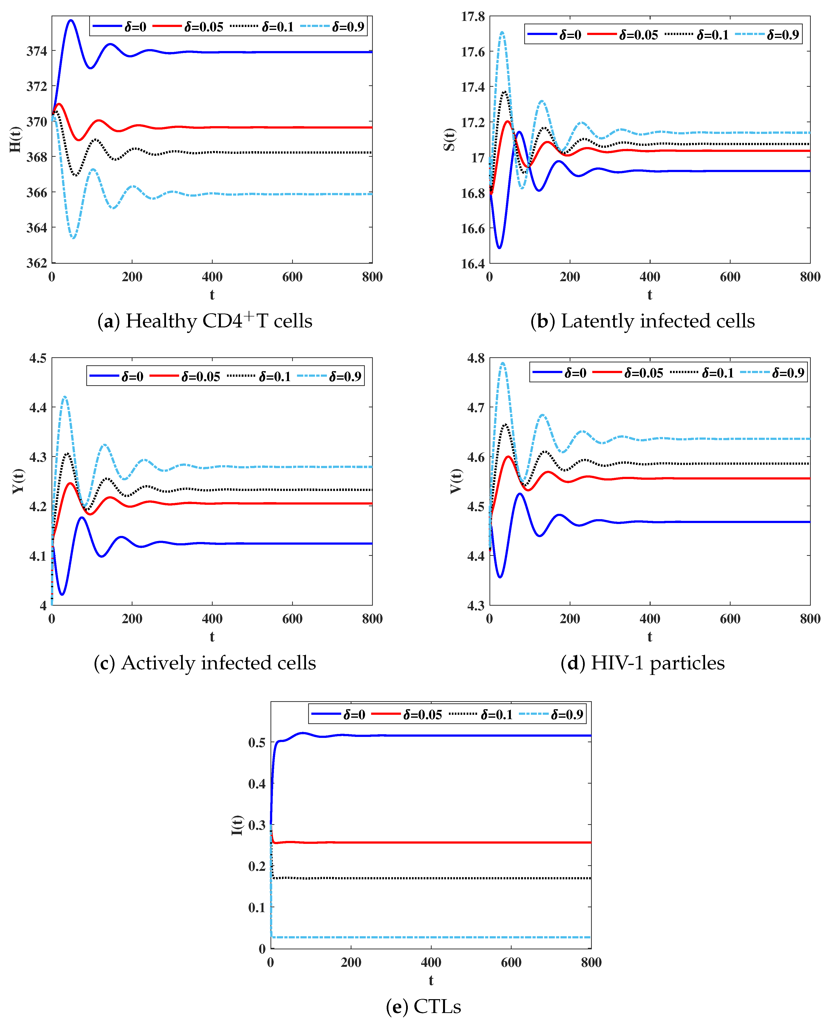
4.1.2. Effect of the CTL Immune Impairment

In this case, we vary the parameter $\delta$ and choose ${\rho }_1=0.003,$ ${\rho }_2=0.0001$ and ${\rho }_3=0.0004.$ To investigate the immune impairment effects on the dynamics of system (8) we solve the system numerically taking under consideration different values of $\delta$ as shown in

Table 2. Effect of the CTL immune impairment parameter.

$\mathit{\delta }$	Equilibria
$\delta =0$	$Q_1=\left(373.8995,16.9216,4.1241,4.4678,0.5155\right)$
$\delta =0.05$	$Q_1=\left(369.6465,17.0366,4.2053,4.5557,0.2563\right)$
$\delta =0.1$	$Q_1=\left(368.2255,17.0750,4.2328,4.5855,0.1698\right)$
$\delta =0.9$	$Q_1=\left(365.8669,17.1387,4.2790,4.6356,0.0264\right)$

. In this case, we select the following initial condition:

IC4:$\left(H\right(0),S(0),Y(0),V(0),I(0\left)\right)=(370,17,4,4.5,0.3)$.

Table 2 shows that as $\delta$ is increased, the concentration of CTLs is decreased. Consequently, the concentration of latently and actively infected cells and free HIV-1 particles are increased. In the mean time, the concentration of healthy CD$4^{+}$T cells is decreased. We observe from Figure 3, that the CTL immune impairment does not change the stability properties of the equilibria, since the parameter ${\Re }_0$ does not depend on $\delta$.

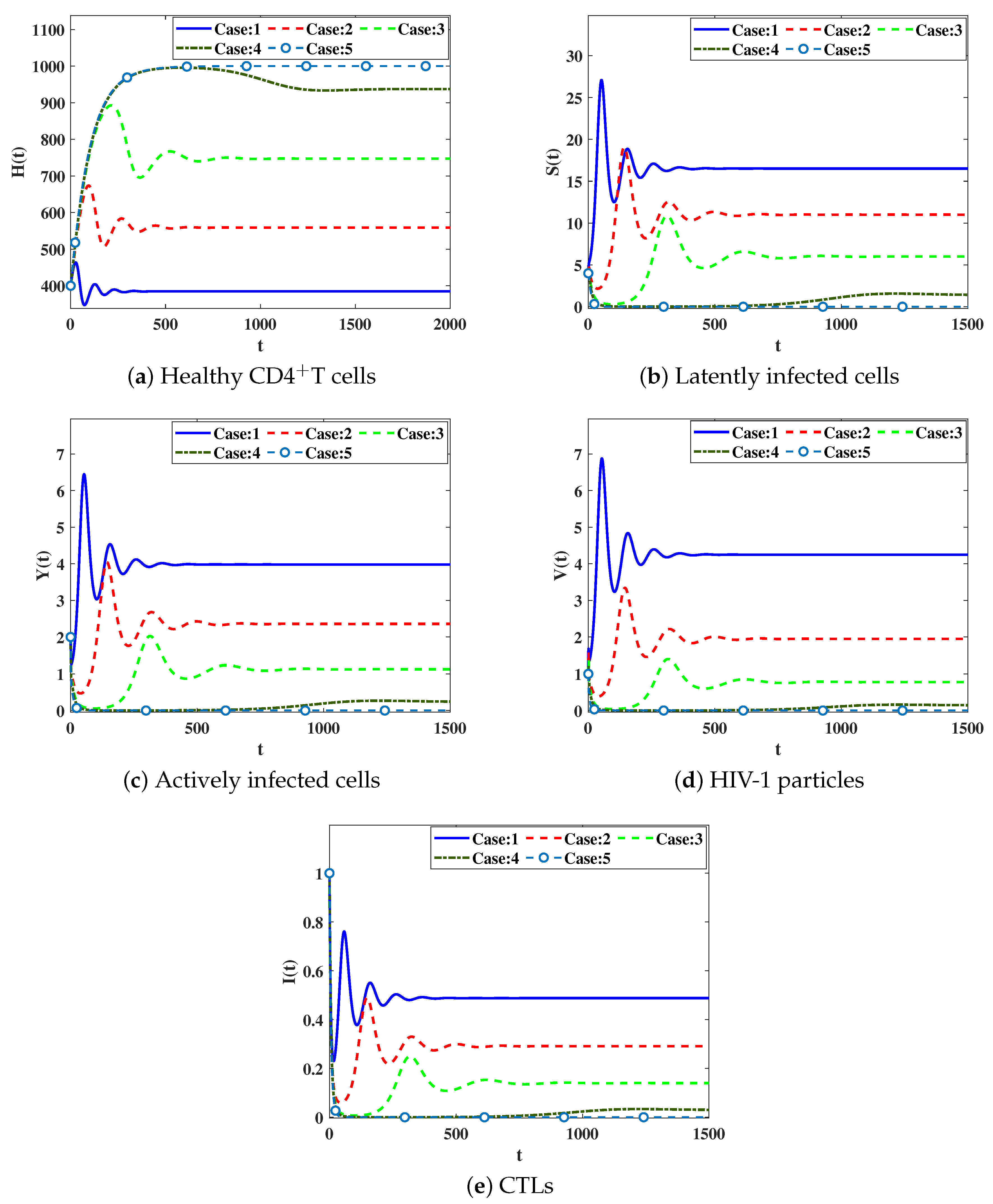
4.2. Numerical Simulation for Model (23)

In this subsection, for numerical purposes, we take a specific form of the probability distributed functions $f_i\left(\varrho \right),$ $i=1,2,3,$ as follows:

$$f_i\left(\varrho \right)={\delta }_{*}\left(\varrho -{\varrho }_i\right),{\varrho }_i\in \left[0,k_i\right],i=1,2,3,$$

where ${\delta }_{*}(.)$ is the Dirac delta function. When $k_i\to \infty ,$ we have

$${\int }_0^{\infty }{f}_i\left(\varrho \right)d\varrho =1,i=1,2,3.$$

Further, we have

$$F_i={\int }_0^{\infty }{\delta }_{*}\left(\varrho -{\varrho }_i\right)e^{-h_i\varrho }d\varrho =e^{-h_i{\varrho }_i},i=1,2,3.$$

Hence, the distributed time delay system (23) will be transformed to a discrete time delay system as:

$$\left\{\begin{array}{cc}\dot{H}\left(t\right)\hfill & =\alpha -\eta H\left(t\right)-{\rho }_{1}H\left(t\right)V\left(t\right)-{\rho }_{2}H\left(t\right)S\left(t\right)-{\rho }_{3}H\left(t\right)Y\left(t\right),\hfill \\ \dot{S}\left(t\right)\hfill & =e^{-h_1{\varrho }_1}H\left(t-{\varrho }_1\right)\left({\rho }_{1}V\left(t-{\varrho }_1\right)+{\rho }_{2}S\left(t-{\varrho }_1\right)\right.\hfill \\ \hfill & \left.+{\rho }_{3}Y\left(t-{\varrho }_1\right)\right)-\left(\sigma +\mu \right)S\left(t\right),\hfill \\ \dot{Y}\left(t\right)\hfill & =\sigma e^{-h_2{\varrho }_2}S\left(t-{\varrho }_2\right)-\tau Y\left(t\right)-\gamma I\left(t\right)Y\left(t\right),\hfill \\ \dot{V}\left(t\right)\hfill & =\epsilon e^{-h_3{\varrho }_3}Y\left(t-{\varrho }_3\right)-\theta V\left(t\right),\hfill \\ \dot{I}\left(t\right)\hfill & =\lambda Y\left(t\right)-\pi I\left(t\right)-\delta I\left(t\right)Y\left(t\right).\hfill \end{array}\right.$$

(38)

For system (38), the basic reproduction number is given as:

$${\tilde{\Re }}_{0\left(38\right)}=\frac{{\tilde{H}}_0{e}^{-h_1{\varrho }_1}\left(\sigma e^{-h_2{\varrho }_2}\left({\rho }_1\epsilon e^{-h_3{\varrho }_3}+{\rho }_3\theta \right)+{\rho }_2\theta \tau \right)}{\left(\sigma +\mu \right)\theta \tau }.$$

(39)

The effect of time delays on stability of equilibria

To investigate the impact of delay parameters on the solutions of system (38), we fix the parameters ${\rho }_1=0.003,$ ${\rho }_2=0.0001,$ ${\rho }_3=0.0004,$ $\delta =0.001,$ $h_1=0.1,$ $h_2=0.2$ and $h_3=0.3.$ On the other hand, the other parameters will be taken from Table 1. Moreover, we vary the delay parameters ${\varrho }_i,$ $i=1,2,3.$ Since ${\tilde{\Re }}_{0\left(38\right)}$ given in Equation (39) depends on ${\varrho }_i$, then changing the parameters ${\varrho }_i$ will change the stability of equilibria. Let us take the following cases of the delay values:

Case: 1 ${\varrho }_1=0.07$, ${\varrho }_2=0.06$, ${\varrho }_3=0.05$.

Case: 2 ${\varrho }_1=0.8$, ${\varrho }_2=0.7$, ${\varrho }_3=0.9$.

Case: 3 ${\varrho }_1=1.3$, ${\varrho }_2=1.4$, ${\varrho }_3=1.5$.

Case: 4 ${\varrho }_1=1.8$, ${\varrho }_2=1.9$, ${\varrho }_3=2$.

Case: 5 ${\varrho }_1=4$, ${\varrho }_2=3$, ${\varrho }_3=5$.

We solve system (38) under initial condition IC5

IC5:$\left(H\right(r),S(r),Y(r),V(r),L(r\left)\right)=(400,4,2,1,1)$, $r\in [-\varrho ,0],$$\varrho =max\{{\varrho }_1,{\varrho }_2,{\varrho }_3\}$. In

Table 3. The disparity of ${\tilde{\Re }}_{0\left(38\right)}$ with respect to the delay parameters.

Delay Parameters $({\mathit{\varrho }}_1,{\mathit{\varrho }}_2,{\mathit{\varrho }}_3)$	Equilibria	${\tilde{\mathit{\Re }}}_{0\left(38\right)}$
$(0.07,0.06,0.05)$	${\tilde{Q}}_{1\left(38\right)}=(384.729,16.513,3.982,4.249,0.488)$	$2.656$
$(0.8,0.7,0.9)$	${\tilde{Q}}_{1\left(38\right)}=(558.891,11.005,2.358,1.95,0.291)$	$1.812$
$(1.3,1.4,1.5)$	${\tilde{Q}}_{1\left(38\right)}=(747.257,5.998,1.125,0.777,0.14)$	$1.346$
$(1.8,1.9,2)$	${\tilde{Q}}_{1\left(38\right)}=(936.985,1.423,0.243,0.144,0.03)$	$1.069$
$(4,3,5)$	${\tilde{Q}}_{0\left(38\right)}=(1000,0,0,0,0)$	$0.461$

, we demonstrate the values of ${\tilde{\Re }}_{0\left(38\right)}$ for different values of ${\varrho }_i,$ $i=1,2,3$. We observe that as the parameters ${\varrho }_i$ are increased, the values of ${\tilde{\Re }}_{0\left(38\right)}$ are decreased. The numerical solutions are displayed in Figure 4. We conclude that a significant effect is caused by the inclusion of time delays which causes increasing in the concentration of healthy CD$4^{+}$T cells and decreasing in the concentrations of latently and actively infected cells, HIV-1 particles and CTL cells.

5. Conclusions and Discussion

In this paper, we introduced two HIV-1 dynamic models with CTL immune impairment. The models consist of five compartments: healthy CD$4^{+}$T cells, latently and actively infected cells, free HIV-1 particles and CTLs. We considered that the healthy CD$4^{+}$T cells become infected by coming into contact with free HIV-1 particles, latently infected cells and actively infected cells. In the second model, we took into account three distributed time delays to be more realistic. We showed that the solutions of the models are nonnegative and bounded. We concluded that each model has two equilibria, the infection-free equilibrium, and the infected equilibrium. We found the basic reproduction number ${\Re }_0$ (or ${\tilde{\Re }}_0$) that controls the existence and global stability of the two equilibria. Number ${\Re }_0$ (or ${\tilde{\Re }}_0$) consists of three parts: the first is the contribution from the VTC infection, the second part is the contribution from the latent CTC spread, and the third part is the contribution from the active CTC spread. For both models, we formulated Lyapunov functions and applied L.I.P to establish the global asymptotic stability of the two equilibria. We proved that if the basic reproduction number ${\Re }_0<1$ (or ${\tilde{\Re }}_0<1$), then the infection-free equilibrium $Q_0$ (or ${\tilde{Q}}_0$) is G.A.S, and thus the infection dies out. Moreover, if ${\Re }_0>1$ (or ${\tilde{\Re }}_0>1$), then $Q_0$ (or ${\tilde{Q}}_0$) is unstable and the infected equilibrium $Q_1$ (or ${\tilde{Q}}_1$) is G.A.S, and thus the infection becomes chronic. Finally, we performed some numerical simulations to illustrate our theoretical results. We showed that the numerical results are consistent with theoretical results

We discussed the effect of immune impairment and time delay on the HIV-1 dynamics. We found that weak immunity contributes significantly to the development of the disease. Moreover, the presence of time delay can significantly decrease the basic reproduction number ${\tilde{\Re }}_0$ and then suppress the HIV-1 replication. Therefore, to eliminate HIV-1 from the body, one should focus on designing control strategies which make ${\tilde{\Re }}_0<1$. Increasing delay parameters ${\varrho }_i$, $i=1,2,3$ may be observed when infected patients are treated with drug therapies against HIV-1.

We note that, when we ignore the latent CTC spread then model (8) leads to model (3)–(7). The basic reproduction number of system (3)–(7) is given by:

$${\widehat{\Re }}_0={\displaystyle \frac{H_0\epsilon \sigma {\rho }_1}{\theta \tau \left(\sigma +\mu \right)}}+{\displaystyle \frac{H_0\sigma {\rho }_3}{\tau \left(\sigma +\mu \right)}}.$$

Clearly, ${\widehat{\Re }}_0<{\Re }_0$, and thus the presence of latent CTC transmission increases the basic reproduction number and then enhances the viral progression. Neglecting the latent CTC spread in the HIV-1 infection model will lead to underestimation of the basic reproduction number. Consequently, the designed drug therapies will not be accurate or sufficient to eradicate the viruses from the body.

Model (8) can be extended by including the diffusion of the cells and viruses as per Refs. [56,57]:

$$\begin{array}{cc}\hfill \frac{\partial H(t,p)}{\partial t}-{\xi }_H\Delta H\left(t,p\right)& =\alpha -\eta H\left(t,p\right)-{\rho }_{1}H\left(t,p\right)V\left(t,p\right)-{\rho }_{2}H\left(t,p\right)S\left(t,p\right)-{\rho }_{3}H\left(t,p\right)Y\left(t,p\right),\hfill \\ \hfill \frac{\partial S\left(t,p\right)}{\partial t}-{\xi }_S\Delta S\left(t,p\right)& ={\int }_0^{k_1}{f}_1\left(\varrho \right)e^{-h_1\varrho }H\left(t-\varrho ,p\right)\left({\rho }_{1}V\left(t-\varrho ,p\right)+{\rho }_{2}S\left(t-\varrho ,p\right)\right.\hfill \\ \hfill & \left.+{\rho }_{3}Y\left(t-\varrho ,p\right)\right)d\varrho -(\sigma +\mu )S\left(t,p\right),\hfill \\ \hfill \frac{\partial Y\left(t,p\right)}{\partial t}-{\xi }_Y\Delta Y\left(t,p\right)& =\sigma {\int }_0^{k_2}{f}_2\left(\varrho \right)e^{-h_2\varrho }S\left(t-\varrho ,p\right)d\varrho -\tau Y\left(t,p\right)-\gamma I\left(t,p\right)Y\left(t,p\right),\hfill \\ \hfill \frac{\partial V\left(t,p\right)}{\partial t}-{\xi }_V\Delta V\left(t,p\right)& =\epsilon {\int }_0^{k_3}{f}_3\left(\varrho \right)e^{-h_3\varrho }Y\left(t-\varrho ,p\right)d\varrho -\theta V\left(t,p\right),\hfill \\ \hfill \frac{\partial I\left(t,p\right)}{\partial t}-{\xi }_I\Delta I\left(t,p\right)& =\lambda Y\left(t,p\right)-\pi I\left(t,p\right)-\delta I\left(t,p\right)Y\left(t,p\right),\hfill \end{array}$$

where p is the position, ${\xi }_w$ is the diffusion coefficient of compartment w and $\Delta =\frac{{\partial }^2}{\partial p^2}$. Some other types of diffusion can also be included in our models (see e.g., [58,59,60]). We leave these points for future work.

References

1. Nowak, M.A.; Bangham, C.R.M. Population dynamics of immune responses to persistent viruses. Science 1996, 272, 74–79. [Google Scholar] [CrossRef]
2. Nowak, M.A.; May, R.M. Virus Dynamics; Oxford University Press: New York, NY, USA, 2000. [Google Scholar]
3. Arnaout, R.; Nowak, M.; Wodarz, D. HIV-1 dynamics revisited: Biphasic decay by cytotoxic lymphocyte killing? Proc. R. Soc. Lond. Ser. Biol. Sci. 1450, 267, 1347–1354. [Google Scholar] [CrossRef] [PubMed]
4. Adak, D.; Bairagi, N. Bifurcation analysis of a multidelayed HIV model in presence of immune response and understanding of in-host viral dynamics. Math. Methods Appl. Sci. 2019, 42, 4256–4272. [Google Scholar] [CrossRef]
5. Li, B.; Chen, Y.; Lu, X.; Liu, S. A delayed HIV-1 model with virus waning term. Math. Biosci. Eng. 2016, 13, 135–157. [Google Scholar] [CrossRef] [PubMed]
6. Wang, K.; Wang, W.; Liu, X. Global Stability in a viral infection model with lytic and nonlytic immune response. Comput. Math. Appl. 2006, 51, 1593–1610. [Google Scholar] [CrossRef]
7. Lv, C.; Huang, L.; Yuan, Z. Global stability for an HIV-1 infection model with Beddington-DeAngelis incidence rate and CTL immune response. Commun. Nonlinear Sci. Numer. Simul. 2014, 19, 121–127. [Google Scholar] [CrossRef]
8. Jiang, C.; Kong, H.; Zhang, G.; Wang, K. Global properties of a virus dynamics model with self-proliferation of CTLs. Math. Appl. Sci. Eng. 2021, 2, 123–133. [Google Scholar] [CrossRef]
9. Jiang, C.; Wang, W. Complete classification of global dynamics of a virus model with immune responses. Discret. Contin. Dyn.-Syst.-Ser. 2014, 19, 1087–1103. [Google Scholar] [CrossRef]
10. Ren, J.; Xu, R.; Li, L. Global stability of an HIV infection model with saturated CTL immune response and intracellular delay. Math. Biosci. Eng. 2020, 18, 57–68. [Google Scholar] [CrossRef]
11. Wang, A.P.; Li, M.Y. Viral dynamics of HIV-1 with CTL immune response. Discret. Contin. Dyn.-Syst.-Ser. 2021, 26, 2257–2272. [Google Scholar] [CrossRef]
12. Yang, Y.; Xu, R. Mathematical analysis of a delayed HIV infection model with saturated CTL immune response and immune impairment. J. Appl. Math. Comput. 2022, 68, 2365–2380. [Google Scholar] [CrossRef]
13. Liu, H.; Zhang, J.-F. Dynamics of two time delays differential equation model to HIV latent infection. Phys. A 2019, 514, 384–395. [Google Scholar] [CrossRef]
14. Perelson, A.; Neumann, A.; Markowitz, M.; Leonard, J.; Ho, D. HIV-1 dynamics in vivo: Virion clearance rate, infected cell life-span, and viral generation time. Science 1996, 271, 1582–1586. [Google Scholar] [CrossRef] [PubMed]
15. Zhu, H.; Zou, X. Dynamics of a HIV-1 infection model with cell-mediated immune response and intracellular delay. Discret. Continuous Dyn.-Syst.-Ser. 2009, 12, 511–524. [Google Scholar] [CrossRef]
16. Shi, X.; Zhou, X.; Song, X. Dynamical behavior of a delay virus dynamics model with CTL immune response. Nonlinear Anal. Real World Appl. 2010, 11, 1795–1809. [Google Scholar] [CrossRef]
17. Li, X.; Fu, S. Global stability of a virus dynamics model with intracellular delay and CTL immune response. Math. Methods Appl. Sci. 2015, 38, 420–430. [Google Scholar] [CrossRef]
18. Shu, H.; Wang, L.; Watmough, J. Global stability of a nonlinear viral infection model with infinitely distributed intracellular delays and CTL immune responses. Siam J. Appl. Math. 2013, 73, 1280–1302. [Google Scholar] [CrossRef]
19. Jolly, C.; Sattentau, Q. Retroviral spread by induction of virological synapses. Traffic 2004, 5, 643–650. [Google Scholar] [CrossRef]
20. Sato, H.; Orenstein, J.; Dimitrov, D.; Martin, M. Cell-to-cell spread of HIV-1 occurs within minutes and may not involve the participation of virus particles. Virology 1992, 186, 712–724. [Google Scholar] [CrossRef] [PubMed]
21. Iwami, S.; Takeuchi, J.S.; Nakaoka, S.; Mammano, F.; Clavel, F.; Inaba, H.; Kobayashi, T.; Misawa, N.; Aihara, K.; Koyanagi, Y.; et al. Cell-to-cell infection by HIV contributes over half of virus infection. eLife 2015, 4, e08150. [Google Scholar] [CrossRef]
22. Komarova, N.L.; Wodarz, D. Virus dynamics in the presence of synaptic transmission. Math. Biosci. 2013, 242, 161–171. [Google Scholar] [CrossRef]
23. Sourisseau, M.; Sol-Foulon, N.; Porrot, F.; Blanchet, F.; Schwartz, O. Inefficient human immunodeficiency virus replication in mobile lymphocytes. J. Virol. 2007, 81, 1000–1012. [Google Scholar] [CrossRef]
24. Sigal, A.; Kim, J.T.; Balazs, A.B.; Dekel, E.; Mayo, A.; Milo, R.; Baltimore, D. Cell-to-cell spread of HIV permits ongoing replication despite antiretroviral therapy. Nature 2011, 477, 95–98. [Google Scholar] [CrossRef] [PubMed]
25. Martin, N.; Sattentau, Q. Cell-to-cell HIV-1 spread and its implications for immune evasion. Curr. Opin. HIV AIDS 2009, 4, 143–149. [Google Scholar] [CrossRef]
26. Guo, T.; Qiu, Z. The effects of CTL immune response on HIV infection model with potent therapy, latently infected cells and cell-to-cell viral transmission. Math. Biosci. Eng. 2019, 16, 6822–6841. [Google Scholar] [CrossRef] [PubMed]
27. Elaiw, A.M.; AlShamrani, N.H. Global stability of a delayed adaptive immunity viral infection with two routes of infection and multi-stages of infected cells. Commun. Nonlinear Sci. Numer. Simul. 2020, 86, 105259. [Google Scholar] [CrossRef]
28. Regoes, R.; Wodarz, D.; Nowak, M.A. Virus dynamics: The effect to target cell limitation and immune responses on virus evolution. J. Theor. Biol. 1998, 191, 451–462. [Google Scholar] [CrossRef] [PubMed]
29. Hu, Z.; Zhang, J.; Wang, H.; Ma, W.; Liao, F. Dynamics analysis of a delayed viral infection model with logistic growth and immune impairment. Appl. Math. Model. 2014, 38, 524–534. [Google Scholar] [CrossRef]
30. Krishnapriya, P.; Pitchaimani, M. Modeling and bifurcation analysis of a viral infection with time delay and immune impairment. Jpn. J. Ind. Appl. Math. 2017, 34, 99–139. [Google Scholar] [CrossRef]
31. Eric, A.V.; Noe, C.C.; Gerardo, G.A. Analysis of a viral infection model with immune impairment, intracellular delay and general non-linear incidence rate. Chaos Solitons Fractals 2014, 69, 1–9. [Google Scholar]
32. Wang, S.; Song, X.; Ge, Z. Dynamics analysis of a delayed viral infection model with immune impairment. Appl. Math. Model. 2011, 35, 4877–4885. [Google Scholar] [CrossRef]
33. Krishnapriya, P.; Pitchaimani, M. Analysis of time delay in viral infection model with immune impairment. J. Appl. Math. Comput. 2017, 55, 421–453. [Google Scholar] [CrossRef]
34. Wang, Z.P.; Liu, X.N. A chronic viral infection model with immune impairment. J. Theor. Biol. 2007, 249, 532–542. [Google Scholar] [CrossRef] [PubMed]
35. Jia, J.; Shi, X. Analysis of a viral infection model with immune impairment and cure rate. J. Nonlinear Sci. Appl. 2016, 9, 3287–3298. [Google Scholar] [CrossRef]
36. Elaiw, A.M.; Raezah, A.A.; Azoz, S.A. Stability of delayed HIV dynamics models with two latent reservoirs and immune impairment. Adv. Differ. Equ. 2018, 50, 1–25. [Google Scholar] [CrossRef]
37. Bai, N.; Xu, R. Mathematical analysis of an HIV model with latent reservoir, delayed CTL immune response and immune impairment. Math. Biosci. Eng. 2021, 18, 1689–1707. [Google Scholar] [CrossRef]
38. Raezah, A.A.; Elaiw, A.M.; Alofi, B.S. Global properties of latent virus dynamics models with immune impairment and two routes of infection. High-Throughput 2019, 8, 16. [Google Scholar] [CrossRef] [PubMed]
39. Alofi, B.S.; Azoz, S.A. Stability of general pathogen dynamic models with two types of infectious transmission with immune impairment. AIMS Math. 2020, 6, 114–140. [Google Scholar] [CrossRef]
40. Zhang, L.; Xu, R. Dynamics analysis of an HIV infection modelwith latent reservoir, delayed CTL immune response and immune impairment. Nonlinear Anal. Model. Control. 2023, 28, 1–19. [Google Scholar] [CrossRef]
41. Elaiw, A.M.; Raezah, A.; Alofi, B.S. Dynamics of delayed pathogen infection models with pathogenic and cellular infections and immune impairment. AIP Adv. 2018, 8, 025323. [Google Scholar] [CrossRef]
42. Agosto, L.; Herring, M.; Mothes, W.; Henderson, A. HIV-1-infected CD4+ T cells facilitate latent infection of resting CD4+ T cells through cell-cell contact. Cell 2018, 24, 2088–2100. [Google Scholar] [CrossRef] [PubMed]
43. Wang, W.; Wang, X.; Guo, K.; Ma, W. Global analysis of a diffusive viral model with cell-to-cell infection and incubation period. Math. Methods Appl. Sci. 2020, 43, 5963–5978. [Google Scholar] [CrossRef]
44. Elaiw, A.M.; AlShamrani, N.H. Stability of a general CTL-mediated immunity HIV infection model with silent infected cell-to-cell spread. Adv. Differ. Equ. 2020, 2020, 355. [Google Scholar] [CrossRef]
45. Alshamrani, N.H. Stability of a general adaptive immunity HIV infection model with silent infected cell-to-cell spread. Chaos Solitons Fractals 2021, 150, 110422. [Google Scholar] [CrossRef]
46. Elaiw, A.M.; AlShamrani, N.H. Stability of a delayed adaptive immunity hiv infection model with silent infected cells and cellular infection. J. Appl. Anal. Comput. 2021, 11, 964–1005. [Google Scholar] [CrossRef]
47. Hattaf, K.; Dutta, H. Modeling the dynamics of viral infections in presence of latently infected cells. Chaos Solitons Fractals 2020, 136, 109916. [Google Scholar] [CrossRef]
48. Elaiw, A.M.; AlShamrani, N.H.; Hobiny, A.D. Stability of an adaptive immunity delayed HIV infection model with active and silent cell-to-cell spread. Math. Biosci. Eng. 2020, 17, 6401–6458. [Google Scholar] [CrossRef] [PubMed]
49. AlShamrani, N.H.; Elaiw, A.M.; Dutta, H. Stability of a delay-distributed HIV infection model with silent infected cell-to-cell spread and CTL-mediated immunity. Eur. Phys. J. Plus 2020, 135, 593. [Google Scholar] [CrossRef]
50. van den Driessche, P.; Watmough, J. Reproduction numbers and sub-threshold endemic equilibria for compartmental models of disease transmission. Math. Biosci. 2002, 180, 29–48. [Google Scholar] [CrossRef]
51. Willems, J.L. Stability Theory of Dynamical Systems; Wiley: New York, NY, USA, 1970. [Google Scholar]
52. Hale, J.K.; Lunel, S.M.V. Introduction to Functional Differential Equations; Springer: New York, NY, USA, 1993. [Google Scholar]
53. Kuang, Y. Delay Differential Equations with Applications in Population Dynamics; Academic Press: San Diego, CA, USA, 1993. [Google Scholar]
54. Sahani, S.K.; Yashi, P. Effects of eclipse phase and delay on the dynamics of HIV infection. J. Biol. Syst. 2018, 26, 421–454. [Google Scholar] [CrossRef]
55. Allali, K.; Danane, J.; Kuang, Y. Global analysis for an HIV infection model with CTL immune response and infected cells in eclipse phase. Appl. Sci. 2017, 7, 861. [Google Scholar] [CrossRef]
56. Elaiw, A.M.; Al Agha, A.D. Analysis of a delayed and diffusive oncolytic M1 virotherapy model with immune response. Nonlinear Anal. Real World Appl. 2020, 55, 103116. [Google Scholar] [CrossRef]
57. Elaiw, A.M.; Al Agha, A.D. Global Stability of a reaction-diffusion Malaria/COVID-19 coinfection dynamics model. Mathematics 2022, 10, 4390. [Google Scholar] [CrossRef]
58. Bellomo, N.; Painter, K.J.; Tao, Y.; Winkler, M. Occurrence vs. Absence of taxis-driven instabilities in a May-Nowak model for virus infection. SIAM J. Appl. Math. 2019, 79, 1990–2010. [Google Scholar] [CrossRef]
59. Ren, X.; Tian, Y.; Liu, L.; Liu, X. A reaction-diffusion within-host HIV model with cell-to-cell transmission. J. Math. Biol. 2018, 76, 831–1872. [Google Scholar] [CrossRef] [PubMed]
60. Bellomo, N.; Outada, N.; Soler, J.; Tao, Y.; Winkler, M. Chemotaxis and cross-diffusion models in complex environments: Models and analytic problems toward a multiscale vision. Math. Model. Methods Appl. Sci. 2022, 32, 713–792. [Google Scholar] [CrossRef]
Figure 1. Solutions of system (8) when 0 < 1 .
Mathematics 11 03743 g001
Figure 2. Solutions of system (8) when 0 > 1 .
Mathematics 11 03743 g002
Figure 3. Solutions of system (8) with different values of the impairment parameter δ .
Mathematics 11 03743 g003
Figure 4. Effect of the delay parameters on the solutions of system (38).
Mathematics 11 03743 g004