A Novel Prediction Model for Seawall Deformation Based on CPSO-WNN-LSTM

Abstract

Admittedly, deformation prediction plays a vital role in ensuring the safety of seawall during its operation period. However, there still is a lack of systematic study of the seawall deformation prediction model currently. Moreover, the absence of the major influencing factor selection is generally widespread in the existing model. To overcome this problem, the Chaotic Particle Swarm Optimization (CPSO) algorithm is introduced to optimize the wavelet neural network (WNN) model, and the CPSO-WNN model is utilized to determine the major influencing factors of seawall deformation. Afterward, on the basis of major influencing factor determination results, the CPSO algorithm is applied to optimize the parameters of Long Short-Term Memory (LSTM). Subsequently, the monitoring datasets are divided into training samples and test samples to construct the prediction model and validate the effectiveness, respectively. Ultimately, the CPSO-WNN-LSTM model is employed to fit and predict the long-term settlement monitoring data series of an actual seawall located in China. The prediction performances of LSTM and BPNN prediction models were introduced to be comparisons to verify the merits of the proposed model. The analysis results indicate that the proposed model takes advantage of practicality, high efficiency, stable capability, and high precision in seawall deformation prediction.

1. Introduction

China boasts a vast coastline stretching over 18,000 km, which provides ample opportunities for the development and utilization of abundant marine resources. However, the coastline generally faces numerous natural disasters. Particularly, an average of 9.5 typhoons per year not only result in windstorms, tidal disasters, and floods in coastal areas but also pose a severe threat to the lives and properties of local residents [1,2]. As a crucial hydraulic structure, seawalls protect the coastline and coastal areas from marine erosion and water hazards by defending against typhoons and tidewater. The structures of seawalls mainly consist of sloping earth embankments, crushed rock revetments, cemented slope embankments, and stone wall embankments. Many existing seawalls are built by renovation and reinforcement of old seawalls in China. A typical cross-section of a current seawall and the old seawall before renovated in China is illustrated in Figure 1; the contour line of the seawall body is marked using a red dotted line. However, accompanied by the frequent erosion caused by tides and typhoons, safety accidents have increased in recent years [3]. In comparison with dams, slopes, or sluices, there is very limited experience in seawall structural behavior analysis due to the complex environment and relatively rare monitoring data. Given the significance of seawalls, their operation states analysis has aroused public awareness for decades.

In the past few years, studies generally focused on the osmosis pressure analysis methods of seawalls and considerable research efforts have been devoted to the osmosis pressure analysis [4,5]. Because deformation is commonly regarded as the most intuitive representation of seawall structural behavior, more attention has been paid to the seawall deformation characteristic analysis. With the rapid development of remote sensing technologies, Synthetic Aperture Radar Interferometry (InSAR) has played an important role in the field of large-scale surface deformation monitoring [6]. Referring to its merits of high monitoring precision, huge space coverage, and high efficiency, InSAR has been implemented extensively in seawall deformation monitoring [7,8,9]. In order to improve the monitoring precision, Qin et al. [10] explored a multi-view InSAR analysis method to realize three-dimensional seawall deformation monitoring. In addition, Unmanned Aerial Vehicle (UAV) lidar has been combined with InSAR to evaluate the safety operation behavior of coastal hydraulic engineering [11].

Recent development of numerical analysis methods provides an additional approach to seawall deformation accurate analysis. Qh et al. [12] simulated the deformation of seawall foundations based on Discontinuous Deformation Analysis (DDA). Kanatani et al. [13] proposed a Distinct Element Method and Finite Element Method (DEM-FEM) coupled analysis method to predict seawall deformation under earthquakes. Jiang et al. [14] employed modified DDA in seawall safety evaluation; the analysis results demonstrated the ancient seawall was generally in a healthy state.

With the aim of discovering the abnormal deformation of seawalls timely, it is vital to forecast the development tendency of seawall deformation characteristics based on historical monitoring data. Therefore, a variety of prediction models of hydraulic structures have been proposed and already applied broadly, which have an obvious advantage over the above methods presented. Qin et al. [15] introduced the Improved Variable Dimension Fraction (IVDF) model and the Artificial Neural Network (ANN) to predict trend item and deviation item of seawall deformation, respectively. Subsequently, Qin et al. [16] established the seawall settlement prediction model based on the least-square (LS) method and the differential self-regression moving average (ARIMA) model. Ma et al. [17] constructed a seawall settlement prediction model based on a back propagation neural network to spot the danger in time. Nevertheless, the deformation of the seawall is owing to the composite effects of many factors; the above model presented suffers a lack of factor importance analysis. This shortcoming could lead to worse robustness of the models due to the effect of multicollinearity among the factors. Therefore, principal component analysis (PCA) [18,19], random forest (RF) [20], linear discriminant analysis (LDA) [21], evidence theory [22], and other algorithms have been introduced to determine important influencing factors of dam deformation. In this case, the overlapping information of factors could be eliminated as much as possible to avoid multicollinearity of factors.

Given that the traditional statistical model, deterministic model, and hybrid model applied in hydraulic structure deformation prediction seem to have difficulty in dealing with multidimensional input, model adaptive learning, and analyzing complicated nonlinear relationships, neural networks have been widely employed to overcome these issues in recent years. On account of the good nonlinear fitting abilities of the multi-layer neural networks, they have been sufficiently utilized in time series prediction. However, conventional multi-layer neural networks usually fail to study and remember long-term dependency information, which limits its application. Hence, the Long Short-Term Memory (LSTM) has been proposed to overcome this shortcoming [23]. Currently, the LSTM neural network has been applied in structural engineering deformation prediction. In contrast to the traditional prediction models, it exhibits excellent prediction performance [24,25].

In summary, in this paper, the possible influencing factors of seawall deformation are analyzed according to the engineering characteristics and surroundings of seawalls primarily. Subsequently, the effects of all influencing factors are analyzed and characterized for prediction model establishment. Considering the obvious advantages in adaptive learning and complicated nonlinear relationship fitting, a wavelet neural network (WNN) is introduced to select major influencing factors of seawall deformation by calculating the importance values. In order to accelerate the convergence speed and improve the calculation efficiency, the Chaotic Particle Swarm Optimization (CPSO) algorithm is used to optimize the parameters of WNN. Therefore, the major influencing factor determination method is presented in Section 2. On the basis of the major factors determined, the seawall deformation prediction model is established based on LSTM in Section 3. The CPSO algorithm is applied to optimize the neural network structures and improve the performance of the LSTM model. The validation of the model is verified using the case study of an actual seawall project located in China in Section 4. The comparison analysis of the prediction results of the models based on RNN, LSTM, and the proposed method is applied to verify the accuracy and comprehensive prediction effects of the proposed method. Finally, the conclusions are drawn in Section 5.

2. Major Influencing Factor Determination Method Based on the CPSO-WNN Model

2.1. The Principle of the WNN

The wavelet neural network (WNN) is proposed by combining wavelet analysis with neural network theory, and its fusion architecture is demonstrated in Figure 2. Figure 2 $\phi \left(a,b,t\right)$ represents the wavelet basis function, a and b denote the extension factor and translation factor of the wavelet basis function $\phi \left(a,b,t\right)$, respectively, t denotes time. $x_i\left(i=1,2,\cdots ,n\right)$ denotes the input variable, n is the number of input layer nodes, $o_k\left(x\right)\left(k=1,2,\cdots ,l\right)$ means the output variable, and l is the number of output layer nodes. The wavelet basic function is adopted as the activation function of the hidden layer nodes [26]. The weights from the input layer to the hidden layer and the thresholds of the hidden layer are replaced using the extension and translation parameters of the wavelet function, respectively.

In the process of major factor determination, all the monitoring data of influencing factors such as water level, wind speed, and rainfall that influence the variation of seawall deformation monitoring data are treated as one-dimensional signal s(t) and fed into the network. The corresponding wavelet basis function $\phi (a,b,t)$ for the network can be represented as follows:

$$\phi (a,b,t)=\frac{1}{\sqrt{\left|a\right|}}{\phi }_b\left(\frac{t-b}{a}\right)$$

(1)

where ${\phi }_b\left(t\right)$ represents the basis wavelet or mother wavelet; $1/\sqrt{\left|a\right|}$ is the normalized coefficient.

All the input data of the influencing factors $s\left(t\right)$ could be fitted by using the wavelet basis function $\phi \left(a,b,t\right)$, and the fitted data $\widehat{s}\left(t\right)$ of the seawall deformation monitoring data considering the influence of all factors can be expressed as:

$$\hat{s}(t)={\displaystyle \sum _{k=1}^K{w}_k}\phi \left(\frac{t-b_k}{a_k}\right)$$

(2)

where K represents the number of wavelet bases; $w_k$ represents the weight.

The corresponding energy function of $\hat{s}\left(t\right)$ can be written as:

$$E=\frac{1}{2}{\displaystyle \sum _{t=1}^{T_s}{[s(t)-\widehat{s}(t)]}^2}$$

(3)

where E is the value of the energy function of the wavelet neural network, which describes the fitting performance of the network; T_s represents the total time. Equation (3) is also referred to as the error function.

Assuming that the input vector of the influencing factors is $X={(x_1,x_2,\cdots ,x_n)}^T$, the hidden layer vector is $\Psi ={({\phi }_1,{\phi }_2,\cdots ,{\phi }_m)}^T$, and the output vector is the seawall deformation monitoring data $O={(o_1,o_2,\cdots ,o_l)}^T$. Subsequently, the WNN model for the major influencing factors determination of seawall deformation can be established with the n-m-p network structure. In this model, the extension factor vector and translation factor vector are denoted as $a={(a_1,a_2,\cdots ,a_m)}^T$ and $b={(b_1,b_2,\cdots ,b_m)}^T$, respectively. The weight matrix between the hidden layer and the output layer is represented as $W_{m\times l}$.

The analysis process of the WNN model for the major factors determination is generally categorized into forward propagation of the input data and backward propagation of the errors. Supposing that the output vector of the desired target is $D={(d_1,d_2,\cdots ,d_l)}^T$, the principle of the major factor influencing factor determination of the seawall deformation based on WNN is studied below.

(1) In the forward propagation process, the data of the factors influencing are fitted using the wavelet basis function $\phi (a,b,t)$. After weighted computation and passing through the hidden layer, the output data of the seawall deformation can be obtained. The activation function $f(x)$ of the output layer is given by:

$$f(x)=\frac{1}{1+e^{-x}}$$

(4)

The input data of the influencing factor of the j-th neuron in the hidden layer is:

$$ne{t}_j={\displaystyle \sum _{i=1}^n{w}_{ij}{x}_i}$$

(5)

where w_ij denotes the weight from the i-th neuron in the input layer to the j-th neuron in the hidden layer.

After being activated using the wavelet function, it becomes:

$$y_j=\phi (\frac{ne{t}_j-b_j}{a_j})=\phi (\frac{{\displaystyle \sum _{i=1}^n{x}_i}-b_j}{a_j})$$

(6)

Then, the input data of the k-th neuron in the output layer by the weighted computation is:

$$ne{t}_k^{\prime }={\displaystyle \sum _{j=1}^m{w}_{jk}{y}_j=}{\displaystyle \sum _{j=1}^m{w}_{jk}\phi (\frac{{\displaystyle \sum _{i=1}^n{x}_i-b_j}}{a_j})}$$

(7)

With the activation of the function $f(x)$, the output data of the k-th neuron in the output layer for seawall deformation can be expresses as:

$$o_k=f(ne{t}_k)=f\left[{\displaystyle \sum _{j=1}^m{w}_{jk}\phi (\frac{{\displaystyle \sum _{i=1}^n{x}_i-b_j}}{a_j})}\right]$$

(8)

The corresponding forward propagation error function is:

$$\begin{array}{l}E=\frac{1}{2}{\displaystyle \sum _{k=1}^l{(d_k-o_k)}^2}\\ =\frac{1}{2}{{\displaystyle \sum _k^l\left(d_k-f\left({\displaystyle \sum _{j=1}^m{w}_{jk}\phi (\frac{{\displaystyle \sum _{i=1}^n{x}_i-b_j}}{a_j})}\right)\right)}}^2\end{array}$$

(9)

where $o_k$ represents the k-th output data of the seawall deformation; d_k represents the k-the measured data of the seawall deformation; w_jk represents the weight from the j-th neuron in the hidden layer to the k-th neuron in the output layer; a_j and b_j are the wavelet extension and translation factors of the j-th neuron in the hidden layer, respectively.

(2) Backward propagation of the errors occurs when the error function value E of the influencing factors cannot satisfy the set error limit e. The weight w_jk, the extension factor a_j, and the translation factor b_j all need to be adjusted. The adjustment formulas for the above parameters can be determined by:

$$\left\{\begin{array}{l}{w}_{jk}(t+1)=w_{jk}(t)+\mathrm{\Delta }{w}_{jk}\\ a_j(t+1)=a_j(t)+\mathrm{\Delta }{a}_j\\ b_j(t+1)=b_j(t)+\mathrm{\Delta }{b}_j\end{array}\right.$$

(10)

where t denotes the iteration number; $\mathrm{\Delta }{w}_{jk}$ represents the adjustment increment of the weight; $\mathrm{\Delta }{a}_k$ is the adjustment increment of the extension factor; $\mathrm{\Delta }{b}_k$ is the adjustment increment of the translation factor.

Checking whether the error E satisfies the set error limit after each iteration plays a vital role in the process of major influencing factor determination. If it satisfies the condition, the values of the desired parameters (weights, translation factors, and extension factors) are output. If it does not satisfy the condition, the calculation is performed again following the previous steps.

2.2. Parameter Optimization Method for WNN Based on CPSO

Due to the complex influencing factors of seawall deformation, the number of factors input to the WNN model and the number of hidden layer nodes of WNN are also numerous. Therefore, the computing time decreases when calculating the weights, extension factors, and translation factors by employing conventional iterative methods. Deceased convergence speed of the major influencing factor determination and local optimal problem easily occur as the dimensionality of the input factors increases [27,28]. To avoid these problems, the CPSO algorithm is introduced to improve the efficiency of the convergence computation speed of WNN.

CPSO is developed from the traditional Particle Swarm Optimization (PSO) algorithm. PSO treats the values of the parameters (weights, extension factors, and translation factors) in the WNN model as the position coordinates of particles in a D-dimensional space. D is the total number of parameters in the WNN model. The particle position coordinate vector is denoted as X. The particle velocity vector is denoted as V, which corresponds to the adjustment increments of the parameters. Each particle also has a fitness value E, which represents the error between the measured data and the output values of WNN. When PSO is performed to optimize the parameters of the WNN model, the forward propagation process of WNN remains unchanged. In the backward propagation process, the position and velocity of the i-th particle are $X_i=(x_1,x_2,\cdots ,x_D)$ and $V_i=(v_1,v_2,\cdots ,v_D)$, respectively. The particle’s velocity is adjusted, and the particle’s position is updated based on the local best value and global best value. Meanwhile, the fitness value E is calculated. On this basis, the error backpropagation process can be realized as written in Equation (10). Figure 3 illustrates this process, $v_{id}^{t+1}$represents the d-dimensional component of the velocity vector of the i-th particle at the t + 1-th iteration, $v_{id}^t$ denotes the d-dimensional component of the velocity vector of the i-th particle at the t-th iteration, $x_{id}^t$ represents the d-th component of the i-th position of the t-th iteration vector, $o_{id}$ represents the d-th component of the i-th particle at best historical position, $o_{gd}$ is the d-th component of the global best position of the i-th particle, o_i is the historically optimal position, and o_g is the global optimal position.

The calculation formulas are given by:

$$v_{id}^{t+1}=v_{id}^t+c_1(o_{id}-x_{id}^t)+c_2(o_{gd}-x_{id}^t)$$

(11)

$$x_{id}^{t+1}=x_{id}^t+v_{id}^{t+1}$$

(12)

In Equations (11) and (12), c₁ and c₂ are learning factors whose values are typically chosen from the range [0, 2].

Collectively, it can be observed that the initial positions of particles and the velocity update algorithm are of great significance to the convergence of the WNN model. Given the good randomness and exploratory characteristics of the chaos method [29], chaos chaotic properties are applied in the PSO to enhance the optimization effects of the WNN model.

Chaos can be regarded as a type of nonlinear phenomenon that refers to the random-like motion generated using deterministic equations. For example, the Logistic map is a typical chaotic system, and its iterative formula can be defined as:

$$z_{t+1}=\mu z_t(1-z_t)$$

(13)

where $\mu$ is the control parameter, when $\mu =4$ and the initial value z₀ within the range of [0, 1], the output data z of the Logistic map exhibits chaotic characteristics.

By mining process of the main influencing factors of the monitoring effect quantities in seawalls, the basic idea is to confer chaotic characteristics onto the distribution and trend of particle positions. Specifically, the chaotic optimization consists of the following two parts:

(1) The initial positions and velocities of particles are generally random. The exploratory nature of chaos is utilized to generate a large number of initial populations. Then, the dominant populations are selected from them to improve the efficiency of major influencing factor determination. The optimization process of CPSO is simplified to a D-dimensional optimization problem, which can be described as:

$$\min f(x_1,x_2,\cdots ,x_D)s.t.a_d\le x_d\le b_d$$

(14)

where s.t. is the abbreviation of “subject to”, which means the constraint condition.

First, a D-dimensional vector $z^0=[z_{01},z_{02},\cdots ,z_{0D}]$ is randomly generated, and each element value of $z^0$ are randomly selected from [0, 1]. A logistic map of $\mu =4$ is used as the chaotic signal source, and z⁰ is substituted into Equation (14) to obtain $z^1=[z_{11},z_{12},\cdots ,z_{1D}]$ and calculated z² by z¹. The iterative formulas for calculating the element z_j+1,_d in z^j+1 by the element z_jd in z^j are given by:

$$z_{j+1,d}=\mu z_{jd}(1-z_{jd})$$

(15)

where $d=1,2,\cdots ,D$; j represents the iteration number.

For N particles, assuming that the total number of iterations is N, and $z^1~z^N$is calculated. The chaotic factor matrix Z for the major influencing factors determination of the seawall deformation can be defined as:

$$Z={(z^1,z^2,\cdots ,z^N)}^T=\left(\begin{array}{ccc}{z}_{11}& \dots & z_{1D}\\ ⋮& \ddots & ⋮\\ z_{N1}& \cdots & z_{ND}\end{array}\right)$$

(16)

where the element Z_id of Z represents the initial value range $[a_d,b_d]$ of the d-th dimension for the i-th particle, the initial value $x_{id}$ with chaotic characteristics can be expressed as:

$$x_{id}=a_d+(b_d-a_d)z_{id}$$

(17)

On this basis, the seawall deformation error values of N particles are calculated by introducing the objective function. Among them, m particles with better performance are selected as the initial population for further computations.

(2) In Equation (15), the velocity update method refers to both individual and group information of the particles. When the determination process of the major influencing factors gradually converges, it is easy to fall into local optimum. Therefore, perturbations and suppressions are generated in the particles to improve their ability to escape local optima by means of the sensitivity and randomness of chaos. A suppression factor $\gamma$ is introduced into the algorithm, and the direction of particle movement is determined by taking the value of $\gamma$ as 1 or −1. The chaotic factor $\mathrm{\Delta }{x}_{id}$ is established for each velocity component; the impact on the velocity $v_{id}^{t+1}$ can be obtained by:

$$v_{id}^{t+1}=\omega v_{id}^t+{\gamma }_i[c_1(o_{id}-x_{id}^t)+c_2(o_{gd}-x_{id}^t)]+c_3\mathrm{\Delta }{x}_{id}$$

(18)

where $\mathrm{\Delta }{x}_{id}$ represents the chaotic factor; $c_3$ denotes the coefficient of the chaotic factor $\mathrm{\Delta }{x}_{id}$, which is applied to adjust the magnitude of $\mathrm{\Delta }{x}_{id}$.

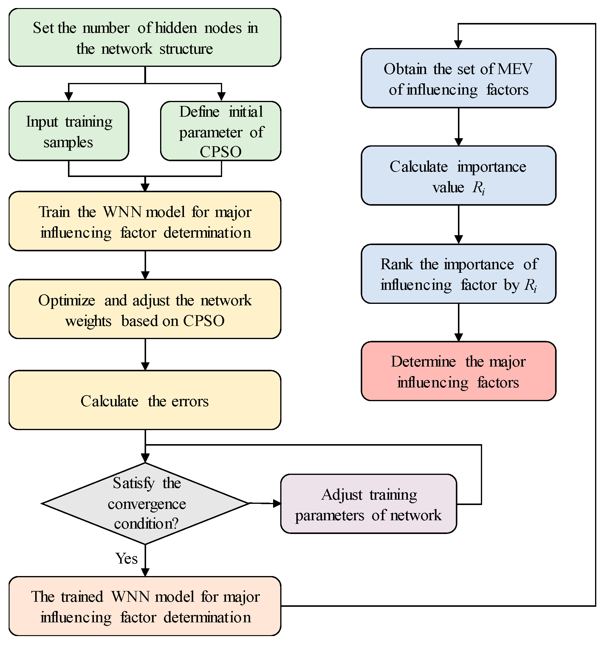
2.3. The Principle of Major Influencing Factor Determination Based on CPSO-WNN Model

The basic idea of the major influencing factor determination based on the CPSO-WNN model is to identify the important factors that affect seawall deformation while discarding the insignificant factors. In the trained WNN model, the various influencing factors correspond to the input neurons of the network, and the deformation values correspond to the output neurons. The key step that affects the efficiency of the CPSO-WNN model is to determine the influence degree of the input neurons’ data on the output neurons’ data. To reflect the importance of each factor’s impact on seawall deformation, the research on the measurement method for the degree of the input data influence on the output data is carried out. The Mean Effect Value (MEV) is adopted to be the evaluation indicator, which can be engaged to reflect the influence degree of the factors on seawall deformation. The calculation principle of MEV is illustrated as follows.

After training the WNN model net based on CPSO, the training samples $X=\left\{x_1,x_2,\cdots ,x_n\right\}$ of the effect of influencing factors are input. Two new training sample datasets $X^{(1)}$ and $X^{(2)}$ are created by increasing and decreasing the original values by 10%, respectively. Subsequently, the data $x_i^{(1)}$ and $x_i^{(2)}$ of the i-th input neuron of $X^{(1)}$ and $X^{(2)}$ are selected, which are combined with the original values of other input neurons to construct input data. The output results $O^{(1)}$ and $O^{(2)}$ are obtained by the trained WNN model, and the output data of the k-th output neuron is represented as follows:

$$o_k^{(1)}=f\left(ne{t}_k\right)=f\left[{\displaystyle \sum _{j=1}^m{w}_{jk}}\phi (\frac{{\displaystyle \sum _{i=1}^n{x}_i^{(1)}}-b_j}{a_j})\right]$$

(19)

$$o_k^{(2)}=f\left(ne{t}_k\right)=f\left[{\displaystyle \sum _{j=1}^m{w}_{jk}}\phi (\frac{{\displaystyle \sum _{i=1}^n{x}_i^{(2)}}-b_j}{a_j})\right]$$

(20)

The difference calculated between $o_k^{(1)}$ and $o_k^{(2)}$ can be regarded as the influence of the influencing factor on the output deformation of the k-th output neuron; the Effect Value (EV) of l output deformation data can be denoted as:

$$\mathrm{\Delta }{O}_i={\displaystyle \sum _{k=1}^l\left(\left|o_k^{(1)}-o_k^{(2)}\right|\right)}$$

(21)

On the basis of the impact values obtained, the MEV of the influencing factors is calculated by taking the average of $\mathrm{\Delta }{O}_i$ according to the monitoring frequency p of the deformation data. The calculation formula of MEV can be expressed as:

$$\mathrm{\Delta }{\overline{O}}_i=\frac{\mathrm{\Delta }{O}_i}{p}=\frac{{\displaystyle \sum _{k=1}^l\left(\left|o_k^{(1)}-o_k^{(2)}\right|\right)}}{p}$$

(22)

Following the above steps, MEV is calculated for each influencing factor of the corresponding input neurons of the WNN model under independent variation conditions. The values of MEV are ranked to analyze the importance of each influencing factor. For the n input factors of the WNN model, there is:

$$\mathrm{\Delta }{\overline{O}}_1\le \mathrm{\Delta }{\overline{O}}_2\le \dots \le \mathrm{\Delta }{\overline{O}}_n$$

(23)

where $\mathrm{\Delta }{\overline{O}}_n$ denotes the influence factor, which is relatively important to seawall deformation.

In this paper, each component of seawall deformation that represents the effect of each influencing factor can be considered as an input factor of the WNN model. Furthermore, the number of hidden layer neurons m of the model plays a vital role in the convergence of the major influencing factor identification. A larger value of m results in more accurate analysis results. However, it will also lead to an increase in the computation time. Therefore, m can be determined properly by an empirical formula [30]:

$$m=\sqrt{n+l}+l$$

(24)

where n is the number of neurons in the WNN model for input data of influencing factors; l is the number of neurons in the WNN model for output data of seawall deformation, and l is usually a constant term, $l\le 20$.

Once the input factors and network node numbers are determined, the structure of the WNN model becomes $n-m-l$. The number of extension factors a and translation factors b is equal to the number of hidden layer neurons m. The number of weights in the WNN model is $m\ast l$, and thus, the total number of unknown parameters that need to be computed for the WNN model is D, which can be calculated by:

$$D=m\ast l+m+m$$

(25)

After optimizing the parameters of the WNN model based on CPSO, the influence of the variations of the input factor data on the output neuron data of the deformation monitoring data is calculated. The MEV values’ set $\left\{\mathrm{\Delta }{\overline{O}}_1,\mathrm{\Delta }{\overline{O}}_2,\cdots ,\mathrm{\Delta }{\overline{O}}_n\right\}$ are constructed, and the elements within the set are normalized. The normalized importance values of the influencing factors are determined. The normalized importance value R_i for the i-th influencing factor of seawall deformation can be expressed as:

$$R_i=\frac{\mathrm{\Delta }{\overline{O}}_i}{{\displaystyle \sum _{j=1}^n\mathrm{\Delta }{\overline{O}}_j}},i=1,2,\cdots ,n$$

(26)

According to the importance values of the various influencing factors, the major influencing factors of seawall deformation can be determined finally, and the whole procedure based on CPSO-WNN is illustrated in Figure 4.

3. CPSO-WNN-LSTM Prediction Model for Seawall Deformation

In this section, we will introduce the LSTM neural network to establish the seawall deformation prediction model.

3.1. Analysis of Each Component of Seawall Deformation

The seawall deformation can be commonly categorized into two types: vertical deformation (i.e., settlement) and horizontal deformation. Then, we analyze the effects of various influencing factors, which compose the components of seawall deformation.

3.1.1. Component of Seawall Settlement

Water pressure, temperature, time effect, wind speed, and tide contribute a lot to the seawall deformation variation; their influences are regarded as every seawall deformation component.

(1)

Water pressure component

Water pressure can be decomposed into horizontal force and vertical force. The vertical force leads to vertical deformation of the seawall, while the submerged part below the waterline is affected by buoyancy, resulting in an upward load on the seawall and reducing the vertical deformation. Above all, the expression for the water pressure component at one monitoring time can be determined as follows:

$${\delta }_{H_1}={\displaystyle \sum _{i=0}^3{a}_{1i}{H}^i}$$

(27)

where H denotes the water depth at one monitoring time; a_1i is the regression coefficient.

(2)

Water level variation lagging effect component

The influence of water level variation on settlement always exhibits a lagging effect, which can be expressed in two ways.

① Average water depth in the early stage. The lagging effect can be represented by the average water depth in the early stage as follows:

$${\delta }_{H_2}={\displaystyle \sum _{i=1}^{m_1}{a}_{2i}}{\overline{H}}_i$$

(28)

where ${\overline{H}}_i$ represents the average water depth over the previous n hours at the monitoring time, i = 1,2,5,10,15,…,m₁; a_2i denotes the regression coefficient.

② Equivalent water depth. To account for the lagging effect of water level changes on settlement, it is necessary to explore the quantification method for the equivalent water depth. Since the influence process of water level variation on settlement approximately follows a normal distribution, the water pressure component can be represented as:

$${\delta }_{H_2}=a_1{\displaystyle {\int }_{-\infty }^0\frac{1}{\sqrt{2\pi }{x}_2}{\mathrm{e}}^{\frac{-{(t-x_1)}^2}{2x_2^2}}{H}_i(t)}dt=a_1{H}_m$$

(29)

where $H_i(t)$ is the water depth at time t; $H_m$ is the equivalent water depth; x₁ is the lagging time of water pressure, which is counted by hours; x₂ is the standard deviation of the normal distribution for water pressure variation, which is the influence time; a₁ is the regression coefficient.

The values of x₁ and x₂ need to be determined using trial calculations to obtain the actual lagging time, thus improving the regression accuracy. To transfer the continuous integration into discrete integration, the integration interval could be taken as 2 to 3 times the value of x₂.

For computational convenience, we adopt the average water depth in the previous period to represent the lagging effect of water level variation. Hence, the water pressure component ${\delta }_H$ is given by:

$${\delta }_H={\displaystyle \sum _{i=0}^3{a}_{1i}{H}^i}+{\displaystyle \sum _{i=1}^{m_1}{a}_{2i}}{\overline{H}}_i$$

(30)

(3)

Temperature component

In mild regions, the seawall deformation is slightly susceptible to temperature. Conversely, in cold regions, freeze–thaw action contributes a lot to the seawall deformation. Therefore, the impact of temperature on seawall deformation is taken into full consideration. In the absence of actual temperature data for the seawall, the multi-period harmonic is selected as the factor, which can be obtained by:

$${\delta }_T=f(T_0,T_0<0 °\mathrm{C}){\displaystyle \sum _{i=1}^{m_2}\left(b_{1i}\sin \frac{2\pi it}{L}+b_{2i}\cos \frac{2\pi it}{L}\right)}$$

(31)

where when i = 1, it means a full period; when i = 2, it is a half-period; m₂ can be typically taken as 1 or 2; $b_{1i}$ and $b_{2i}$ are coefficients; t is the cumulative hours from the monitoring time to the initial monitoring time; $f(T_0,T_0<0 °\mathrm{C})$ is the switching function; T₀ is the air temperature; L represents the length of the freeze–thaw period.

(4)

Time effect component

The seawall settlement caused by the time effect is mainly due to the consolidation of the soil. According to the consolidation theory, the settlement process is essentially the gradual dissipation of pore water in the soil, leading to a reduction in pore volume, as well as the gradual transfer and adjustment of stresses between the soil framework and pore water.

Assuming that in the soil of a width of 2l, the pore water pressure at each point is p, and the total pore water pressure U is given by:

$$U={\displaystyle {\int }_0^{2l}pdx=}{\displaystyle {\int }_0^{2l}\frac{4\sigma }{\pi }{\displaystyle \sum _{i=1,3,5\dots }^{\infty }\frac{1}{i}}\sin \frac{\pi ix}{2l}{e}^{-i^{2}m\theta }dx}$$

(32)

For a saturated soil layer, the consolidation settlement is expressed as follows:

$${\delta }_{\theta }=\frac{2\sigma l-U}{2\sigma l}=1-\frac{8}{{\pi }^2}(e^{-m\theta }+\frac{1}{9}{e}^{-9m\theta }+\dots )$$

(33)

where $\sigma$ represents the consolidation settlement; $m=\frac{{\pi }^{2}C}{4l^2}$; $C=\frac{K(1+{\epsilon }_0)}{\alpha {\gamma }_{\omega }}$; K is the coefficient of permeability; ${\epsilon }_0$ is the initial void ratio before compression; $\alpha$ is the compression index; ${\gamma }_{\omega }$ is the water unit weight.

In Equation (33), the series within the brackets converges rapidly, and it is assumed that the first term provides sufficient accuracy, thus simplifying the consolidation settlement ${\delta }_{{\theta }_1}$ to:

$${\delta }_{{\theta }_1}=1-\frac{8}{{\pi }^2}{e}^{-m\theta }$$

(34)

From Equation (34), it is evident that ${\delta }_{\theta }$ attenuates with time. If the settlement caused by the creep behavior of the soil is considered, the expression for the time effect component ${\delta }_{\theta }$ is as follows:

$${\delta }_{\theta }=c_1\theta +c_2\ln \theta$$

(35)

where $\theta$ represents the cumulative time divided by 100; c₁, c₂ are coefficients.

(5)

Wind speed component:

Frequent and extreme weather events often appear in coastal regions, which come with high winds. Therefore, the effect of wind speed on the settlement variation of the seawall needs to be considered, and the wind speed component ${\delta }_v$ is given by:

$${\delta }_v={\displaystyle \sum _i^{m_3}{f}_i}{V}^i$$

(36)

where m₃ is generally taken as 1 to 3; f_i is a coefficient; V represents the wind speed at the monitoring time.

(6)

Tide component:

Seawall deformation monitoring data reveal distinct periodicity; moreover, tides exhibit a regular rise and fall pattern. Hence, the influence of tidal factors needs to be considered. Assuming a tidal period of one hour, the tidal component ${\delta }_t$ can be expressed as follows:

$${\delta }_t=k_1\cos \left(\frac{2\pi t}{24}\right)+k_2\sin \left(\frac{2\pi t}{24}\right)$$

(37)

where k₁ and k₂ are coefficients; t represents the cumulative hours from the monitoring time to the initial monitoring time.

Above all, the seawall settlement variation can be expressed as:

$$\begin{array}{ll}\delta & =a_0+{\displaystyle \sum _{i=0}^3{a}_{1i}{H}^i}+{\displaystyle \sum _{i=1}^{m_1}{a}_{2i}}{\overline{H}}_i+{\displaystyle \sum _i^{m_3}{f}_i}{V}^i+c_1\theta +c_2\ln \theta \\ & +f(T_0,T_0<0 °\mathrm{C}){\displaystyle \sum _{i=1}^{m_2}\left(b_{1i}\sin \frac{2\pi it}{L}+b_{2i}\cos \frac{2\pi it}{L}\right)}+k_1\cos \left(\frac{2\pi t}{24}\right)+k_2\sin \left(\frac{2\pi t}{24}\right)\end{array}$$

(38)

where a₀ is the constant term, and the meanings of other parameters are the same as previously defined.

3.1.2. Component of Seawall Horizontal Deformation

During the operational period, the seawall occurs horizontal deformation due to the horizontal force of water pressure or seepage forces. Simultaneously, during the consolidation and secondary consolidation processes of the soil, lateral expansion will lead to horizontal deformation along with settlement. Therefore, the horizontal deformation is also influenced by water pressure, temperature, time effect, wind speed, and tides; the expression of seawall horizontal deformation is the same as in Equation (38).

3.2. Seawall Deformation Prediction Model Construction Method Based on CPSO-WNN-LSTM

3.2.1. Long Short-Term Memory Neural Network

Long Short-Term Memory Neural Network (LSTM) is an improved neural network architecture based on Recurrent Neural Network (RNN). RNN generally consists of input, hidden, and output layers. X_t means the feature vector inputted into RNN, U is the parameter matrix from the input layer to the hidden layer, A_t denotes the vector in the hidden layer, W signifies the weight matrix at each time step, V represents the parameter matrix from the hidden layer to the output layer, and Y_t is the feature vector outputted from RNN. The updated formulas of Y_t and X_t are:

$$Y_t=g\left(V\cdot A_t\right)$$

(39)

$$A_t=f\left(U\cdot X_t+W\cdot A_{t-1}\right)$$

(40)

Nevertheless, there seems to be a forgetting condition appearing in RNN as processing long-term information. To overcome this problem, LSTM has been proposed, which incorporates a “forget gate” to enhance the network’s architecture. LSTM introduces cell state and gate mechanisms in the hidden layer calculations, which sets each hidden unit in RNN as a memory cell to remember long-term information. LSTM is composed of the forget gate, the input gate, and the output gate.

The forget gate reads the previous hidden state h_t−1 at the last time and the current data x_t, then regulates the proportion of the previous cell state C_t−1 transferred to the current cell state C_t. The input gate is responsible for controlling the proportion of the current network input X_t transferred to the current cell state C_t. The output gate regulates the proportion of the current cell state C_t transferred to the current output value h_t. The update formulas for the above gates are illustrated as follows:

Door control unit:

$$f_t=\sigma \left(W_f\cdot [h_{t-1},x_t]+b_f\right)$$

(41)

$$i_t=\sigma \left(W_i\cdot \left[h_{t-1},x_t\right]+b_i\right)$$

(42)

$$o_t=\sigma \left(W_o\cdot \left[h_{t-1},x_t\right]+b_o\right)$$

(43)

Memory cell:

$$\widetilde{C_t}=\tanh \left(W_C\cdot \left[h_{t-1},x_t\right]+b_C\right)$$

(44)

Output State:

$$Y_t=o_t\ast \tanh \left(C_t\right)$$

(45)

where W represents the weight of the input variable; b denotes the bias vector; $\sigma$ is the sigmoid activation function, mapping the real number to [0, 1].

The usage of memory cells and control gates of LSTM enables the model to retain information from earlier time steps and capture long-range dependencies in long-term sequential data. Furthermore, the cell state is able to prevent the vanishing gradient problem. The structure of LSTM is depicted in Figure 5.

3.2.2. The Construction Process of Prediction Model Based on CPSO-WNN-LSTM

With the aim of improving the prediction ability and precision of LSTM, the CPSO presented in Section 2.2 can be utilized to optimize the parameters of LSTM. Additionally, the construction process of the seawall deformation prediction model is illustrated as follows. The flowchart of the prediction model construction process is exhibited in Figure 6.

(1) Determine major influencing factors of seawall deformation on the basis of the CPSO-WNN model and generate the training samples and test samples of deformation components caused by major influencing factors.

(2) Generate the training samples and test samples of seawall deformation.

(3) Establish the objective function f of parameter optimization of LSTM, and then optimize the parameters of LSTM by CPSO.

$$f=\sqrt{\frac{{\displaystyle {\sum }_{i=1}^N{\left({\widehat{\delta }}_i-{\delta }_i\right)}^2}}{N}}$$

(46)

where ${\widehat{\delta }}_i$ denotes the deformation calculated value by the model; ${\delta }_i$ represents the deformation monitoring data; N is the number of the data.

(4) Verify the prediction effect of the CPSO-WNN-LSTM model according to test samples of seawall deformation components. The coefficient of determination R² based on the training samples and the root mean square error (RMSE) of test samples is applied to verify the prediction effect.

$$R=\frac{{\displaystyle {\sum }_{i=1}^N{\left({\widehat{\delta }}_i-\overline{\delta }\right)}^2}}{{\displaystyle {\sum }_{i=1}^N{\left({\delta }_i-\overline{\delta }\right)}^2}}$$

(47)

$$RMSE=\sqrt{\frac{1}{M}{\displaystyle \sum _{j=1}^M{\left({\delta }_j-{\widehat{\delta }}_j\right)}^2}}$$

(48)

where ${\delta }_i$ is the deformation monitoring data of the training samples; $\overline{\delta }$ represents the average of the deformation monitoring data of the training samples; ${\widehat{\delta }}_i$ means the modeled deformation of the training samples; ${\delta }_j$ denotes the deformation monitoring data of the test samples; ${\widehat{\delta }}_j$ denotes the modeled deformation of the test samples; N and M represent the number of data in the training and test samples, respectively.

4. Case Study

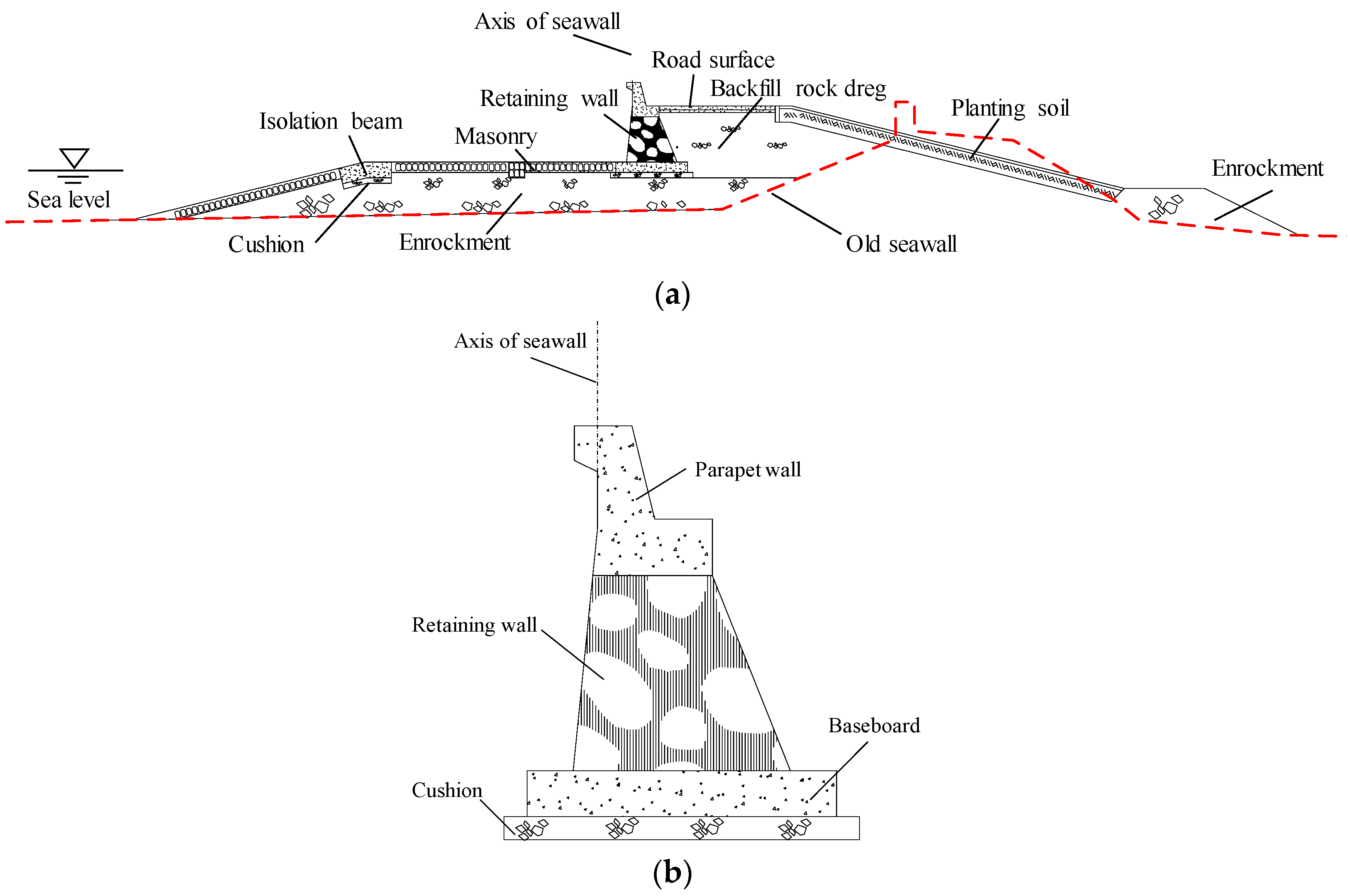
4.1. Project Overview

A certain seawall is located in the coastal region of Southeast China. The project consists of two embankments and two sluices, with a total length of 1.46 km. The seawall is categorized as Class III engineering, and the level of the main structures is three. The construction of the project was completed in 2015. The schematic of the seawall is shown in Figure 7. The automatic monitoring system was installed in the seawall, with a monitoring section per 500 m along the alignment. Each section set up three surface deformation monitoring points. A total of 108 deformation monitoring points were set on the surface of the seawall.

In this case study, we selected the settlement monitoring data of monitoring points N1, N3, N9, N12, and N14 installed in various seawall sections from 10 January 2023 to 15 February 2023 for analysis. It determined that the vertical downward is positive, and the vertical upward is negative for seawall settlement monitoring data. The original monitoring data was pre-processed to detect outliers at first. One settlement monitoring data can be obtained per five minutes. The settlement monitoring data of the selected monitoring points are exhibited in Figure 8. It can be drawn from Figure 8 that the settlement monitoring data appeared to have obvious daily periodic variation regularity. The maximum settlement generally occurred at 12 o’clock at noon each day, and the minimum settlement appeared at 0 o’clock the next day. As is illustrated in Figure 8, the seawall settlement and upstream water level data series of monitoring points all represent a certain correlation.

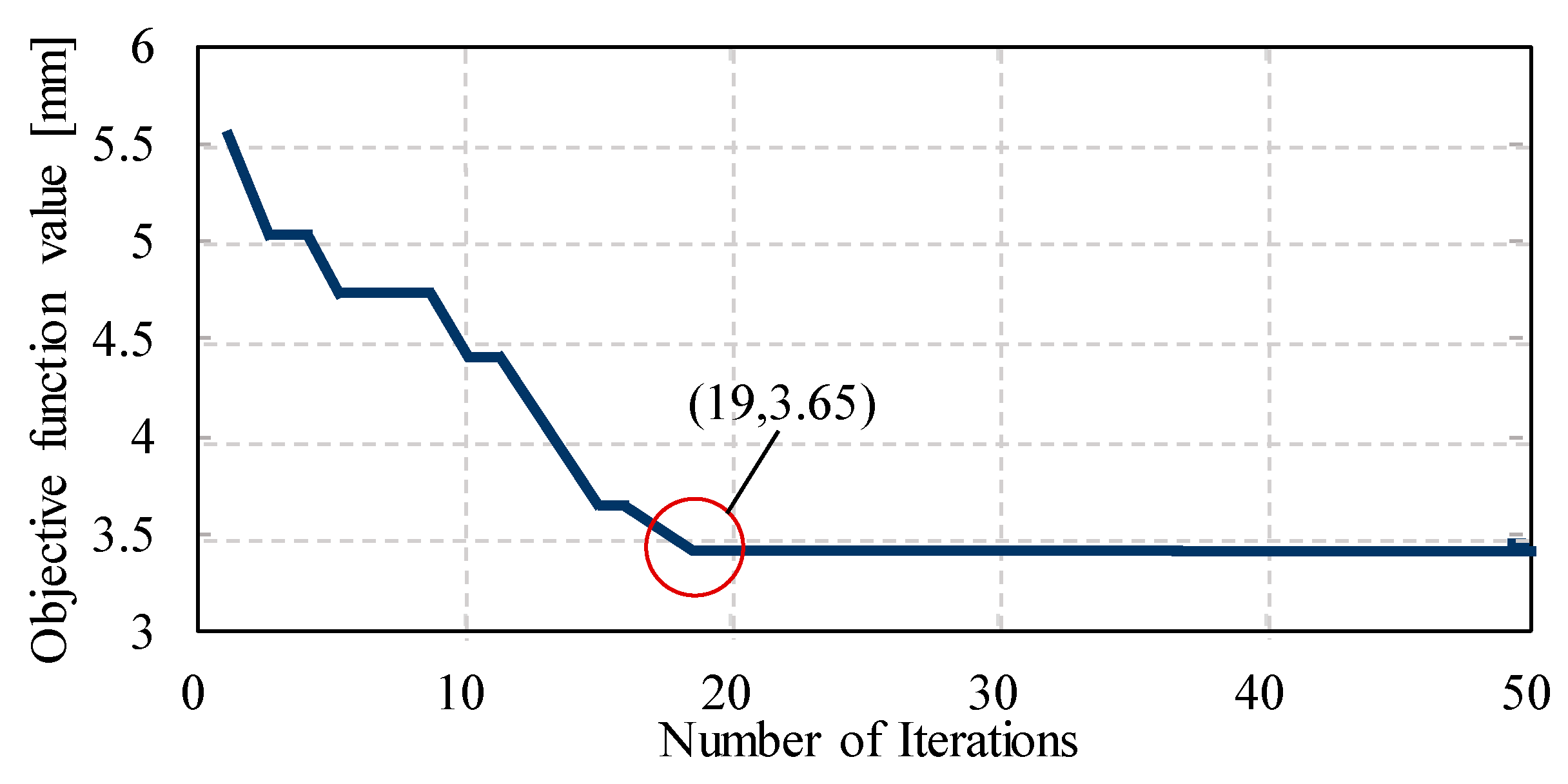
4.2. Major Influencing Factor Determination Based on CPSO-MNN

Based on the analysis of influencing factors and seawall settlement components in Section 3.1.1, the data of all the settlement components were normalized. Therefore, water pressure, water level variation lagging effect, temperature, time effect, wind speed, and tide were considered as influencing factors of seawall settlement. Parameter initialization of the WNN model was carried out primarily; the number of input factors N was set to 6, the number of hidden layer nodes M was set to 4, and the number of output nodes was 1. In order to determine the optimal structure of WNN, the WNN model was utilized to predict seawall settlement of various monitoring points. The average mean square error (MSE) between the predicted value and measured value of the seawall settlement of five monitoring points was used to evaluate the prediction precision of the WNN model. Additionally, it can be noticed in Figure 9 that when adopting the “6-4-1” structure, the WNN model presented the best prediction ability. Therefore, the “6-4-1” structure is employed in the WNN model construction. In addition, CPSO is adopted to optimize the input weight, output weight, extension factor and translation factor of WNN. The number of extension factors and translation factors of the wavelet function were both set to 4. The number of particles was set between 20 to 50. Once the initial particle set was established, the WNN model was trained by using 20, 30, and 40 particles, respectively. It was suggested that when the number of particles was set to 40, the learning factor and were both set to 2, and the maximum iteration times were set to 300, the most satisfactory training result was obtainable. The fitness value curves of CPSO and the gradient decent method applied in traditional parameter selection of the WNN model were compared in Figure 10. It can be found that CPSO possesses the advantages of shortening the iterative time and increasing rapidly in convergence.

Eventually, the normalized importance value R of various influencing factors for different monitoring points is shown in Figure 11. In Figure 11, temperature and time both had a weak influence on seawall settlement; therefore, they cannot be regarded as major influencing factors. The reason behind this phenomenon was mainly attributed to the fact that the seawall is located in a mild region, where temperature variation has a relatively slight effect on the seawall settlement. Further, the time span of seawall settlement monitoring data covers only one month, and the measured values cannot exhibit an obvious trend over time. As a result, the time effect did not exert a noticeable influence on the monitoring effect.

4.3. Analyses of Fitting and Prediction Results

In this study, the initial particles of CPSO were set to 40, c₁ and c₂ were both 2. The number of iterations was set to 50. Additionally, the Mean Absolute Error (MAE) was adopted as the fitness function, which can be determined by:

$$MAE=\frac{{\displaystyle \sum _{i=1}^N\left|{\widehat{\delta }}_i-{\delta }_i\right|}}{N}$$

(49)

The parameters in Equation (49) have the same meaning as in Equation (47)

Figure 12 depicts the objective function value of CPSO at each iteration. It can be seen that the objective function reached the minimum value at 19 iterations. Finally, the optimal learning rate was 0.025, and the optimal number of hidden layers and hidden nodes were 3 and 6, respectively.

4.3.1. The Variables Inputted in the Prediction Model

Hereby, the expression of the seawall settlement model according to the major influencing factor determination result can be expressed as:

$$\delta =a_0+{\displaystyle \sum _{i=0}^3{a}_{1i}{H}^i}+{\displaystyle \sum _{i=1}^{m_1}{a}_{2i}}{\overline{H}}_i+{\displaystyle \sum _i^{m_3}{f}_i}{V}^i+k_1\cos (\frac{2\pi t}{24})+k_2\sin (\frac{2\pi t}{24})$$

(50)

The parameters in Equation (50) have the same meaning as in Equation (38).

4.3.2. Analyses and Comparisons of the Fitting and Prediction Performance

In order to establish the seawall settlement prediction model by applying LSTM, the settlement monitoring data series were grouped into a training sample (75% of the data) and a test sample (25% of the data). Therefore, the seawall settlement data from 10 January 2023, 5:51, to 8 February 2023, 5:19, were employed to establish the prediction models of various settlement monitoring points. Meanwhile, the seawall settlement data from 8 February 2023, 5:24, to 15 February 2023, 23:42, were applied to test the models.

In addition, there are three different types of prediction models based on training samples by using the LSTM and the BPNN according to Equation (38). The fitting and prediction results of the LSTM model, the Back Propagation Neural Network (BPNN) model, and the proposed model of five monitoring points are exhibited in Figure 13. In the locally enlarged images, three models fitted most of the monitoring data well; the over-fitting problems did not exist in the three models. The R² and RMSE of three models for different monitoring points were calculated, and the statistical results are illustrated in

Table 1. The R² and RMSE of the LSTM, BPNN model, and the proposed model.

Monitoring Point	LSTM		BPNN		The Proposed Model
	R2	RMSE [mm]	R2	RMSE [mm]	R2	RMSE [mm]
N1	0.9765	0.0172	0.9655	0.0182	0.9976	0.0032
N3	0.9740	0.0173	0.9698	0.0251	0.9956	0.0147
N9	0.9880	0.0062	0.9750	0.0167	0.9902	0.0061
N12	0.9761	0.0065	0.9777	0.0161	0.9921	0.0064
N14	0.9769	0.0061	0.9409	0.0197	0.9801	0.0049

.

As shown in Table 1, the R² of LSTM, BPNN, and CPSO-WNN-LSTM models varies from 0.9740 to 0.9880, from 0.9409 to 0.9777, and from 0.9801 to 0.9976, respectively. For five monitoring points, the values of RMSE of the CPSO-WNN-LSTM model are the smallest, which verifies the most excellent prediction accuracy of the CPSO-WNN-LSTM model. In order to analyze intuitively the superiority of the proposed model, the fitting and prediction residuals of three prediction models for five typical settlement monitoring points are depicted in Figure 14. The partially enlarged views demonstrate the prediction results of the models based on test samples.

Figure 14 describes the fitting and prediction residuals of three models by the residual area plots, which clearly exhibit the positive and negative fluctuations of all residuals. Nevertheless, it can be seen that in contrast to the other two prediction models, the fluctuation of the CPSO-WNN-LSTM model is the smallest. Owing to the extraordinary learning and memory abilities of the LSTM model, the variation of the residuals of the LSTM model and the proposed model both represented relatively stable over time. However, because the proposed model took the major influencing factors into full consideration and optimized the parameters of LSTM sufficiently, the value of the residuals of the CPSO-WNN-LSTM was the smallest of all the models in most of the monitoring time.

5. Conclusions

Recently, the seawall deformation problem has aroused public awareness in China. However, the valid seawall deformation prediction model still has been rarely studied. In this study, in-depth research efforts have been devoted to seawall deformation prediction methods to contribute to seawall structural health evaluation. Primarily, the chaos optimization is incorporated into PSO to generate the CPSO algorithm. Afterward, the parameters of the WNN model are optimized by implementing CPSO to determine major influencing factors of seawall deformation. On this basis, the training samples are inputted into the LSTM model to establish a prediction model of seawall deformation. With the aim of enhancing the model construction efficiency, the CPSO is introduced to optimize the parameters of LSTM in advance. Eventually, the prediction performance of the proposed prediction model is verified using a specific case study. The main content of the study leads to the following conclusions:

(1) A crucial question with regard to improving the prediction accuracy of seawall deformation is to determine the major influencing factors of seawall deformation. Therefore, the potential influencing factors have been further studied in this research. Additionally, the seawall deformation components caused by water pressure, water level variation lagging effect, temperature, time effect, wind speed, and tides are characterized clearly. Given the strong nonlinear mapping capability of WNN, the WNN model is implemented to resolve the problem of major influencing factor determination. In order to optimize the structure of the WNN model, CPSO is adopted to optimize the WNN model. The actual application results demonstrate that the CPSO performs a better optimization ability than the gradient decent method applied in traditional parameter selection of the WNN model.

(2) According to the major influencing factor determination results, the LSTM model optimized by CPSO is introduced to establish the seawall prediction model. The values of R² of the CPSO-WNN-LSTM model for different point covers range from 0.9801 to 0.9976. In contrast to the LSTM and BPNN models, the proposed method has the smallest values of RMSE of prediction results. The analyses of the case study demonstrate that the CPSO-WNN-LSTM model exhibits superior prediction performance, which illustrates the importance of major influencing determination and the excellent prediction ability of long-term data series.

The study provides a new insight into the seawall deformation prediction. Further, extensive validation should be carried out in more engineering projects to verify the applicability and generality of the proposed model.

References

1. Shao, C.; Gu, C.; Meng, Z.; Hu, Y. A data-driven approach based on multivariate copulas for quantitative risk assessment of concrete dam. J. Mar. Sci. Eng. 2019, 7, 353. [Google Scholar] [CrossRef]
2. Lan, Z.; Huang, M. Safety assessment for seawall based on constrained maximum entropy projection pursuit model. Nat. Hazards 2018, 91, 1165–1178. [Google Scholar] [CrossRef]
3. Lan, Z.; Huang, M. Health assessment model and maintenance decision model for seawall prognostics and health management system. Arab. J. Sci. Eng. 2019, 44, 8377–8387. [Google Scholar] [CrossRef]
4. Ning, D.; Wang, R.; Chen, L.; Li, J.; Zang, J.; Cheng, L.; Liu, S. Extreme wave run-up and pressure on a vertical seawall. Appl. Ocean Res. 2017, 67, 188–200. [Google Scholar] [CrossRef]
5. Huang, M.; Liu, J. Monitoring and analysis of Shanghai Pudong seawall performance. J. Perform. Constr. Facil. 2009, 23, 399–405. [Google Scholar] [CrossRef]
6. Yu, Q.; Wang, Q.; Yan, X.; Yang, T.; Song, S.; Yao, M.; Zhou, K.; Huang, X. Ground deformation of the Chongming East Shoal Reclamation Area in Shanghai based on SBAS-InSAR and laboratory tests. Remote Sens. 2020, 12, 1016. [Google Scholar] [CrossRef]
7. Dixon, T.H.; Amelung, F.; Ferretti, A.; Novali, F.; Dokka, R.; Sella, G.; Kim, S.W.; Wdowinski, S.; Whitman, D. Subsidence and flooding in New Orleans. Nature 2006, 441, 587–588. [Google Scholar] [CrossRef]
8. Pei, Y.; Liao, M.; Wang, H. Monitoring levee deformation with repeat-track space-borne SAR images. Geomat. Inf. Sci. Wuhan Univ. 2013, 38, 266–269. [Google Scholar]
9. Zhang, Y.J.; Wan, Z.; Xie, C.; Shao, Y.; Yuan, M.H.; Chen, W.; Wang, X. Deformation analysis of the seawall in Qiantang estuary with multi-temporal InSAR. J. Remote Sens. 2015, 19, 339–346. [Google Scholar]
10. Qin, X.; Xie, L.; Wang, C.; Liao, M. 3D deformation monitoring and analysis of coastal seawall combined with multi-view InSAR measurements. In Proceedings of the IGARSS 2022—2022 IEEE International Geoscience and Remote Sensing Symposium, IEEE, Kuala Lumpur, Malaysia, 17–22 July 2022; pp. 1648–1651. [Google Scholar]
11. Wang, G.; Li, P.; Li, Z.; Ding, D.; Qiao, L.; Xu, J.; Li, G.; Wang, H. Coastal dam inundation assessment for the Yellow River Delta: Measurements, analysis and scenario. Remote Sens. 2020, 12, 3658. [Google Scholar] [CrossRef]
12. Oh, Y.N.; Chien, L.K.; Chen, S. Deformation and settlement analysis of foundation in seawalls using DDA. In Proceedings of the Ninth International Offshore and Polar Engineering Conference, ISOPE, Brest, France, 30 May–4 June 1999. [Google Scholar]
13. Kanatani, M.; Kawai, T.; Tochigi, H. Prediction method on deformation behavior of caisson-type seawalls covered with armored embankment on man-made islands during earthquakes. Soils Found. 2001, 41, 79–96. [Google Scholar] [CrossRef] [PubMed]
14. Jiang, H.; Wang, L.; Li, L.; Guo, Z. Safety evaluation of an ancient masonry seawall structure with modified DDA method. Comput. Geotech. 2014, 55, 277–289. [Google Scholar] [CrossRef]
15. Qin, P.; Qin, Z.H. Prediction of seawall foundation settlement based on the improved variable dimension fraction and artificial neural network model. In Proceedings of the 2010 2nd International Conference on Advanced Computer Control, IEEE, Shenyang, China, 27–29 March 2010; pp. 347–350. [Google Scholar]
16. Qin, P.; Cheng, C. Prediction of seawall settlement based on a combined LS-ARIMA model. Math. Probl. Eng. 2017, 2017, 7840569. [Google Scholar] [CrossRef]
17. Ma, J.Q.; Wang, X.G.; Pei, C.Y. Research on the seawall settlement based on BP neural network. Chin. Water Transp. 2017, 17, 225–227. (In Chinese) [Google Scholar]
18. Yu, H.; Wu, Z.R.; Bao, T.F.; Zhang, L. Multivariate analysis in dam monitoring data with PCA. Sci. Chin. Technol. Sci. 2010, 53, 1088–1097. [Google Scholar] [CrossRef]
19. Lei, W.; Wang, J. Dynamic Stacking ensemble monitoring model of dam displacement based on the feature selection with PCA-RF. J. Civ. Struct. Health Monit. 2022, 12, 557–578. [Google Scholar] [CrossRef]
20. Dai, B.; Gu, C.; Zhao, E.; Qin, X. Statistical model optimized random forest regression model for concrete dam deformation monitoring. Struct. Control Health Monit. 2018, 25, e2170. [Google Scholar] [CrossRef]
21. Yang, Z.; Ye, Q.; Chen, Q.; Ma, X.; Fu, L.; Yang, G.; Yan, H.; Liu, F. Robust discriminant feature selection via joint L2, 1-norm distance minimization and maximization. Knowl.-Based Syst. 2020, 207, 106090. [Google Scholar] [CrossRef]
22. Gu, H.; Yang, M.; Gu, C.; Huang, X. A factor mining model with optimized random forest for concrete dam deformation monitoring. Water Sci. Eng. 2021, 14, 330–336. [Google Scholar] [CrossRef]
23. Hochreiter, S.; Schmidhuber, J. Long short-term memory. Neural Comput. 1997, 9, 1735–1780. [Google Scholar] [CrossRef]
24. Hu, Y.; Gu, C.; Meng, Z.; Shao, C.; Min, Z. Prediction for the settlement of concrete face rockfill dams using optimized LSTM model via correlated monitoring data. Water 2022, 14, 2157. [Google Scholar] [CrossRef]
25. Bolboacă, R.; Haller, P. Performance analysis of long short-term memory predictive neural networks on time series data. Mathematics 2023, 11, 1432. [Google Scholar] [CrossRef]
26. Zhang, Q.; Benveniste, A. Wavelet networks. IEEE Trans. Neural Netw. 1992, 3, 889–898. [Google Scholar] [CrossRef] [PubMed]
27. Kennedy, J.; Eberhart, R.C. Particle swarm optimization. In Proceedings of the IEEE International Conference on Neural Networks, Perth, Australia, 27 November–1 December 1995; pp. 1942–1948. [Google Scholar]
28. Chen, Z.; Xiong, R.; Wang, K.; Jiao, B. Optimal energy management strategy of a plug-in hybrid electric vehicle based on a particle swarm optimization algorithm. Energies 2015, 8, 3661–3678. [Google Scholar] [CrossRef]
29. Zhang, L.; Zhang, W.; Liu, J.; Zhao, T.; Zou, L.; Wang, X. A new prediction model for transformer winding hotspot temperature fluctuation based on fuzzy information granulation and an optimized wavelet neural network. Energies 2017, 10, 1998. [Google Scholar] [CrossRef]
30. Zhang, D. A new approach for the efficient estimation of the number of hidden unites for feedforward neural networks. Comput. Eng. Appl. 2003, 5, 21–23, 95. (In Chinese) [Google Scholar]
Figure 1. The schematic diagram of one cross-section of a current seawall and the old seawall in China. (a) A typical section. (b) The detail of the retaining wall of our sea.
Mathematics 11 03752 g001
Figure 2. The structure of the WNN.
Mathematics 11 03752 g002
Figure 3. Three possible moving directions.
Mathematics 11 03752 g003
Figure 4. The process of the major influencing factor determination is based on the CPSO-WNN model.
Mathematics 11 03752 g004
Figure 5. Structure of LSTM.
Mathematics 11 03752 g005
Figure 6. The flowchart of the seawall deformation prediction model construction process.
Mathematics 11 03752 g006
Figure 7. (a) The layout diagram of the seawall layout, (b) photo of the seawall upstream side.
Mathematics 11 03752 g007
Figure 8. Water level and settlement monitoring data series of: (a) N1, (b) N3, (c) N9, (d) N12, and (e) N14.
Mathematics 11 03752 g008
Figure 9. The prediction MSE of various structures of the WNN model.
Mathematics 11 03752 g009
Figure 10. Fitness value curves of CPSO and the gradient decent method.
Mathematics 11 03752 g010
Figure 11. Normalized importance value R of various influencing factors for each monitoring point.
Mathematics 11 03752 g011
Figure 12. The objective function values at each iteration.
Mathematics 11 03752 g012
Figure 13. The fitting and prediction results of three models for different monitoring points: (a) N1, (b) N3, (c) N9, (d) N12, (e) N14.
Mathematics 11 03752 g013aMathematics 11 03752 g013b
Figure 14. The fitting and prediction residuals of three models for different monitoring points: (a) N1, (b) N3, (c) N9, (d) N12, and (e) N14.
Mathematics 11 03752 g014