Abstract
The Transfer-Matrix Method (TMM) is an original and relatively simple mathematical approach for the calculus of thin-walled cylindrical tubes presented in this work. Calculation with TMM is much less used than calculation with the Finite Elements Method (FEM), even though it is much easier to apply in different fields. That is why it was considered imperative to present this original study. The calculus is based on Dirac’s and Heaviside’s functions and operators and on matrix calculation. The state vectors, the transfer-matrix, and the vector corresponding to the external efforts were defined, which were then used in the calculations. A matrix relation can be written, which gives the state vector of the last section depending on the state vector of the first section, a relation in which the conditions of the two end supports can be set. As an application, a heat exchanger was studied, with a large cylinder subjected to a uniformly distributed internal load, and from the inner cylinder bundle, a cylinder subjected to both uniform internal and external loads was considered. For the second cylinder, two possibilities of action for the external forces were considered, a successive action and a simultaneous action, achieving the same results in both situations. The TMM is intended to be used for iterative calculus in optimization problems where rapid successive results are required. In the future, we want to expand this method to other applications, and we want to develop related programs. This is an original theoretical study and is a complement to the research in the field on thin-walled cylinder tubes and their applications in heat exchangers.
Keywords:
mathematical model of thin-walled cylindrical tube; load density; state vector; Transfer-Matrix Method; Dirac’s function; Heaviside’s function MSC:
74-10
1. Introduction
The Transfer-Matrix Method (TMM) is based on a mathematical formalism that facilitates the solution of many engineering problems through the possibility of very easily programming the calculation algorithm. The TMM is very easy to apply for iterative problems, especially for the optimization calculation of the shape of different pieces.
This article presents an original approach to the calculation of a model of cylinder tubes subjected to different uniformly distributed forces using the TMM.
The objective of this study was to determine the calculation formulas using the Transfer-Matrix Method (TMM) for the case of a long thin-walled cylinder tube loaded with a uniformly distributed internal load embedded at both ends and for the case of a long thin-walled cylinder tube loaded with a uniformly distributed external load, embedded at both ends, with direct application to a heat exchanger. This approach can be programmed relatively easily, being iterative calculations, and can facilitate the numerical solution of shape optimization problems that require immediate results (we hope to be able to present such numerical results in future articles).
The basic elements for the calculus of different structures using TMM are presented in [1], and the resistance calculations for the different structures are presented in [2]. In [3], the application of TMM to the reproduction of an antireflection layer is given. The transfer-matrix factorization for symmetric optical systems is shown in [4]. In [5], multilayered cylinders made of functionally graded materials are studied using the TMM. The solution of an FGM thick-walled cylinder with an arbitrary inhomogeneous response via TMM is presented in [6]. In [7], the coupling of TMM with FEM (Finite Elements Method) is given for the acoustic analysis of complex networks of hollow bodies. Ref. [8] gives a formula for the intrinsic transfer-matrix, and [9] gives some theoretical and experimental extensions based on the properties of the intrinsic transfer-matrix. Applications for the measurement of a single-crystal elasticity matrix of polycrystalline materials are presented in [10]. Ref. [11] gives a modified differential TMM for the solution of one-dimensional linear inhomogeneous optical structures. In [12], an improved differential TMM for inhomogeneous one-dimensional photonic crystals is given, and a general solution of linear differential equations using a differential TMM is shown in [13]. Some Transfer-Matrix Methods for sound attenuation in resonators with perforated intruding inlets are given in [14]. A Stiffness Transfer-Matrix Method (STMM) for the solution of stable dispersion curves in anisotropic composites is presented in [15]. An analytical solution of linear ordinary differential equations via a differential TMM is shown in [16,17], and a differential TMM for the solution of one-dimensional linear non-homogeneous optical structures is given. A matrix method for elastic wave problems is presented in [18]. The characterization and development of periodic acoustic meta-materials using a transfer-matrix approach are given in [19,20], and a modified TMM for the prediction of transmission loss in multilayered acoustic materials is shown. Another application of TMM is presented in [21] to estimate the noise transfer-matrix related to the combustion of a multi-cylinder diesel engine. In [22], a minimal optical decomposition of ray transfer-matrices is shown. Matrix techniques for modeling ultrasonic waves in multilayered media are given in [23]. The formulation of a differential TMM for cylindrical geometry is presented in [24]. A simplified modal analysis based on the properties of the transfer-matrix is given in [25]. In [26], a diffuse field transmission via multilayered cylinders using a TMM is shown. The rendering of transfer-matrix-based layered materials is presented in [27]. A geometrical perspective on the TMM is given in [28]. An analysis of wave propagation in functionally graded porous cylindrical structures considering the TMM is presented in [29]. Ref. [30] gives a derivation of the phase differences of nonsymmetrical interferometers using partitioned transfer-matrices. In [31], the TMM can be seen being used for four-flux radiation, and in [32], a transfer-matrix approach is given for estimating the characteristic impedance and wave numbers of limp and rigid porous materials. In [33], an approach is presented for some elements of the calculus of long thin-walled cylindrical tubes via TMM. In [34], a very interesting approach using the TMM for the calculus of mandible bone is shown. The TMM applied to the parallel assembly of sound-absorbing materials is shown in [35]. An integrated TMM for multiple connected mufflers is given in [36]. A differential transfer- matrix based on Airy’s functions in the analysis of planar optical structures with arbitrary index profiles is presented in [37]. A collection of formulas for stresses and strains is given in [38]. Ref. [39] presents a fractional thermal transport and twisted light induced by an optical two-wave mixing in single-wall carbon nanotubes. The Transfer-Matrix Method in the context of acoustical wave propagation in wind instruments is presented in [40].
The novelty and the originality of this work consist of using a long cylindrical tube with thin walls loaded with the load uniformly distributed inside and/or outside and embedded at both ends. The novelty and originality also include the studied industrial application, i.e., a heat exchanger. FEM needs a large computing power to obtain correct results. The mathematical formulation with the help of TMM is easy to program, being much simpler to apply to obtain the same accuracy of the results, with a much higher calculation speed and thus with a significant gain in the allocated time. This is an advantage compared to FEM, which explains our interest in TMM. The TMM, based on Dirac’s and Heaviside’s functions and operator with the formulas derived in this study, can be used for calculating the stresses and deformations in any section of a piece. In this case, a single thin wall cylinder tube is required by a load uniformly distributed inside and/or outside. The applicability perspective of our study to cylindrical nanotubes is very interesting, too [39], and in the future, we will try to study these cases of cylinders as well.
2. Materials and Methods
2.1. Materials
For the industrial applications that we thought of studying in this work, the materials recommended for making cylinders must have special mechanical characteristics and, at the same time, present very good thermal properties. Since we are talking about large temperature variations and very different fluids, which will demand the cylinders both inside and outside, the materials used in the manufacture of the cylinders must be of very good quality and comply with the required reliability and availability conditions. Depending on the needs, the following materials can be used: stainless steel, alloyed or not with titanium, copper, wolfram, molybdenum, special steels alloyed with titanium, nickel, copper, aluminum alloys with silicon, and small amounts of copper, iron, nickel, zinc, magnesium, manganese, duralumin, ceramic materials, graphite, composite materials based on graphite or fluoroplastic, etc.
2.2. Methods
The mathematical apparatus used in this original research is based on the principles developed in [1], where the basics of TMM are presented, and the calculus of the Resistance of Materials is presented in [2]. A calculus attempt for cylinder tubes is presented in [33]. This calculus needs some working hypotheses.
2.2.1. Working Assumptions
The study of a cylindrical and thinly tube is made with the following working assumptions [1]:
- Under the action of external forces perpendicular to the average plane, the curvature varies;
- The curvature variation occurs in two planes, forming an elastic surface with double curvature;
- The shape of the elastic surface is characterized by the variation law of the arrow
- f(x, y), in Cartesian coordinates;
- It is assumed that the numerical values of the function f(x, y) are very small in relation to the thickness h;
- The points aligned on the same normal to the average surface before the deformation remain aligned on the same normal to the deformed surface and after deformation;
- The normal stresses in the sections parallel to the median plane are negligible in relation to the bending stresses;
- Normally continue to remain invariable after deformation;
- For a long cylindrical tube, the stresses and the deformations have a revolution’s symmetry;
- The cylinder is defined in a fixed coordinate axis system; the Ox axis is directed according to the generators, the Oy axis is directed according to a radius, and the Oz axis is taken in such a way that the triaxial system Oxyz is directly.
2.2.2. Fundamental Equations for a Long Cylinder
The fundamental equations for a model of long cylinder will be deducted for the cylinder presented in Figure 1. It is considered a model of cylindrical tube with a thin wall, the thickness is h, the radius is R, and length is l, [1], with an axisymmetric uniform load at all interior surfaces of the tube, defined using load density q(x), (Figure 1).
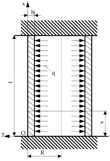
Figure 1.
Model of cylindrical tube with axisymmetric interior uniform load.
The load density, with Dirac’s and Heaviside’s functions (for Figure 1), can be written as the following relation (1):
where Y(x) is the Heaviside function.
The abscissas are measured from the origin O, positive in the sense of the external normal to the cylinder. The stresses and deformations that arise in the cylinder also show a symmetrical evolution.
It is written with f as the arrow or the radial displacement and φ as the angle between the tangent and the initial generator of the cylinder.
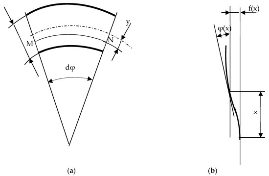
Figure 2.
Deformations: (a) Deformed MN fiber. (b) Deformations: arrow—f(x) and rotation—φ(x).
It can be written as follows (2) for the deformation f(x):
Figure 2a represents the deformed thickness h of the cylinder and a cubic segment MN located at a distance y from the median surface. The three-axial orthogonal system is fixed as follows: Ox is after the cylindrical tube’s generator, Oy is after a radius, and axis Oz is oriented as the system Oxyz will be a direct system. The relative deformation of MN is expressed as follows (3):
where is the deformation of the middle fiber. The circumferential deformation is expressed as follows (4):
The following stresses (5) correspond to these deformations, as shown in [2]:
where E is Young’s modulus, and ν is Poisson’s coefficient.
If Equations (3) and (4) are replaced in (5), Equation (6) for stresses are obtained as follows:
For an element of the cylindrical tube, it is noted that dx—the length and ds—the breadth (Figure 3).
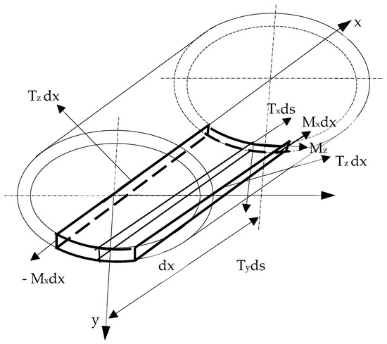
Figure 3.
An element dx of a long cylinder wall tube.
For the cutting forces Tx and Tz, it can be written as follows (7):
or (8):
For the flexion moments Mx and Mz, it can be written as (9):
or (10):
when, (11) give:
With (11), (8) becomes (12):
For the element dx, the balance equations are written as follows in which the projection equation on Ox is (13):
which yields (14):
The projection equation on Oy is (15):
which yields (16):
The moment equation is (17):
with (18):
It can still be written as (19):
and (20):
Tz between Equations (19) and (20) is eliminated, and we obtain (21):
It also takes into account that (22):
the equation for the cylinder is (23):
with the notation (24):
So, the following relations (25) allow us to calculate the deformation and stresses in a thin cylindrical wall tube:
The general solution of Equation (23) is (26):
where f∗(x) is the particular solution for the equation with second member, and Ai, i = 1, 4 are the constants from solution (26).
2.2.3. The Transfer-Matrix for a Long Cylindrical Thin Wall Tube
It is considered a long cylindrical thin wall tube embedded at the inferior end and at the superior end (Figure 1). State vectors and transfer-matrix can be defined as follows.
The state vector {U(x)} is defined at the x-axis point in Equation (27):
The state vector in the origin section, at the section 0, in the inferior end, is (28):
and the state vector in the last section, section l, in the superior end, is (29):
The state vector (27) is linked to the state vector (28) via a matrix relation (30):
with a transfer-matrix [T]x, having the form given as follows (31):
and the vector {Ux}e corresponding to the external forces on element x is (32):
with the notations in (33) for ki(x − t), i = 1, 4, which are the values of the function ki in the point (x − t) expressed as follows:
and with their derivatives (34):
At the superior end, for x = l, it can be written as follows (35):
The matrix relation (35) can be written in the form given as (36) for section l:
where the vector {Ul}e takes different forms depending on the external loads.
3. Application and Results
We thought that our calculus with the formalism given via TMM can be used for a heat exchanger, which has a large cylinder requiring a uniformly distributed internal force and a bundle of cylinders located inside the large cylinder that requires both a uniformly distributed external force and a uniformly distributed internal force (Figure 4a–c).
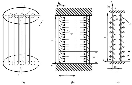
Figure 4.
Model of heat exchanger. (a) Model of heat exchanger; (b) exterior cylinder 1 charged; (c) interior cylinder 2 charged.
Thus, the two following cases will be studied: a cylinder subjected to a uniformly distributed internal force (cylinder 1), embedded at both ends, (Figure 4a,b), and a cylinder subjected to both a uniformly distributed internal force and a uniformly distributed external force, embedded at both ends (cylinder 2), (Figure 4a,c).
3.1. Long Thin Cylindrical Wall Tube Charged with an Interior Axisymmetric Uniform Distributed Load and Embedded at Both Ends (Figure 4b)
For Figure 4b, and with index 1 for this cylinder, the load density can be written as follows (37), with Dirac’s and Heaviside’s functions:
Equation (25), for the application from Section 3.1, can be written as follows (38):
with notation (39):
and (40):
Equation (41) is expressed as follows:
Solution is written as follows (42):
where A1i, i = 1, 4 are the constants from general solution (42).
For the application from Section 3.1, the state vector is defined at the x-axis section as follows (43):
The state vector in the origin section, at the section 0, for the inferior end, is as follows (44):
and the state vector in the last section, section l, in the superior end, is as follows (45):
The state vector (44) is linked to the state vector (45) via a matrix relation as follows (46):
Transfer-matrix [T1]x is given as follows (47):
and the vector {U1x}e corresponding to the external forces on element x, is as follows (48):
with the following notations in (49) for k1i (x − t), i = 1, 4, which are the values of the function k1i in the point (x − t):
and with their derivatives (50):
At the superior end, for x = l, it can be written as follows (51):
The matrix relation (51) can be written as given in (52) for section l:
or (53):
We have the edge’s conditions as follows(54):
With (54), Equation (53) will be elucidated as follows (55):
The calculus of the two elements of the origin state vector, M1x0 and T1y0, can be written, after matrix relation (55), as the linear system of Equation (56):
or (57):
with solution (58):
and notations (59):
Now, the two unknown elements of the state vector of the last face can be calculated from the matrix relation (55). The solutions can be written as follows (60):
At this moment, the elements of the two state vectors of sections at the two ends of the cylinder, loaded with the uniformly distributed internal load, are recognized. With matrix relation (46), it can be calculated, and thus, we have all the elements of the origin’s state vector. Then, we can calculate all the state vectors for all the sections of the long cylindrical tube.
3.2. Long Thin Cylindrical Wall Tube Charged with an Exterior and Interior Axisymmetric Uniform Distributed Load (Figure 4c)
The long cylindrical thin wall tube is considered to be charged with an axisymmetric interior uniform load for the interior surface of cover q2 and an exterior uniform load for the exterior surface q3, which is embedded at the origin (inferior end) and at the superior end (Figure 4c).
The load density, with Dirac’s and Heaviside’s functions, for Figure 4 is as follows (61):
The calculus of this cylinder can be calculated in two ways, which will be presented as follows:
- The calculus of this cylinder under the successive action of the external efforts with the superimposing effects for the successive action of the external efforts on a cylinder;
- The calculus of this cylinder under the simultaneous action of the external efforts.
For this cylinder with double loading, the following indexes will be used: for the mechanical and geometric characteristics, index 2 will be used for internal loading, and for external loading, index 3 will be used.
3.2.1. Calculus of Cylinder under Successive Action of External Efforts
Interior Load q2
The load density, with Dirac’s and Heaviside’s functions, (for Figure 4c), can be written as follows (62):
It is noted as follows (63):
and (64):
Equation (65) is expressed as follows:
Ssolution is (66):
where A2i, i = 1, 4 are constants from the general solution presented in Equation (66).
For the application from Section “Interior Load q2”, the state vector is defined at the x-axis section as follows (67):
The state vector (67) is linked to the state vector in the origin (inferior end) as the following matrix relation (68):
Transfer-matrix [T2]x is given as follows (69):
and the vector {U2x}e corresponding to the external forces on element x is expressed as follows (70):
with the notations in (71) for k2i(x − t), i = 1, 4 in the point (x − t) written as follows:
and with their derivatives (72):
At the superior end, for x = l, it can be written as follows (73):
The matrix relation (73) can be written as Equation (74) for section l:
or (75):
We have for the two embedded edges, with the edge’s conditions written as follows (76):
With (76), the relation (75) will be (77):
The calculus of the two elements of the origin state vector, M2z0 and T2y0, can be written, after matrix relation (56), as the linear system of Equation (78):
or (79):
with solution (80):
and notations (81):
Now, we can calculate the two unknown elements of the state vector corresponding to the last face (superior end) from the matrix relation (77). We can write the solutions as follows (82):
Exterior Load q3
For the exterior load q3, the same steps are followed as for the internal load, but it must be taken into account that it is of the opposite sign compared to the internal load. It is the same as the cylinder presented in Section “Interior Load q2”, but with the index 3, corresponding to this load.
The load density, with Dirac’s and Heaviside’s functions, is expressed as follows (83):
For this cylinder, we can write the matrix relation as follows (84):
Following equation uses the same notations in (64), (65), (72) and (73). Because we have the same cylinder, the transfer-matrix [T3]x is given as Equation (85), the same as Equation (70):
The vector {U3x}e corresponding to the external forces on element x is as follows (86):
At the superior end, for x = l, it can be written as follows (87):
The edge’s conditions are expressed as follows (88):
With (88), the relation (87) will be (89):
The calculus of the two elements of the origin state vector, M3z0 and T3y0, can be written as the linear system of Equation (90):
or (91):
with solution (92):
and notations (93):
We can write for the two elements M3x(l) and T3y(l), the solutions (94):
The Method of the Superimposing Effects for Successive Action of External Efforts on a Cylinder
This method is currently used in the Strength of Materials calculus [2]. Superimposing the effects of the successive action of external efforts for the cylinder from Figure 4c, we can write (95):
or (96):
and for the last end, we can write (97):
or (98):
3.2.2. Calculus of Cylinder under Simultaneous Action of External Efforts
This time, the forces act simultaneously, according to It is not recommended to write the previous formula again to avoid repeating the formula and numbering the wrong order (not in numerical order). The load density, with Dirac’s and Heaviside’s functions, for Figure 4c, can be written as Equation (61), which is simultaneous for the two external loads.
Equations (27)–(29) remain the same. Because it is the cylinder 2 loaded simultaneously with both forces, the matrix relation (30) becomes (99):
Transfer-matrix [T′]x is given as follows (100):
and the vector {Ux′}e corresponding to the two external forces on element x is as follows (101):
Because it is the cylinder 2 loaded simultaneously with both forces, the notations in (63), (64), (71) and (72) are kept. The matrix relation (99) can be written as follows (102):
The matrix relation (102) can be written as Equation (103) for section l:
or (104):
For the two embedded edges, the edge’s conditions are expressed as follows (105):
and the relation (104) can be written as follows (106):
The equation’s system for the calculus of the state vector in the origin is expressed as follows (107):
or (108):
with the solution (109):
Now, all the elements of the origin’s state vector are known, and after that, all the state vectors for all the sections of the long cylindrical tube can be calculated. For the first time, in the last section, the two elements can be calculated after the following (110):
or (111):
with notations (112):
and (113):
With notations (112) and (113), Equations (96) and (109) are identical for the inferior section, the origin section. With the same notations, it can be observed that Equations (98) and (111) are identical, with expressions corresponding to the end section on the superior end’.
4. Discussion
In this work, an original approach to the calculus of thin wall cylinders via TMM was presented. In the beginning, the charge density was defined, and the fundamental equations of a thin wall cylinder loaded with a uniformly distributed internal charge were deduced with Dirac’s and Heaviside’s functions and operators. The calculus of efforts (the bending moment Mz and the shear force Ty) and the deformation calculus (the arrow f and the rotation φ) were deduced. The state vectors and transfer-matrix for a long cylindrical thin wall tube were then defined. A matrix relationship was then written, which gives the state vector of a certain face x depending on the transfer-matrix of face x multiplied by the state vector of the origin face 0, to which the vector corresponding to the external efforts on face x is added. If x = l, a matrix relationship is obtained, which gives the state vector of the last face depending on the state vector of the original face. At this moment, the conditions can be placed on the two extreme faces, that is, on the two supports; in the presented case, it is a double embedment. From this last matrix relation, the one in which the conditions were set on the two supports, a system of two equations with two unknowns, can be written, the unknowns being the other two elements of the state vector from the origin. Solving this system gives the values for the two unknown elements of the state vector from the origin. Another system of two equations with two unknowns can be written, this time, the unknowns being two unknown elements of the state vector of the last face. Now, it can return to the matrix relationship, which gives the state vector of a certain section x depending on the state vector of the origin face, giving to x different values along the cylinder. The state vectors can be calculated in any section of the cylinder, and then, based on the elements of the state vectors (already known) and the formulas from the Resistance of Materials, the stresses, and strains in any section of the cylinder can be calculated.
As an application, a heat exchanger model was studied, consisting of a large cylinder, loaded with a uniformly distributed internal load and a bunch of cylinders inside the large cylinder, each of the internal cylinders being loaded both with a uniformly distributed external load and to a uniformly distributed internal load. For the calculus of the large cylinder, loaded with a uniformly distributed internal load, the previously presented algorithm was followed. For a cylinder inside the large cylinder, loaded with both the uniformly distributed internal load and the uniformly distributed external load, two possible approaches were presented:
- –
- The first approach consisted of the successive action of the two loads and the application of the method of overlapping the effects to yield the final results.
- –
- The second approach consisted of the simultaneous action of the two external efforts. Both approaches led to the same results.
The mathematical formulation, with the help of TMM, is very easy to program and, therefore, very easy to use for an iterative calculus, especially where it is desired to solve a shape optimization problem, where rapid successive results are required. Much research in different fields is based on a mathematical apparatus. In this case, for our work, it is the Transfer-Matrix Method (TMM). Because TMM is easy to program, we consider that this original theoretical study is a complement to the research in the field of thin wall cylinders, and their applications in this paper are about heat exchangers.
For the future, a series of studies and research on other applications of TMM in different fields, industrial and medical, are proposed, with the desire to make the related software available to those interested. The objectives of these studies were to determine the calculus formulas via the Transfer-Matrix Method (TMM) for the case of a long thin wall cylinder tube loaded with a uniformly distributed internal load, embedded at both ends and for the case of a long thin wall cylinder tube loaded with a uniformly distributed external load, embedded at both ends with a direct application to a heat exchanger. This approach can be programmed relatively easily, being iterative calculations, and can facilitate the numerical solution of shape optimization problems, which require immediate results (we hope to be able to present these numerical results in future articles).
In this original theoretical work, we made a theoretical mathematical study on cylinders with thin walls, and in the future, we will expand our research on some numerical applications supported by related software, which will be designed, tested, and then presented in a future scientific paper.
5. Conclusions
Because the approach to engineering problems with the help of matrix calculus is relatively simple and easy to program, it can be considered that this original work helps a lot in changing the vision of the solution of various industrial applications. The novelty and the originality of this work consist of the approach of a long cylindrical tube with thin walls, loaded with the load uniformly distributed inside and/or outside, and embedded at both ends. The novelty and originality also consist in the study of industrial applications, i.e., a heat exchanger.
The TMM, based on Dirac’s and Heaviside’s functions and operator, can be used for the calculus of stresses and deformations in any section of a piece. In this case, it is a thin wall cylinder tube that requires a load uniformly distributed inside and/or outside. As seen in the References, which are not completely comprehensive, TMM has wide applicability in many fields. We have extended TMM to the studies of orthodontics (as in [34]), dental bridges, and dental implants (presented in various articles published in specialized magazines, which can be found on Google Academic or other specialized websites). The TMM is intended to be used as an iterative calculus for optimization problems, where rapid successive results are required. In the future, we want to expand this method to other applications, and we want to develop related programs. As already mentioned, FEM needs a large computing power to obtain correct results. The mathematical formulation with the help of TMM is easy to program, being much simpler to apply to obtain the same accuracy of the results, with a much higher calculation speed and thus, a significant gain in the allocated time. This is an advantage compared to FEM, which explains our interest in TMMs.
The applicability perspective of our study to cylindrical nanotubes is very interesting [39], and in the future, we will try to study these cases of cylinders as well.
Author Contributions
Conceptualization, M.S. and M.-S.T.; methodology, M.S., M.-S.T., L.C., D.O. and R.G.; validation M.S.; formal analysis, M.S.; resources, L.C. and D.O.; writing—original draft preparation, M.S. and M.-S.T.; writing—review and editing, M.S. and M.-S.T.; visualization, L.C., M.-S.T., D.O., R.G. and M.S.; supervision, M.S.; project administration, M.S.; funding acquisition, L.C. and D.O. All authors have read and agreed to the published version of the manuscript.
Funding
This research was financially supported by the Technical University of Cluj-Napoca, Romania, and the Project “Network of excellence in applied research and innovation for doctoral and postdoctoral program/InoHubDoc”, project co-funded by the European Social Fund financing agreement no. POCU/993/6/13/153437 and the Technical University of Cluj-Napoca, Romania.
Data Availability Statement
Not applicable.
Acknowledgments
This paper was financially supported by Technical University of Cluj-Napoca, Romania, and the Project “Network of excellence in applied research and innovation for doctoral and postdoctoral program/InoHubDoc”, project co-funded by the European Social Fund financing agreement no. POCU/993/6/13/153437.
Conflicts of Interest
The authors declare no conflict of interest. The funders had no role in the design of this study; in the collection, analyses, or interpretation of data; in the writing of the manuscript; or in the decision to publish the results.
References
- Gery, P.-M.; Calgaro, J.-A. Les Matrices-Transfert dans le Calcul des Structures; Éditions Eyrolles: Paris, France, 1973. [Google Scholar]
- Suciu, M.; Tripa, M.-S. Strength of Materials; UT Press: Cluj-Napoca, Romania, 2021. [Google Scholar]
- Benamira, A.; Pattanaik, S. Application of the Transfer Matrix Method to Anti-reflective Coating Rendering. In Computer Graphics International Conference; Springer: Berlin/Heidelberg, Germany, 2020; pp. 83–95. [Google Scholar]
- Arsenault, H.H.; Macukow, B.M. Factorization of the transfer matrix for symmetrical optical systems. J. Opt. Soc. Am. 1983, 73, 1350–1359. [Google Scholar] [CrossRef]
- Chen, Y.Z. Study of multiply-layered cylinders made of functionally graded materials using the Transfer-Matrix Method. J. Mech. Mater. Struct. 2011, 6, 641–657. [Google Scholar] [CrossRef][Green Version]
- Chen, Y.Z. Transfer-Matrix Method for solution of FGMs thick-walled cylinder with arbitrary inhomogeneous response. In Smart Structures and Systems; Techno-Press: Plovdiv, Bulgaria, 2018; Volume 21, pp. 469–477. [Google Scholar]
- Chevillotte, F.; Panneton, R. Coupling transfer matrix method to finite element method for analyzing the acoustics of complex hollow body networks. Appl. Acoust. 2011, 72, 962–968. [Google Scholar] [CrossRef]
- Crețu, N.; Pop, M.I.; Boer, A. Quaternion Formalism for the Intrinsic Transfer Matrix. Phys. Procedia 2015, 70, 262–265. [Google Scholar] [CrossRef][Green Version]
- Cretu, N.; Pop, M.-I.; Prado, H.S.A. Some Theoretical and Experimental Extensions Based on the Properties of the Intrinsic Transfer Matrix. Materials 2022, 15, 519. [Google Scholar] [CrossRef]
- Dryburgh, P.; Li, W.; Pieris, D.; Fuentes-Domínguez, R.; Patel, R.; Smith, R.J.; Clark, M. Measurement of the single crystal elasticity matrix of polycrystalline materials. Acta Mater. 2021, 225, 117551. [Google Scholar] [CrossRef]
- Eghlidi, M.H.; Mehrany, K.; Rashidian, B. Modified differential transfer matrix method for solution of one dimensional linear inhomogeneous optical structures. J. Opt. Soc. Am. 2005, 22, 1521–1528. [Google Scholar] [CrossRef]
- Eghlidi, M.H.; Mehrany, K.; Rashidian, B. Improved differential transfer matrix method for inhomogeneous one-dimensional photonic crystals. J. Opt. Soc. Am. 2006, 23, 1451–1459. [Google Scholar] [CrossRef]
- Eghlidi, M.H.; Mehrany, K.; Rashidian, B. General solution of linear differential equations by using differential transfer matrix method. In Proceedings of the 2005 European Conference on Circuit Theory and Design, Cork, Ireland, 2 September 2005. [Google Scholar]
- Guo, R.; Tang, W.-B. Transfer matrix methods for sound attenuation in resonators with perforated intruding inlets. Appl. Acoust. 2017, 116, 14–23. [Google Scholar] [CrossRef]
- Kamal, A.; Giurgiutiu, V. Stiffness Transfer Matrix Method (STMM) for Stable Dispersion Curves Solution in Anisotropic Composites. In Health Monitoring of Structural and Biological System; Tribikram, K., Ed.; SPIE: Bellingham, WC, USA, 2014; Volume 9064, p. 906410. [Google Scholar] [CrossRef]
- Khorasani, S.; Adibi, A. Analytical Solution of Linear Ordinary Differential Equations by Differential Transfer Matrix Method. Electron. J. Differ. Equ. 2003, 2003, 1–18. [Google Scholar]
- Khorasani, S.; Mehrany, K. Differential transfer matrix method for solution of one-dimensional linear non-homogeneous optical structures. J. Opt. Soc. Am. 2003, 20, 91–96. [Google Scholar] [CrossRef]
- Knopoff, L.A. Matrix method for elastic wave problems. Bull. Seismol. Soc. Am. 1964, 54, 431–438. [Google Scholar] [CrossRef]
- Laly, Z.; Panneton, R.; Atalla, N. Characterization and development of periodic acoustic metamaterials using a transfer matrix approach. Appl. Acoust. 2022, 185, 108381. [Google Scholar] [CrossRef]
- Lee, C.-M.; Xu, Y. A modified transfer matrix method for prediction of transmission loss of multilayer acoustic materials. J. Sound Vib. 2009, 326, 290–301. [Google Scholar] [CrossRef]
- Lee, M.; Bolton, J.S.; Suh, S. Estimation of the combustion-related noise transfer matrix of a multi-cylinder diesel engine. Mech. Syst. Signal Process. 2020, 136, 106514. [Google Scholar] [CrossRef]
- Liu, X.; Brenner, K.-H. Minimal optical decomposition of ray transfer matrices. Appl. Opt. 2008, 47, E88–E98. [Google Scholar] [CrossRef] [PubMed]
- Lowe, M. Matrix techniques for modeling ultrasonic waves in multilayered media. Ultrason. Ferroelectr. Freq. Control. IEEE Trans. 1995, 42, 525–542. [Google Scholar] [CrossRef]
- Jiani, M.; Khorasani, S.; Rashidian, B.; Mohammadi, S. Formulation of differential transfer matrix method in cylindrical geometry. Proc. SPIE-Int. Soc. Opt. Eng. 2010, 7597, 75971V-2. [Google Scholar] [CrossRef]
- Nicolae, C.; Gelu, N. A simplified modal analysis based on the properties of the transfer matrix. Mech. Mater. 2013, 60, 121–128. [Google Scholar] [CrossRef]
- Parinelleo, A.; Kesour, K.; Ghiringhelli, G.L.; Atalla, N. Diffuse field transmission through multilayered cylinders using a Transfer Matrix Method. Mech. Syst. Signal Process. 2020, 136, 106514. [Google Scholar] [CrossRef]
- Randrianandrasana, J.; Callet, P.; Lucas, L. Transfer matrix based layered materials rendering. ACM Trans. Graph. 2021, 40, 177. [Google Scholar] [CrossRef]
- Sánchez-Soto, L.L.; Monzón, J.J.; Barriuso, A.G.; Cariñena, J.F. The transfer matrix: A geometrical perspective. Phys. Rep. 2012, 513, 191–227. [Google Scholar] [CrossRef]
- Shahsavari, H.; Talebitooti, R.; Kornokar, M. Analysis of wave propagation through functionally graded porous cylindrical structures considering the transfer matrix method. Thin-Walled Struct. 2021, 159, 107212. [Google Scholar] [CrossRef]
- Slettemoen, G.A. Derivation of phase differences of nonsymmetrical interferometers using partitioned transfer matrices. J. Opt. Soc. Am. 1983, 73, 950–958. [Google Scholar] [CrossRef]
- Slovick, B.; Flom, Z.H.; Lucas Zipp, L.; Krishnamurthy, S. Transfer matrix method for four-flux radiative transfer. Appl. Opt. 2017, 56, 5890–5896. [Google Scholar] [CrossRef] [PubMed]
- Song, B.H.; Bolton, J.S. A transfer-matrix approach for estimating the characteristic impedance and wave numbers of limp and rigid porous materials. J. Acoust. Soc. Am. 2000, 107, 1131–1152. [Google Scholar] [CrossRef] [PubMed]
- Suciu, M.; Balc, G.; Paunescu, D.; Bejan, M. Calculus of long cylindrical thin wall tube by the Transfer-Matrix Method. Metal. Int. 2009, 14, 21–28. [Google Scholar]
- Suciu, M. An Approach Using the Transfer-Matrix Method (TMM) for Mandible Body Bone Calculus. Mathematics 2023, 11, 450. [Google Scholar] [CrossRef]
- Verdière, K.; Panneton, R.; Elkoun, S.; Dupont, T.; LeClaire, P. Transfer matrix method applied to the parallel assembly of sound absorbing materials. J. Acoust. Soc. Am. 2013, 134, 4648–4658. [Google Scholar] [CrossRef]
- Vijayasree, N.; Munjal, M. On an Integrated Transfer Matrix method for multiply connected mufflers. J. Sound Vib. 2012, 331, 1926–1938. [Google Scholar] [CrossRef]
- Zariean, N.; Sarrafi, P.; Mehrany, K.; Rashidian, B. Differential-Transfer-Matrix Based on Airy’s Functions in Analysis of Planar Optical Structures With Arbitrary Index Profiles. IEEE J. Quantum Electron. 2008, 44, 324–330. [Google Scholar] [CrossRef]
- Warren, C.Y. ROARK’’S Formulas for Stress & Strain, 6th ed.; McGrawHill Book Company: New York, NY, USA, 1989. [Google Scholar]
- Hernandez-Acosta, M.A.; Martines-Arano, H.; Soto-Ruvalcaba, L.; Martinez-Gonzallez, C.L.; Martinez-Gotierrez, H.; Torres-Torres, C. Fractional thermal transport and twisted light induced by an optical two-wave mixing in single-wall carbon nanotubes. Int. J. Therm. Sci. 2020, 147, 106136. [Google Scholar] [CrossRef]
- Chabassier, J.; Tournemenne, R. About the Transfer Matrix Method in the Context of Acoustical Wave Propagation in Wind Instruments. [Research Report] RR-9254, INRIA Bordeaux, 2019, ffhal-02019515. Available online: https://inria.hal.science/hal-02019515 (accessed on 18 August 2023).


Disclaimer/Publisher’s Note: The statements, opinions and data contained in all publications are solely those of the individual author(s) and contributor(s) and not of MDPI and/or the editor(s). MDPI and/or the editor(s) disclaim responsibility for any injury to people or property resulting from any ideas, methods, instructions or products referred to in the content. |
© 2023 by the authors. Licensee MDPI, Basel, Switzerland. This article is an open access article distributed under the terms and conditions of the Creative Commons Attribution (CC BY) license (https://creativecommons.org/licenses/by/4.0/).