Dynamics of Persistent Epidemic and Optimal Control of Vaccination

Abstract

This paper is devoted to a model of epidemic progression, taking into account vaccination and immunity waning. The model consists of a system of delay differential equations with time delays determined by the disease duration and immunity loss. Periodic epidemic outbreaks emerge as a result of the instability of a positive stationary solution if the basic reproduction number exceeds some critical value. Vaccination can change epidemic dynamics, resulting in more complex aperiodic oscillations confirmed by some data on Influenza A in Norway. Furthermore, the measures of social distancing during the COVID-19 pandemic weakened seasonal influenza in 2021, but increased it during the next year. Optimal control allows for the minimization of epidemic cost by vaccination.

1. Introduction

Mathematical modeling in epidemiology is motivated by periodically emerging large-scale epidemics, such as HIV, which appeared in the 1980s and is still ongoing [1,2]; SARS epidemic in 2002–2003 [3,4]; H5N1 influenza in 2005 [5,6]; H1N1 in 2009 [7,8]; and Ebola in 2014 [9,10]. The recent COVID-19 pandemic had a strong influence on public health, economy and many other aspects of societal life.

Since the works of Kermack and McKendrick [11,12], motivated by the Spanish influenza epidemic in 1918–1919, many epidemic models have been introduced, such as multi-compartment models [13,14], models with a nonlinear disease transmission rate [15,16], multi-patch models [17,18], multi-group models incorporating the effect of the heterogeneity of the population [19], and epidemic models with vaccination and other control measures [20,21]. The random movement of individuals in the population is considered in spatio-temporal models in order to describe spatial distributions of susceptible and infected individuals [22,23]. A further detailed literature review can be found in the monographs [24,25] and review articles [26,27].

In this work, we continue to study epidemiological models based on delay differential equations previously introduced in [28,29,30]. We study the dynamics of persistent epidemics with or without vaccination and optimal control of vaccination. Assuming that recovered individuals lose their immunity after some time and become once again susceptible, we observe periodic outbreaks of the epidemic. Their periodicity and intensity depend on the disease transmission rate, disease duration, and immunity duration. Vaccination reduces the number of susceptible individuals and influences the epidemic progression. Vaccinated individuals return to the susceptible class due to the immunity waning. Parameters of vaccination determine the frequency of outbreaks and the number of infected individuals. The choosing of optimal parameters is important to control the epidemic.

Optimal control is widely used in biological modeling [31], biomedecine [32], and compartmental epidemic models. A time-optimal control problem is studied in [33], where various control strategies, like vaccination, culling, isolation, and transmission limitation, were considered. In [34], a spatial structure of the epidemic system has been included, where only two compartments have been described in a dynamical way—trees and insects— to keep mathematical mechanics to a minimum, whereas the weed biomass is considered to be a given quantity. In [35], the regional control for some optimal harvesting problems connected to population dynamics has been investigated; namely, the problem of maximizing the profit for spatially structured harvesting problems with respect to both the harvesting effort and the selected sub-region of the whole domain where the effort is localized. In [36], a spatially structured dynamic economic growth model has been presented, which takes into account the level of pollution and a possible taxation based on the amount of produced pollution, in addition to analyzing an optimal harvesting control problem with an objective function composed of three terms, namely the intertemporal utility of the decision maker, the space–time average of the level of pollution in the habitat, and the disutility due to the imposition of taxation. In [37], a two-component reaction–diffusion system has been considered to describe the spread of malaria and the dynamics of the infected mosquitoes and of the infected humans. In [38], an outline of mathematical epidemiology, with a particular attention to the role of spatial heterogeneity and dispersal in the population dynamics of infectious diseases, has been presented. Also, a vaccination strategy for influenza outbreaks has been obtained in [39] using a reaction–diffusion model. Non-pharmacological measures such as public health education and quarantine were investigated in [40] as time-dependent interventions to assess their contribution to COVID-19 spreading dynamics. A COVID-19 disease transmission model with free terminal optimal time control has been presented in [41], in which the goal is to minimize the number of susceptible, infected, exposed, and asymptomatic compartments to remove the infection throughout quarantine and the medication of infected individuals.

In this paper, we seek to determine the most efficient strategy for controlling the propagation of an epidemic disease that can be defined as an optimal control problem, in which the purpose is to reduce, over a period of time, some objective function related to the cost of the control measurements and the size of the infected compartment.

The contents of the paper are as follows. First, we introduce the epidemic delay model with vaccination. Next, we present a novel method to determine the stationary solutions of the model without vaccination and study its stability. After that, we present numerical simulations to analyze the effects of the parameters on the amplitude and the period of the outbreaks for the model without vaccination. Then, we study epidemic dynamics with vaccination and the optimal control problem. Finally, we present conclusions and further perspectives.

2. An Epidemic Delay Model with Vaccination

We consider the following delay differential equation model based on the number of newly infected individuals $J\left(t\right)$:

$$\begin{array}{ccc}\hfill \frac{dS\left(t\right)}{dt}& =& -J\left(t\right)+J(t-{\tau }_1-{\tau }_2)-U\left(t\right)+U(t-{\tau }_3),\hfill \end{array}$$

(1a)

$$\begin{array}{ccc}\hfill \frac{dI\left(t\right)}{dt}& =& J\left(t\right)-J(t-{\tau }_1),\hfill \end{array}$$

(1b)

$$\begin{array}{ccc}\hfill \frac{dR\left(t\right)}{dt}& =& J(t-{\tau }_1)-J(t-{\tau }_1-{\tau }_2),\hfill \end{array}$$

(1c)

$$\begin{array}{ccc}\hfill \frac{dV\left(t\right)}{dt}& =& U\left(t\right)-U(t-{\tau }_3),\hfill \end{array}$$

(1d)

where the number of newly infected

$$J\left(t\right)=\frac{\beta }{N}S\left(t\right)I\left(t\right)$$

is proportional to the numbers of susceptible and infected people with the disease transmission rate $\beta$, and the whole population N is supposed to be constant. Here, $S\left(t\right)$ denotes the number of susceptible individuals; $I\left(t\right)$, infected; $R\left(t\right)$, recovered; and $V\left(t\right)$, vaccinated. There are three time delays in the model: ${\tau }_1$ is the disease duration, ${\tau }_2$ is immunity waning for disease-acquired immunity, and ${\tau }_3$ indicates the vaccination immunity. The case without immunity loss and vaccination was previously studied in [29].

The number $J\left(t\right)$ of the newly infected at time t decreases the number of susceptible persons in Equation (1a) and increases the number of infected in Equation (1b). The newly infected $J(t-{\tau }_1)$ at time $t-{\tau }_1$ become recovered at time t and enter, respectively, Equations (1b) and (1c). Next, newly infected $J(t-{\tau }_1-{\tau }_2)$ at time $t-{\tau }_1-{\tau }_2$ lose their immunity at time t, with the corresponding terms, respectively, in Equations (1c) and (1a). The vaccination rate $U\left(t\right)$ and immunity loss for the vaccinated $U(t-{\tau }_3)$ at time $t-{\tau }_3$ determine the right-hand side of Equation (1d), and they enter Equation (1a) with the opposite sign.

The vaccination rate is considered in the form:

$$U\left(t\right)=k\left(t\right)N\mathrm{sign}\left(S\right(t\left)\right),$$

where $k\left(t\right)$ is the control function, sign $\left(x\right)=1$ for $x>0$ and 0 for $x=0$. Therefore, the vaccination rate equals $k\left(t\right)N$ in the presence of susceptible individuals and 0 otherwise. We set

$$k\left(t\right)=k_{0}H\left(\gamma +sin({\gamma }_0+\frac{2\pi t}{T})\right),$$

(2)

where H is the Heaviside function, $H\left(x\right)=1$ for $x>0$ and $H\left(x\right)=0$ for $x\le 0$; $k_0$ is the number of vaccinated individuals per unit of time; $\gamma$ determines the duration of vaccination, $-1\le \gamma \le 1$; ${\gamma }_0$ is the time shift, which determines the beginning of vaccination; $0\le {\gamma }_0\le 2\pi$; and T is the periodicity of vaccination campaigns.

System (1) is completed with the initial conditions:

$$S\left(t\right)=I\left(t\right)=R\left(t\right)=V\left(t\right)=0,\forall t\in [-({\tau }_1+{\tau }_2+{\tau }_3),0),S_0=N-I_0,I_0>0,R_0=V_0=0.$$

Let us recall that the total population $S\left(t\right)+I\left(t\right)+R\left(t\right)+V\left(t\right)=N$ is supposed to be constant.

3. Epidemic Dynamics without Vaccination

3.1. Integral Equation and Stationary Solutions

This section is devoted to the model without vaccination, i.e., $k_0=0$. Any constant values of S and I can provide a stationary solution of the system (1). However, this stationary solution does not take into account the initial condition. In order to determine the stationary point specific for a given initial condition, we integrate Equation (1a) from 0 to t:

$$S\left(t\right)-S_0=-{\int }_0^{t}J\left(s\right)ds+{\int }_0^{t}J(s-{\tau }_1-{\tau }_2)ds=$$

$$-{\int }_0^{t}J\left(s\right)ds+{\int }_0^{t-{\tau }_1-{\tau }_2}J\left(s\right)ds=-{\int }_{t-{\tau }_1-{\tau }_2}^{t}J\left(s\right)ds.$$

We take into account here that $J\left(t\right)=0$ for $t<0$. Similarly, we obtain from Equation (1b):

$$I\left(t\right)=I_0+{\int }_{t-{\tau }_1}^{t}J\left(s\right)ds.$$

Next, we express $S\left(t\right)$ and $I\left(t\right)$ from the last two equalities and take their product:

$$J\left(t\right)=\frac{\beta }{N}\left(S_0-{\int }_{t-{\tau }_1-{\tau }_2}^{t}J\left(s\right)ds\right)\left(I_0+{\int }_{t-{\tau }_1}^{t}J\left(s\right)ds\right).$$

(3)

Thus, we have reduced system (1) to a single integral equation.

Stationary solutions of this equation can be found from the following algebraic equation:

$$J_s=\frac{\beta }{N}\left(S_0-({\tau }_1+{\tau }_2)J_s\right)\left(I_0+{\tau }_1{J}_s\right).$$

(4)

The positive solution of this equation is given by the formula

$$J_s=\frac{-(\frac{N}{\beta }+({\tau }_1+{\tau }_2)I_0-{\tau }_1{S}_0)+\sqrt{\Delta }}{2{\tau }_1({\tau }_1+{\tau }_2)},$$

(5)

where

$$\Delta =(\frac{N}{\beta }+({\tau }_1+{\tau }_2)I_0-{\tau }_1{S}_0){)}^2+4S_0{I}_0{\tau }_1({\tau }_1+{\tau }_2).$$

If $I_0<<{\tau }_1{J}_s$ and $S_0\approx N$, then we find two approximate solutions of the previous equation:

$$J_s=0,J_s=\frac{N}{\beta {\tau }_1}.\frac{\beta {\tau }_1-1}{{\tau }_1+{\tau }_2}$$

(6)

Hence, there exists a positive stationary solution if the basic reproduction number ${\Re }_0=\beta {\tau }_1$ is larger than 1. In this case, we can determine the stationary values of susceptible, exposed, infected, and recovered as:

$$S_s=\frac{N}{\beta {\tau }_1},I_s=\frac{N}{\beta }\frac{\beta {\tau }_1-1}{{\tau }_1+{\tau }_2},R_s=N-S_s-I_s.$$

Let us note that $S_s$ decreases as a function of each of the parameters $\beta$ and ${\tau }_1$, while $I_s$ increases (for ${\Re }_0>1$). On the other hand, $S_s$ is independent of ${\tau }_2$, while $I_s$ decreases and $R_s$ increases.

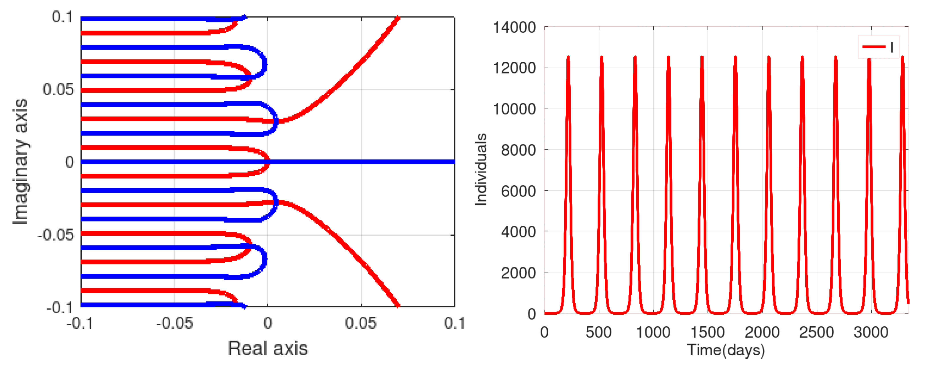
3.2. Stability of the Stationary Solution

Equation (3), linearized about the stationary solution, which is obtained by setting $J\left(t\right)=J_s+ϵe^{\lambda t}$ and keeping the first-order terms with respect to $ϵ$, has the following form:

$$v\left(t\right)=-a_1{\int }_{t-{\tau }_1-{\tau }_2}^{t}v\left(s\right)ds+a_2{\int }_{t-{\tau }_1}^{t}v\left(s\right)ds,$$

(7)

where

$$a_1=\frac{\beta }{N}\left(I_0+\frac{N}{\beta }\frac{\beta {\tau }_1-1}{{\tau }_1+{\tau }_2}\right),a_2=\frac{\beta }{N}\left(S_0-\frac{N}{\beta {\tau }_1}(\beta {\tau }_1-1)\right).$$

(8)

Set $v\left(t\right)=e^{\lambda t}$. Then, from Equation (7), we obtain:

$$\lambda =-a_1(1-e^{-({\tau }_1+{\tau }_2)\lambda })+a_2(1-e^{-{\tau }_1\lambda }).$$

(9)

Clearly, $\lambda =0$ is a solution of Equation (9). We will study the existence of solutions of this equation with a positive real part, which determines the loss of stability of the stationary solution. In order to simplify this analysis, we set $I_0=0,S_0=N$ in (8).

Lemma 1.

If ${\Re }_0>1$ and $J_s>0$, then Equation (9) does not have nontrivial positive real solutions.

Proof 1.

Let us denote the right-hand side of Equation (9) by $F\left(x\right)$,

$$F\left(x\right)=-a_1(1-e^{-({\tau }_1+{\tau }_2)x})+a_2(1-e^{-{\tau }_{1}x}).$$

(10)

Then,

$$F^{\prime }\left(0\right)=-a_1({\tau }_1+{\tau }_2)+a_2{\tau }_1=\frac{\beta }{N}[S_0{\tau }_1-({\tau }_1+{\tau }_2)(I_0+2{\tau }_1{J}_s)].$$

If we assume that $I_0<<{\tau }_1{J}_s$, then:

$$F^{\prime }\left(0\right)=\frac{\beta }{N}{S}_0{\tau }_1-\frac{2\beta }{N}{\tau }_1{J}_s({\tau }_1+{\tau }_2)$$

(11)

Note that $li{m}_{x\to -\infty }F\left(x\right)=\infty$, $li{m}_{x\to \infty }F\left(x\right)=a_2-a_1$,

$$F^{\prime }\left(x\right)=-a_1({\tau }_1+{\tau }_2)e^{-({\tau }_1+{\tau }_2)x}+a_2{\tau }_1{e}^{-{\tau }_{1}x}.$$

Next,

$$F^{\prime }\left(x\right)=0\Rightarrow x=\frac{-1}{{\tau }_2}ln\frac{a_2{\tau }_1}{a_1({\tau }_1+{\tau }_2)}=x_0$$

and

$$F^{\prime }\left(0\right)<0\iff 0<a_2{\tau }_1<a_1({\tau }_1+{\tau }_2)\iff x_0>0.$$

Let us prove that $0<F^{\prime }\left(x\right)<1$ for $x_0<x$. We note that $F^{\prime }\left(x_0\right)=0$, $li{m}_{x\to \infty }{F}^{\prime }\left(x\right)=0$, and

$$F^{″}\left(x\right)=a_1{({\tau }_1+{\tau }_2)}^2{e}^{-({\tau }_1+{\tau }_2)x}-a_2{\tau }_1^2{e}^{-{\tau }_{1}x}.$$

Since

$$F^{″}\left(x\right)=0\Rightarrow x=\frac{-2}{{\tau }_2}ln\frac{a_2{\tau }_1}{a_1({\tau }_1+{\tau }_2)}=x_1(=2x_0),$$

then

$$F^{\prime }\left(x_1\right)={\left(\frac{a_2{\tau }_1}{a_1({\tau }_1+{\tau }_2)}\right)}^{\frac{2{\tau }_1}{{\tau }_2}}{a}_2{\tau }_1\left(1-\frac{a_2{\tau }_1}{a_1({\tau }_1+{\tau }_2)}\right)<1.$$

Hence, Equation (9) does not have positive solutions for $F^{\prime }\left(0\right)<0$.

On the other hand,

$$F^{\prime }\left(0\right)>0\iff a_2{\tau }_1>a_1({\tau }_1+{\tau }_2)>0\iff x_0<0.$$

Since $0<a_1({\tau }_1+{\tau }_2)<a_2{\tau }_1<1$, then $0<F^{\prime }\left(x\right)<1$ for $[0,\infty )$, and Equation (9) does not have any positive solutions. The lemma is proven. □

Lemma 2.

If ${\Re }_0>1$ and $J_s=0$, then Equation (9) has exactly one positive real solution. If ${\Re }_0<1$, then this equation has only negative real solutions.

Proof  

For $J_s=0$, and assuming that $I_0=0$, $S_0=N$, we have $a_1=0$ and $a_2=\beta$. The function F defined in the previous lemma becomes $F\left(x\right)=\beta (1-e^{-{\tau }_{1}x}).$ Therefore,

$$F^{\prime }\left(x\right)=\beta {\tau }_1{e}^{-{\tau }_{1}x}={\Re }_0{e}^{-{\tau }_{1}x}>0.$$

Let us note that $F\left(0\right)=0$ and $F^{\prime }\left(0\right)={\Re }_0$. Thus, Equation (9) has exactly one positive real solution for ${\Re }_0>1$. If ${\Re }_0<1$, then this equation has only negative real solutions. □

Theorem 1.

Suppose that $I_0=0$ and $S_0=N$ in (8). If ${\Re }_0>1$, then Equation (9) has a pure imaginary solution y for any positive ${\tau }_1$ and ${\tau }_2$.

Proof  

Set $\lambda =x+iy$ in Equation (9). Then, we obtain:

$$x=a_2-a_1+a_1{e}^{-({\tau }_1+{\tau }_2)x}cos\left(({\tau }_1+{\tau }_2)y\right)-a_2{e}^{-{\tau }_{1}x}cos\left({\tau }_{1}y\right),$$

(12)

$$y=-a_1{e}^{-({\tau }_1+{\tau }_2)x}sin\left(({\tau }_1+{\tau }_2)y\right)+a_2{e}^{-{\tau }_{1}x}sin\left({\tau }_{1}y\right).$$

(13)

For $I_0=0$ and $S_0=N$ in (8), we have $a_1=\frac{\beta {\tau }_1-1}{{\tau }_1+{\tau }_2}=\frac{{\Re }_0-1}{{\tau }_1+{\tau }_2},a_2=\frac{1}{{\tau }_1}$. Substituting $x=0$ in (12) we achieve:

$$a_1=a_2\frac{1-cos\left({\tau }_{1}y\right)}{1-cos\left(({\tau }_1+{\tau }_2)y\right)},y\ne \frac{2\pi }{{\tau }_1+{\tau }_2}k,k\in \mathbb{Z}.$$

(14)

Hence, $a_1\ge 0$. From (13), we obtain

$$y=\frac{1}{{\tau }_1}\left(-\frac{1-cos\left({\tau }_{1}y\right)}{1-cos\left(({\tau }_1+{\tau }_2)y\right)}sin\left(({\tau }_1+{\tau }_2)y\right)+sin\left({\tau }_{1}y\right)\right).$$

(15)

Consider the function

$$f\left(y\right)=\frac{1}{{\tau }_1}\left(-\frac{1-cos\left({\tau }_{1}y\right)}{1-cos\left(({\tau }_1+{\tau }_2)y\right)}sin\left(({\tau }_1+{\tau }_2)y\right)+sin\left({\tau }_{1}y\right)\right)$$

on the interval $(0,\frac{2\pi }{{\tau }_1+{\tau }_2})$. We have

$$\underset{y\to \frac{2\pi }{{\tau }_1+{\tau }_2}}{lim}f\left(y\right)=\infty ,\underset{y\to 0}{lim}f\left(y\right)=0.$$

Furthermore,

$$f^{\prime }\left(y\right)=-sin\left({\tau }_{1}y\right)\frac{cos\left(\frac{{\tau }_1+{\tau }_2}{2}y\right)}{sin\left(\frac{{\tau }_1+{\tau }_2}{2}y\right)}+\left(1+\frac{{\tau }_2}{{\tau }_1}\right)\frac{si{n}^2\left(\frac{{\tau }_1}{2}y\right)}{si{n}^2\left(\frac{{\tau }_1+{\tau }_2}{2}y\right)}+cos\left({\tau }_{1}y\right).$$

It can be directly verified that $0<f^{\prime }\left(0\right)\approx \frac{{\tau }_2}{{\tau }_1+{\tau }_2}<1$. Therefore, the equation $y=f\left(y\right)$ has a nonzero solution within this interval.

We note that $1-cos\left({\tau }_{1}y\right)>0$ for the solution y. Indeed, otherwise, the only solution for Equation (15) is $y=0$. Hence, $a_1>0$ and ${\Re }_0>1$. The theorem is proved. □

Summarizing the results of this section, we conclude that the stationary solution $J_s=0$ loses its stability for ${\Re }_0>1$, and another stationary solution $J_s>0$ appears. Next, there exists a critical value ${\Re }_0={\Re }_c>1$ for which the oscillatory instability of the positive stationary solution occurs. Figure 1 (left) shows zero lines of the real and imaginary parts of the characteristic equation. They intersect in the positive half-plane, providing the existence of a pair of complex conjugate eigenvalues with a positive real part. The right panel of this figure illustrates the oscillations in direct numerical simulations of system (1). Note that the period of oscillations corresponds to the imaginary part of the eigenvalues for the values of parameters close to the stability boundary.

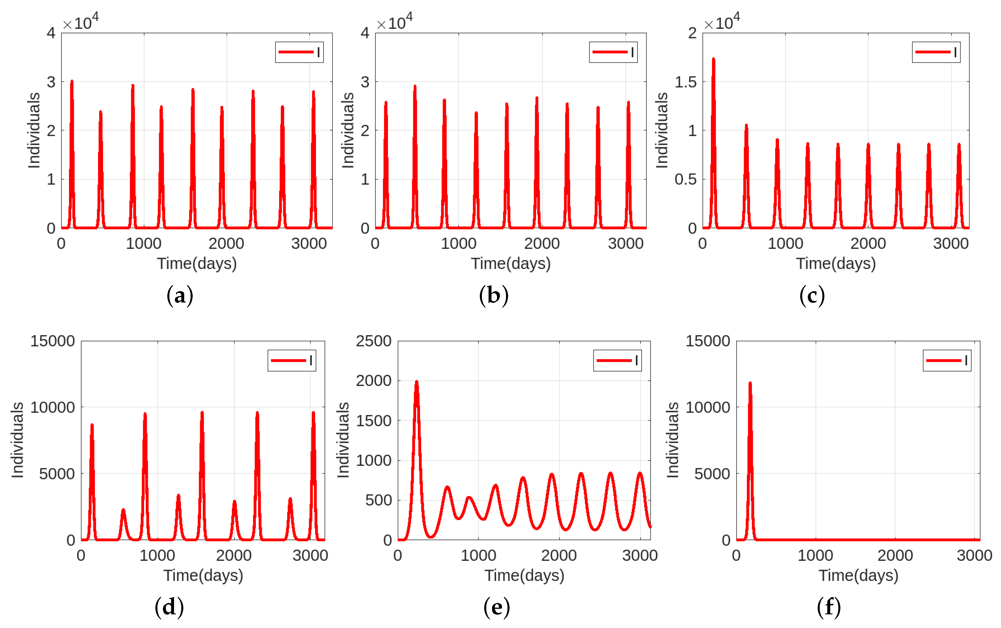
3.3. Numerical Simulations

In this section, we present some numerical simulations to verify the effect of disease transmission rate $\beta$, disease duration ${\tau }_1$ and the period of immunity waning ${\tau }_2$ on the amplitude and the period of the outbreaks for model (1) without vaccination. Figure 2 shows that increasing $\beta$ while keeping ${\tau }_1$ and ${\tau }_2$ fixed, increases the amplitude and decreases the period of outbreaks in the model (1) without vaccination. The amplitude becomes larger with the increase in disease duration ${\tau }_1$. On the other hand, the period of outbreaks decreases with the increase in the disease transmission rate $\beta$. Furthermore, the period approaches the sum of disease duration and period of natural immunity for large values of the disease transmission rate, ${lim}_{\beta \to \infty }T(\beta ,{\tau }_1,{\tau }_2)={\tau }_1+{\tau }_2$, where T is the period of outbreaks. On the other hand, the amplitude of outbreaks approaches the total size of the population for large values of $\beta$.

4. Epidemic Dynamics with Vaccination

We now study the influence of vaccination on the dynamics of epidemic progression. Figure 3 shows the dependence of these dynamics on the value of parameter $k_0$, characterizing the intensity of vaccination. The interaction of intrinsic oscillations with an imposed periodicity of vaccination results in more complex dynamics. For small values of $k_0$, the period of oscillations is the same as without vaccination, while the amplitude slightly oscillates. With the increase in this parameter, the oscillations become aperiodic, the time interval between them increases, and the variation of the amplitude of oscillations becomes more important. As such, in Figure 3b, there are modulated oscillations with an approximately constant period; in panel (c), the amplitude stabilizes to a smaller value with an increased period of oscillations. The next figure (d) manifests a double periodicity, and in (e), some of the epidemic outbreaks are almost suppressed. Finally, for large $k_0$ values, we observe periodic oscillations with an increased period, equalling twice the period of vaccination.

The average number of infected individuals $L_1=\frac{1}{n}{\int }_0^{nT}I\left(t\right)dt$ decreases with the increase in $k_0$ (Figure 4) and stabilizes to a constant for sufficiently large values of this parameter. Indeed, a further increase in this parameter does not practically influence the number of vaccinated individuals, which reaches its maximum. Parameter $\gamma$ characterizes the duration of vaccination. Under the increase in this parameter, the average number of infected decreases. If $\gamma$ is sufficiently large, the epidemic outbreaks are completely suppressed.

Figure 5 displays the effect of ${\tau }_3$ on the amplitude of the outbreaks. It shows that increasing the duration of vaccination immunity decreases the amplitude of the outbreaks. The interaction of intrinsic and imposed oscillations can lead to modulated oscillations. The period of epidemic outbreaks remains approximately constant. For sufficiently large values of ${\tau }_3$, the outbreaks disappear after the first one.

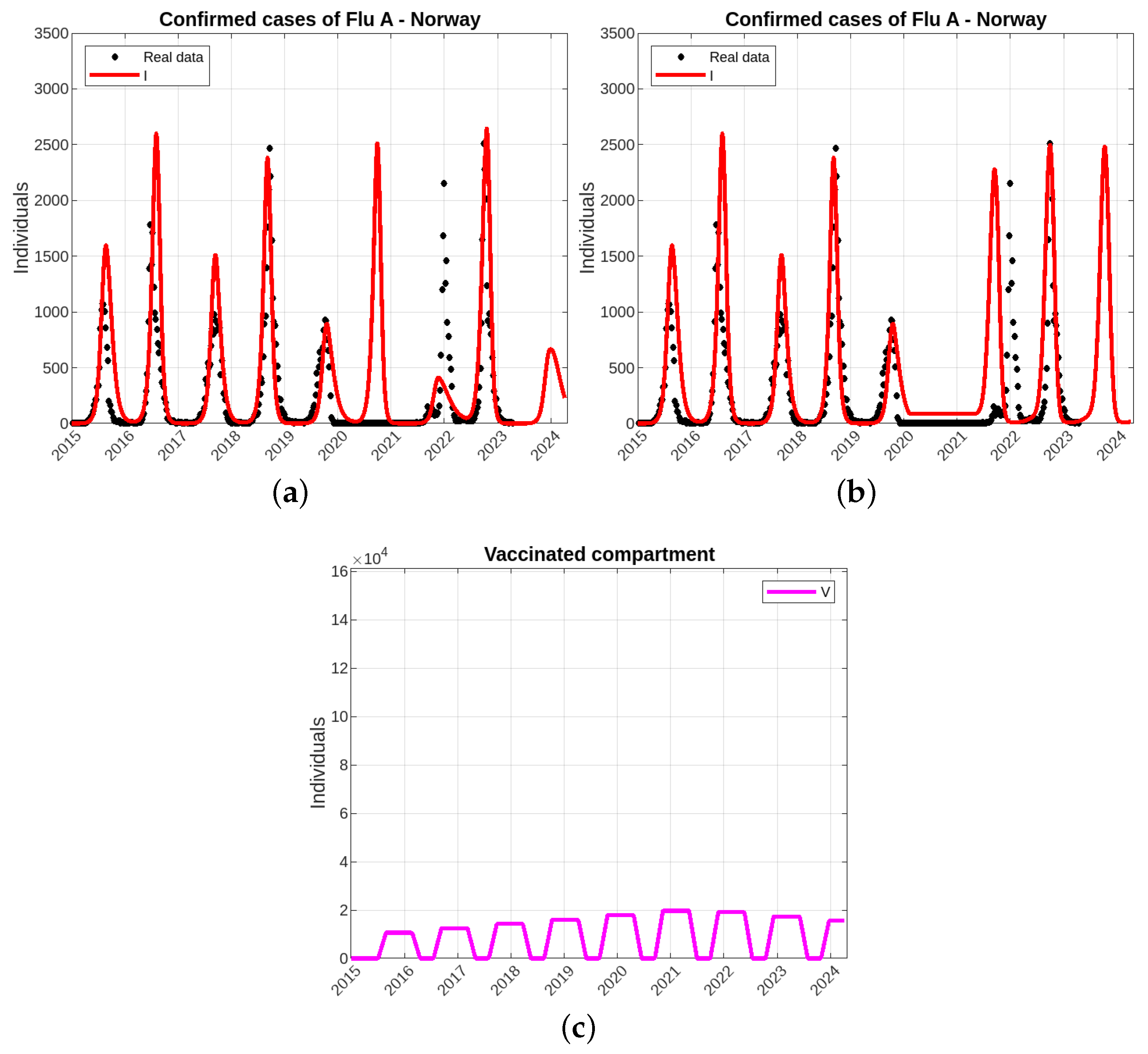
Modeling of Influenza A Epidemics

We now compare modeling results with the data on the Influenza A epidemic in Norway, chosen as example. Let us recall that disease duration in the case of influenza is about one week [42]. The influenza vaccine’s effectiveness starts to wane after five or six months [43]. The number of vaccine doses in Norway (2015–2023) is given in [44]. It increased until 2022, then it started to decrease, as represented in Figure 6c. Modulated aperiodic oscillations of epidemic outbreaks are well described by the model between 2015 and 2020.

Dynamics of Influenza A epidemics were perturbed in 2021 by the COVID-19 pandemic because of all measures adopted to restrain the propagation of the SARS-CoV-2 infection (social distancing, masks, etc.). As such, the model predicted a large epidemic peak in 2021 (Figure 6a), but this peak is absent in the data. On the other hand, the model predicted a small peak in 2022, while it is essentially larger in the data. The model and the data present similar results in 2023.

In order to take into account the measures of social distancing, we consider time-dependent disease transmission rate $\beta \left(t\right)$ and set it to zero in 2021: $\beta \left(t\right)=1.44$ for $t\le 254$, 0 for $255\le t\le 307$, and $1.54$ for $t\ge 308$ (time here is given in weeks, starting from 2015). The vaccination rate is given by the function

$$k\left(t\right)=(at+k_0)H(\gamma +sin({\gamma }_0+\frac{2\pi t}{T})),$$

(16)

where the factor $(at+k_0)$ is used to describe the variation of the vaccination rate according to the data. Note that the annual number of doses in the model is calculated with the integral $N_{doses}={\int }_0^{T}U\left(t\right)dt$. It is re-scaled to the total population in agreement with the data.

The results of modeling are shown in Figure 6b. There is no epidemic outbreak in 2021 since the disease transmission rate is zero. The outbreak in 2022 has the same maximum as in the data, but it occurs in the model slightly earlier. The time of its emergence can be controlled by the duration of the time interval where $\beta \left(t\right)=0$. As before, the data and modeling present similar results in 2023. The model prediction for 2024 changes; it can be expected that the measures adopted against the coronavirus epidemic will increase the influenza outbreak.

It is interesting to note that the value of $\beta$ slightly increases in Figure 6b after the COVID-19 epidemic. It can be related to an increased social activity after the imposed lockdowns.

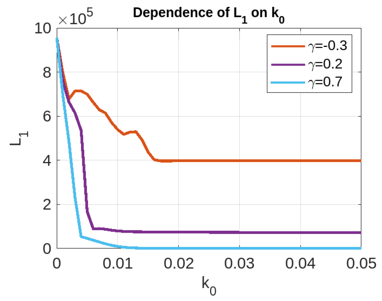
5. Optimal Control Problem

The control function $k\left(t\right)$ of vaccination is a T-periodic function. It is chosen in such a way that each year, there is only one time interval when people are vaccinated (Figure 7c). In the example of numerical simulations in Figure 7, the solution of the initial value problem associated to (1) rapidly approaches the periodic solution (Figure 7a) with slowly increasing amplitude of outbreaks (Figure 7b).

We consider the cost function as an averaged cost with respect to n periods:

$${\mathcal{L}}_n=\frac{1}{n}{\int }_0^{nT}(d_{0}I\left(t\right)+c_{0}k\left(t\right)\mathrm{sign}\left(S\left(t\right)\right)N)dt,$$

where $n\in \mathbb{N}$, $d_0$ is the social cost per infected individual and $c_0$ is the cost per vaccine dose and side effects. If $n\to +\infty$, ${\mathcal{L}}_n$ converges to the cost for one period of time, corresponding to the periodic solution of (1). If we normalize $d_0$, we can obtain the cost function

$$L=\frac{1}{n}{\int }_0^{nT}(I\left(t\right)+ck\left(t\right)\mathrm{sign}\left(S\left(t\right)\right)N)dt,$$

(17)

where c is a positive constant.

Our goal is to minimize $L(\gamma ,{\gamma }_0)$, where $\gamma \in [-1,1],{\gamma }_0\in [0,2\pi ]$. Figure 7d shows the cost function depending on these parameters. Its minimum is reached inside the domain for some particular values of $\gamma$ and ${\gamma }_0$. Figure 8 shows the cost function for different values of the parameter c, which determines the cost of vaccination. For a small c, L decreases as a function of $\gamma$, that is, with the increase in vaccination, and it is practically independent of ${\gamma }_0$, characterizing the beginning of the vaccination campaign. The minimization of L in this case occurs for the maximal vaccination. The internal local minimum of L appears for larger values of c. This minimum becomes global for sufficiently large vaccination costs (Figure 8d). In this case, the optimal vaccination strategy consists of an appropriate choice of the intensity and timing of vaccination.

We note that a similar approach can be used for several vaccinations per year. If we intend to vaccinate at most twice a year, then the control to be considered has the following form

$$k\left(t\right)=k_{0}H(\gamma +sin({\gamma }_0+\frac{2\pi t}{T}))H(\tilde{\gamma }+sin({\tilde{\gamma }}_0+\frac{2\pi t}{T})),$$

(18)

where $\gamma ,\tilde{\gamma }\in [-1,1],{\gamma }_0,{\tilde{\gamma }}_0\in [0,2\pi ]$. The structure of the control is more complicated but still simple, and numerical tests will be conclusive. The optimal control will be a quadruple $({\gamma }^{*},{\gamma }_0^{*},{\tilde{\gamma }}^{*},{\tilde{\gamma }}_0^{*})$, which represents the solution of the optimal control problem that results in the minimal cost of vaccination process. A similar approach may be used if more than two vaccinations per year are considered.

6. Discussion

In this work, we propose an epidemiological model based on delay differential equations with three time delays, representing the disease duration, the period of natural immunity, and the period of vaccine immunity. This work continues the previous studies [28,29,30], taking into account vaccination and vaccination control.

The reduction in the delay model to an integral equation allows us to study stationary solutions of this model and their stability. A positive stationary solution appears for the basic reproduction number larger than 1. It loses its stability and leads to periodic oscillations if the basic reproduction number exceeds some critical value. We determine this critical value and the period of emerging oscillations.

Numerical simulations display possible effects of the parameters on the amplitude and the periodicity of outbreaks. For instance, an increase in the disease transmission rate increases the amplitude and decreases the period of the outbreaks. For a large $\beta$ value, the period of outbreaks approaches the sum of disease duration and the period of natural immunity in the model without vaccination.

Periodic vaccination changes epidemic dynamics, resulting in modulated oscillations and influencing the period of oscillations. The vaccination rate and immunity duration affect the outbreaks in terms of amplitude and periodicity with various patterns.

A comparison with the epidemiological data on Influenza A in Norway shows that the model provides appropriate results in spite of the complexity of oscillations. It is interesting to note that the COVID-19 pandemic changed the dynamics of seasonal influenza epidemics beginning from 2021 due to the measures of social distancing. The model describes these new dynamics if we introduce time-dependent disease transmission rates.

An optimal control of vaccination enables us to minimize the cost of the epidemic. If the cost of vaccination is low, then the optimal cost is reached for the maximal vaccination level. If the vaccination cost is sufficiently high, it can influence the result of optimization. The minimum in this case can be reached for some particular choice of parameters, depending on the timing of the vaccination campaign.

This study has some limitations. First of all, discrete delays prescribe single values to the disease duration and immunity waning instead of some distributions. However, we have shown in previous works that such delay models provide a good approximation for the models with distributed delays [29]. Furthermore, we neglect exposed compartments and assume that the population is homogeneous with a fixed size. These questions and also some others, including different vaccination strategies, represent interesting open questions for forthcoming works. These modeling approaches can be used for data analyses from different countries and for different epidemics.

References

1. Fisher-Hoch, S.; Hutwagner, L. Opportunistic candidiasis: An epidemic of the 1980s. Clin. Infect. Dis. 1995, 21, 897–904. [Google Scholar] [CrossRef] [PubMed]
2. Chintu, C.; Athale, U.H.; Patil, P. Childhood cancers in Zambia before and after the HIV epidemic. Arch. Dis. Child. 1995, 73, 100–105. [Google Scholar] [CrossRef] [PubMed]
3. Anderson, R.M.; Fraser, C.; Ghani, A.C.; Donnelly, C.A.; Riley, S.; Ferguson, N.M.; Leung, G.M.; Lam, T.H.; Hedley, A.J. Epidemiology, transmission dynamics and control of SARS: The 2002–2003 epidemic. Philos. Trans. R. Soc. Lond. Ser. B Biol. Sci. 2004, 359, 1091–1105. [Google Scholar] [CrossRef] [PubMed]
4. Lam, W.; Zhong, N.; Tan, W. Overview on SARS in Asia and the world. Respirology 2003, 8, S2–S5. [Google Scholar] [CrossRef]
5. Chen, S.H.; Mallamace, F.; Mou, C.Y.; Broccio, M.; Corsaro, C.; Faraone, A.; Liu, L. The violation of the Stokes–Einstein relation in supercooled water. Proc. Natl. Acad. Sci. USA 2006, 103, 12974–12978. [Google Scholar] [CrossRef] [PubMed]
6. Kilpatrick, A.M.; Chmura, A.A.; Gibbons, D.W.; Fleischer, R.C.; Marra, P.P.; Daszak, P. Predicting the global spread of H5N1 avian influenza. Proc. Natl. Acad. Sci. USA 2006, 103, 19368–19373. [Google Scholar] [CrossRef] [PubMed]
7. Jain, S.; Kamimoto, L.; Bramley, A.M.; Schmitz, A.M.; Benoit, S.R.; Louie, J.; Sugerman, D.E.; Druckenmiller, J.K.; Ritger, K.A.; Chugh, R.; et al. Hospitalized patients with 2009 H1N1 influenza in the United States, April–June 2009. N. Engl. J. Med. 2009, 361, 1935–1944. [Google Scholar] [CrossRef]
8. Girard, M.P.; Tam, J.S.; Assossou, O.M.; Kieny, M.P. The 2009 A (H1N1) influenza virus pandemic: A review. Vaccine 2010, 28, 4895–4902. [Google Scholar] [CrossRef]
9. Briand, S.; Bertherat, E.; Cox, P.; Formenty, P.; Kieny, M.P.; Myhre, J.K.; Roth, C.; Shindo, N.; Dye, C. The international Ebola emergency. N. Engl. J. Med. 2014, 371, 1180–1183. [Google Scholar] [CrossRef]
10. Kreuels, B.; Wichmann, D.; Emmerich, P.; Schmidt-Chanasit, J.; de Heer, G.; Kluge, S.; Sow, A.; Renné, T.; Günther, S.; Lohse, A.W.; et al. A case of severe Ebola virus infection complicated by gram-negative septicemia. N. Engl. J. Med. 2014, 371, 2394–2401. [Google Scholar] [CrossRef]
11. Kapralov, M.; Khanna, S.; Sudan, M. Approximating matching size from random streams. In Proceedings of the Twenty-Fifth Annual ACM-SIAM Symposium on Discrete Algorithms, SIAM, Portland, OR, USA, 5–7 January 2014; pp. 734–751. [Google Scholar]
12. Almeida, R.; Qureshi, S. A fractional measles model having monotonic real statistical data for constant transmission rate of the disease. Fractal Fract. 2019, 3, 53. [Google Scholar] [CrossRef]
13. Sharma, S.; Volpert, V.; Banerjee, M. Extended SEIQR type model for COVID-19 epidemic and data analysis. MedRxiv 2020. [Google Scholar] [CrossRef]
14. Brauer, F.; Van den Driessche, P.; Wu, J.; Allen, L.J. Mathematical Epidemiology; Springer: Berlin/Heidelberg, Germany, 2008; Volume 1945. [Google Scholar]
15. d’Onofrio, A.; Banerjee, M.; Manfredi, P. Spatial behavioural responses to the spread of an infectious disease can suppress Turing and Turing–Hopf patterning of the disease. Phys. A Stat. Mech. Its Appl. 2020, 545, 123773. [Google Scholar] [CrossRef]
16. Sun, G.Q.; Jin, Z.; Liu, Q.X.; Li, L. Chaos induced by breakup of waves in a spatial epidemic model with nonlinear incidence rate. J. Stat. Mech. Theory Exp. 2008, 2008, P08011. [Google Scholar] [CrossRef]
17. Bichara, D.; Iggidr, A. Multi-patch and multi-group epidemic models: A new framework. J. Math. Biol. 2018, 77, 107–134. [Google Scholar] [CrossRef]
18. McCormack, R.K.; Allen, L.J. Multi-patch deterministic and stochastic models for wildlife diseases. J. Biol. Dyn. 2007, 1, 63–85. [Google Scholar] [CrossRef]
19. Elbasha, E.H.; Gumel, A.B. Vaccination and herd immunity thresholds in heterogeneous populations. J. Math. Biol. 2021, 83, 73. [Google Scholar] [CrossRef]
20. Aniţa, S.; Banerjee, M.; Ghosh, S.; Volpert, V. Vaccination in a two-group epidemic model. Appl. Math. Lett. 2021, 119, 107197. [Google Scholar] [CrossRef]
21. Faniran, T.S.; Ali, A.; Al-Hazmi, N.E.; Asamoah, J.K.K.; Nofal, T.A.; Adewole, M.O. New variant of SARS-CoV-2 dynamics with imperfect vaccine. Complexity 2022, 2022, 1062180. [Google Scholar] [CrossRef]
22. Ahmed, N.; Wei, Z.; Baleanu, D.; Rafiq, M.; Rehman, M. Spatio-temporal numerical modeling of reaction-diffusion measles epidemic system. Chaos Interdiscip. J. Nonlinear Sci. 2019, 29, 103101. [Google Scholar] [CrossRef]
23. Filipe, J.; Maule, M. Effects of dispersal mechanisms on spatio-temporal development of epidemics. J. Theor. Biol. 2004, 226, 125–141. [Google Scholar] [CrossRef]
24. Martcheva, M. An Introduction to Mathematical Epidemiology; Springer: Berlin/Heidelberg, Germany, 2015; Volume 61. [Google Scholar]
25. Brauer, F.; Castillo-Chavez, C.; Feng, Z. Mathematical Models in Epidemiology; Springer: Berlin/Heidelberg, Germany, 2019; Volume 32. [Google Scholar]
26. Hethcote, H.W. The mathematics of infectious diseases. SIAM Rev. 2000, 42, 599–653. [Google Scholar] [CrossRef]
27. Hurd, H.S.; Kaneene, J.B. The application of simulation models and systems analysis in epidemiology: A review. Prev. Vet. Med. 1993, 15, 81–99. [Google Scholar] [CrossRef]
28. Volpert, V.; Banerjee, M.; Petrovskii, S. On a quarantine model of coronavirus infection and data analysis. Math. Model. Nat. Phenom. 2020, 15, 24. [Google Scholar] [CrossRef]
29. Ghosh, S.; Volpert, V.; Banerjee, M. An epidemic model with time delay determined by the disease duration. Mathematics 2022, 10, 2561. [Google Scholar] [CrossRef]
30. Saade, M.; Ghosh, S.; Banerjee, M.; Volpert, V. An epidemic model with time delays determined by the infectivity and disease durations. Math. Biosci. Eng. 2023, 20, 12864–12888. [Google Scholar] [CrossRef]
31. Lenhart, S.; Workman, J.T. Optimal Control Applied to Biological Models; CRC Press: Boca Raton, FL, USA, 2007. [Google Scholar]
32. Schättler, H.; Ledzewicz, U. Optimal control for mathematical models of cancer therapies. In An Application of Geometric Methods; Springer: Berlin/Heidelberg, Germany, 2015. [Google Scholar]
33. Bolzoni, L.; Bonacini, E.; Soresina, C.; Groppi, M. Time-optimal control strategies in SIR epidemic models. Math. Biosci. 2017, 292, 86–96. [Google Scholar] [CrossRef]
34. Aniţa, S.; Capasso, V.; Scacchi, S. Controlling the spatial spread of a Xylella epidemic. Bull. Math. Biol. 2021, 83, 1–26. [Google Scholar] [CrossRef]
35. Aniţa, S.; Capasso, V.; Moşneagu, A.M. Regional control in optimal harvesting of population dynamics. Nonlinear Anal. Theory Methods Appl. 2016, 147, 191–212. [Google Scholar] [CrossRef]
36. Aniţa, S.; Capasso, V.; Kunze, H.; La Torre, D. Dynamics and optimal control in a spatially structured economic growth model with pollution diffusion and environmental taxation. Appl. Math. Lett. 2015, 42, 36–40. [Google Scholar] [CrossRef]
37. Aniţa, S.; Capasso, V.; Dimitriu, G. Regional control for a spatially structured malaria model. Math. Methods Appl. Sci. 2019, 42, 2909–2933. [Google Scholar] [CrossRef]
38. Aniţa, S.; Capasso, V. Reaction-diffusion systems in epidemiology. Ann. Alexandru Ioan Cuza Iaşi Math. 2017, 66, 171–196. [Google Scholar]
39. Jang, J.; Kwon, H.D.; Lee, J. Optimal control problem of an SIR reaction–diffusion model with inequality constraints. Math. Comput. Simul. 2020, 171, 136–151. [Google Scholar] [CrossRef]
40. Madubueze, C.E.; Dachollom, S.; Onwubuya, I.O. Controlling the spread of COVID-19: Optimal control analysis. Comput. Math. Methods Med. 2020, 2020, 6862516. [Google Scholar] [CrossRef] [PubMed]
41. Abbasi, Z.; Zamani, I.; Mehra, A.H.A.; Shafieirad, M.; Ibeas, A. Optimal control design of impulsive SQEIAR epidemic models with application to COVID-19. Chaos Solitons Fractals 2020, 139, 110054. [Google Scholar] [CrossRef]
42. Clinical Signs and Symptoms of Influenza. 2022. Available online: https://www.cdc.gov/flu/ (accessed on 28 August 2023).
43. Duda, K. How Long Does a Flu Shot Last? 2023. Available online: https://www.verywellhealth.com/ (accessed on 28 August 2023).
44. Hungnes, O.; Paulsen, T.H.; Rohringer, A.; Seppälä, E.M.; Tønnessen, R.; Bøås, H.; Dahl, J.; Fossum, E.; Stålcrantz, J.; Klüwer, B.; et al. Interim Influenza Virological and Epidemiological Season Report Prepared for the WHO Consultation on the Composition of Influenza Virus Vaccines for the Northern Hemisphere 2023/2024. 2023. Available online: https://hdl.handle.net/11250/3055881 (accessed on 28 August 2023).
45. Dattani, S.; Spooner, F.; Mathieu, E.; Ritchie, H.; Roser, M.; Influenza. Our World in Data 2023. Available online: https://ourworldindata.org/influenza (accessed on 28 August 2023).
46. World Health Organization. Respiratory Viruses Surveillance Country, Territory and Area Profiles, 2021; Technical Report; World Health Organization, Regional Office for Europe and European Centre: Geneva, Switzerland, 2022. [Google Scholar]
Figure 1. (Left): Solutions of Equations (12) (red curve) and (13) (blue curve) for the values of parameters N = 10 5 , β = 0.15 , τ 1 = 10 , τ 2 = 150 . The intersection of these curves gives the eigenvalues of the stationary points of the system (1). The eigenvalues with the positive real part are λ 1 , 2 0.0043 ± 0.027 i . The period of the oscillations is equal to | 2 π y | 227.26 . (Right): Numerical simulation for model (1) without vaccination for the values of the initial conditions N = 10 5 , S 0 = N 0.0001 , I 0 = 0.0001 , R 0 = 0 and parameters β = 0.15 , τ 1 = 10 ( 0 = 1.5 ) , τ 2 = 150 .
Mathematics 11 03770 g001
Figure 2. Dependence of the amplitude (a) and the period of outbreaks (b) for model (1) without vaccination on the disease transmission rate β for the initial conditions N = 10 5 , S 0 = N 0.0001 , I 0 = 0.0001 , R 0 = 0 , immunity waning τ 2 = 150 and disease duration τ 1 shown in each panel.
Mathematics 11 03770 g002
Figure 3. The size of the infected compartment for model (1) with the initial conditions N = 10 5 , S ( 0 ) = N 0.0001 , I ( 0 ) = 0.0001 , R ( 0 ) = V ( 0 ) = 0 , the parameters β = 0.2 , τ 1 = 10 , τ 2 = 150 , τ 3 = 180 , γ = 0.3 , γ 0 = 4 π 3 , T = 365 , and the values of k 0 as follows: (a) k 0 = 0.0001 , (b) k 0 = 0.001 , (c) k 0 = 0.002 , (d) k 0 = 0.006 , (e) k 0 = 0.01 , (f) k 0 = 0.05 .
Mathematics 11 03770 g003
Figure 4. The mean value of the infected compartment given by the integral L 1 = 1 n 0 n T I ( t ) d t as a function of k 0 for the initial conditions N = 10 5 , S 0 = N 0.0001 , I 0 = 0.0001 , R 0 = V 0 = 0 and parameters β = 0.2 , τ 1 = 10 , τ 2 = 150 , τ 3 = 180 , γ 0 = 4 π 3 , T = 365 , n = 10 , and the values of γ shown in the figure.
Mathematics 11 03770 g004
Figure 5. The size of the infected compartment for model (1) with the initial conditions N = 10 5 , S ( 0 ) = N 0.0001 , I ( 0 ) = 0.0001 , R ( 0 ) = V ( 0 ) = 0 , the parameters β = 0.2 , τ 1 = 10 , τ 2 = 150 , k 0 = 0.003 , γ = 0.3 , γ 0 = 4 π 3 , T = 365 , and the values of τ 3 as follows: (a) τ 3 = 210 ; (b) τ 3 = 240 ; (c) τ 3 = 270 ; (d) τ 3 = 300 ; (e) τ 3 = 360 ; (f) τ 3 = 420 .
Mathematics 11 03770 g005
Figure 6. Numerical simulations of model (1) describing the confirmed cases of Influenza A in Norway [45], for the initial conditions N = 5,379,475 × 0.03 , where 5379475 is the population of Norway and 0.03 is the percentage of covered population in the collecting data [46], S ( t ) = I ( t ) = R ( t ) = V ( t ) = 0 , t < 0 , S 0 = N 0.008 , I 0 = 0.008 , R 0 = V 0 = 0 , and parameters τ 1 = 0.8 , τ 2 = 24 , τ 3 = 32 , k ( t ) are given by (16), where a = 2.9 × 10 5 : t 307 , and a = 2.9 × 10 5 : t 308 , k 0 = 0.008 , T = 52 , γ = 0.9 , γ 0 = 6 π 5 . Time unit is week. (a) Constant value of β , (b) variable β taking into account COVID-19 (see the explanation in the text), (c) the number of vaccinated individuals with the annual number of doses corresponding to the data.
Mathematics 11 03770 g006
Figure 7. Numerical simulations of system (1). (a) Oscillations of four compartments are close to periodic with a slight increase in I ( t ) , (b) zoom in on I ( t ) , (c) vaccination rate, (d) cost function L depending on ( γ , γ 0 ) . Initial conditions N = 10 5 , S ( 0 ) = N 1 , I ( 0 ) = 1 , R ( 0 ) = V ( 0 ) = 0 , and parameters β = 0.2 , τ 1 = 10 , τ 2 = 150 , τ 3 = 180 , k 0 = 0.003 , T = 365 , n = 5 , c = 10 . The minimal value m i n ( L ) = 912,940.07 is reached for ( γ , γ 0 ) = ( 0.3 , 4 π 3 ) .
Mathematics 11 03770 g007
Figure 8. Dependence of L on γ and γ 0 for different vaccination costs c and for the following initial conditions N = 10 5 , S ( 0 ) = N 1 , I ( 0 ) = 1 , R ( 0 ) = V ( 0 ) = 0 , and parameters β = 0.2 , τ 1 = 10 , τ 2 = 150 , τ 3 = 180 , k 0 = 0.003 , T = 365 , n = 5 . (a) c = 1 ; (b) c = 5 ; (c) c = 7 ; (d) c = 10 .
Mathematics 11 03770 g008
Disclaimer/Publisher’s Note: The statements, opinions and data contained in all publications are solely those of the individual author(s) and contributor(s) and not of MDPI and/or the editor(s). MDPI and/or the editor(s) disclaim responsibility for any injury to people or property resulting from any ideas, methods, instructions or products referred to in the content.