An Inconvenient Truth about Forecast Combinations

Abstract

It is well-known that the weighted averages of two competing forecasts may reduce mean squared prediction errors (MSPE) and may also introduce certain inefficiencies. In this paper, we take an in-depth view of one particular type of inefficiency stemming from simple combination schemes: Mincer and Zarnowitz inefficiency or auto-inefficiency for short. Under mild assumptions, we show that linear convex forecast combinations are almost always auto-inefficient, and, therefore, greater reductions in MSPE are almost always possible. In particular, we show that the process of taking averages of forecasts may induce inefficiencies in the combination, even when individual forecasts are efficient. Furthermore, we show that the so-called “optimal weighted average” traditionally presented in the literature may indeed be inefficient as well. Finally, we illustrate our findings with simulations and an empirical application in the context of the combination of headline inflation forecasts for eight European economies. Overall, our results indicate that in situations in which a number of different forecasts are available, the combination of all of them should not be the last step taken in the search of forecast accuracy. Attempts to take advantage of potential inefficiencies stemming from the combination process should also be considered.

1. Introduction

Decision makers are quite often confronted with two or more forecasts for the same target variable. In this scenario, [1] identifies two possible different strategies: the search for the best possible single forecasting method and the search for the best possible combination of the available forecasts. This last strategy has received a lot of attention in the literature since the seminal work of [2]. In their article, the authors combine two sets of forecasts coming from airline passenger data. They conclude that a composite forecast may display fewer mean squared prediction errors (MSPE) than either of the single original projections.

Even when the superior predictive ability of one forecast over another is suspected, one could test for forecast encompassing. Refs. [3,4] claim that the superior accuracy of one forecast over another does not necessarily mean that the inferior forecast is useless. It could be the case that the superior forecast could benefit from using some of the information contained in the outperformed forecast. Granger and Newbold consider the possibility that an average of the superior and inferior forecasts may yield a new and more accurate forecast. When this is not possible, it is said that the superior forecast is not only more accurate than the outperformed forecast but also encompasses it (see [5,6]).

Since 1969, a number of different papers have been written on topics directly or indirectly related to the combination of forecasts. A sample of the influential work from the next two decades includes [7,8,9,10]. More recent papers are also published on the topic including, for instance, [11,12,13,14,15,16,17,18,19,20,21,22].

Despite the huge variety of combination methods available in the literature, two particular families of combination strategies have attracted special attention. Using the terms in [10], these two families are known as the variance–covariance method of [2] and the regression method, introduced by [8]. Broadly speaking, the first approach generates the combined forecast as a weighted average of the pool of single individual forecasts. Notice that this weighted average does not need to be convex. The latter approach is one in which the combining weights are obtained as the coefficient estimates of a regression between the target variable and the set of available individual forecasts. Figure 1 depicts the general situation that faces a decision maker confronted with two or more forecasts for the same target variable.

In general terms, the combination of forecasts is reported as a successful strategy to improve forecast accuracy. Ref. [1] shows an interesting table in which the simple average of several methods outperforms either of the individual forecasts available for US inflation. This is just one example of a pattern that the literature has been exploring so far. More empirical examples of the good behavior of combination schemes are found, for instance, in [7,17,23,24,25], just to name a few.

Different theoretical approaches aim at explaining the success of combination strategies. Given a set of forecasts and a loss function, the optimal combination could be found as the solution of an optimization problem looking for weights to minimize the expected loss. In many applications, such an optimization problem is well-defined and leads to non-trivial optimal weights, ensuring reductions in the loss function or, in other words, ensuring combination gains. Ref. [26] provides an interesting summary of the different environments in which combination gains are possible.

Despite these theoretical efforts, some questions are still unresolved. For instance, part of the relevant literature investigates what is known as the “Combination Puzzle“, which refers to the fact that simple combination schemes, like an arithmetic average, frequently outperform more complex and theoretically optimal combination rules. See, for instance, [27], for a discussion about this puzzle. More generally, as suggested by [15], the best way to build combination weights is still a matter of open debate.

While it is clear that combination gains may exist in a number of applications, part of the literature analyzes the efficiency of some combination strategies. For instance, ref. [10] indicates that the regression approach is a combination scheme that leaves room for improvement due to the autocorrelation in the residuals that is inherent to this combination method. Refs. [10,26] also mention that the Bates and Granger approach is potentially inefficient due to the introduction of the constraint of the coefficients summing to unity. The extent to which these inefficiencies are indeed relevant requires a case-by-case analysis, yet it is our reading of the literature that the potential inefficiencies of forecast combinations are mostly overshadowed by the enthusiastic literature that mainly emphasizes the direct benefits of forecast combinations in boosting forecast accuracy.

The main objective of this paper is to show that linear convex forecast combinations are almost always auto-inefficient, and, therefore, greater reductions in MSPE are almost always possible. By auto-inefficiency, we refer to the notion of efficiency analyzed by [28]. Aside from showing that auto-inefficiency almost always emerges in forecast combinations, we prove two additional results: First, we show that the process of taking averages of forecasts may induce inefficiencies in the combination, even when the individual forecasts are efficient. Second, we show that the so-called “optimal weighted average”, which is traditionally presented in the literature, may indeed be inefficient as well.

Currently, the state of the art in forecast combinations is to explore new different weighting schemes to combine forecasts, and no attempt to take advantage of potential inefficiencies stemming from the combination process is carried out. Our contribution to the existing literature is to show that auto-inefficiencies are commonplace in forecast combinations, which opens an interesting avenue for future research: to find the best way to remove these inefficiencies to further improve forecast accuracy.

We focus on linear convex combinations because they are used by practitioners in many empirical applications. In particular, Consensus Economics reports individual forecasts and their simple averages. Furthermore, many simple linear convex combinations are considered to be very accurate, which is consistent with the aforementioned combination puzzle. In addition, these combination strategies allow for an interpretation of the combination as a consensus forecast. Finally, many of these linear convex combinations do not require previous knowledge of the target variable to construct the combined forecast, which is a clear advantage of simple methods compared to the [8] approach.

The rest of the paper is organized as follows. In Section 2, we set the econometric environment. Section 3 contains the main theoretical results and simulated examples. Section 4 illustrates our findings with an empirical application. Section 5 concludes and presents possible extensions for further research. Appendix A provides some additional theoretical and empirical results.

2. Econometric Environment

Let us consider $\left\{Y_t\right\}$ to be a stationary and ergodic time series process. We assume that at time t we want to forecast the random variable $Y_{t+h}$, which is equivalent to say that we look for an h-step ahead of the forecast for our target variable. We use the following notation: $Y_{\mathrm{t}}\left(h\right)$ represents a generic forecast for the target variable $Y_{t+h}$, which is built with the information available at time $t$. We assume that we have two forecasts available for the same target variable $Y_{t+h}$. We denote these forecasts as $Y_{1,\mathrm{t}}\left(h\right)$ and $Y_{2,\mathrm{t}}\left(h\right)$.

We further assume that the vector process

$${\left(\begin{array}{c}{Y}_{1,\mathrm{t}}\left(h\right)\\ Y_{2,\mathrm{t}}\left(h\right)\\ Y_{t+h}\end{array}\right)}_{3\times 1}$$

is weakly stationary and ergodic and has a positive definite variance–covariance matrix $V$.

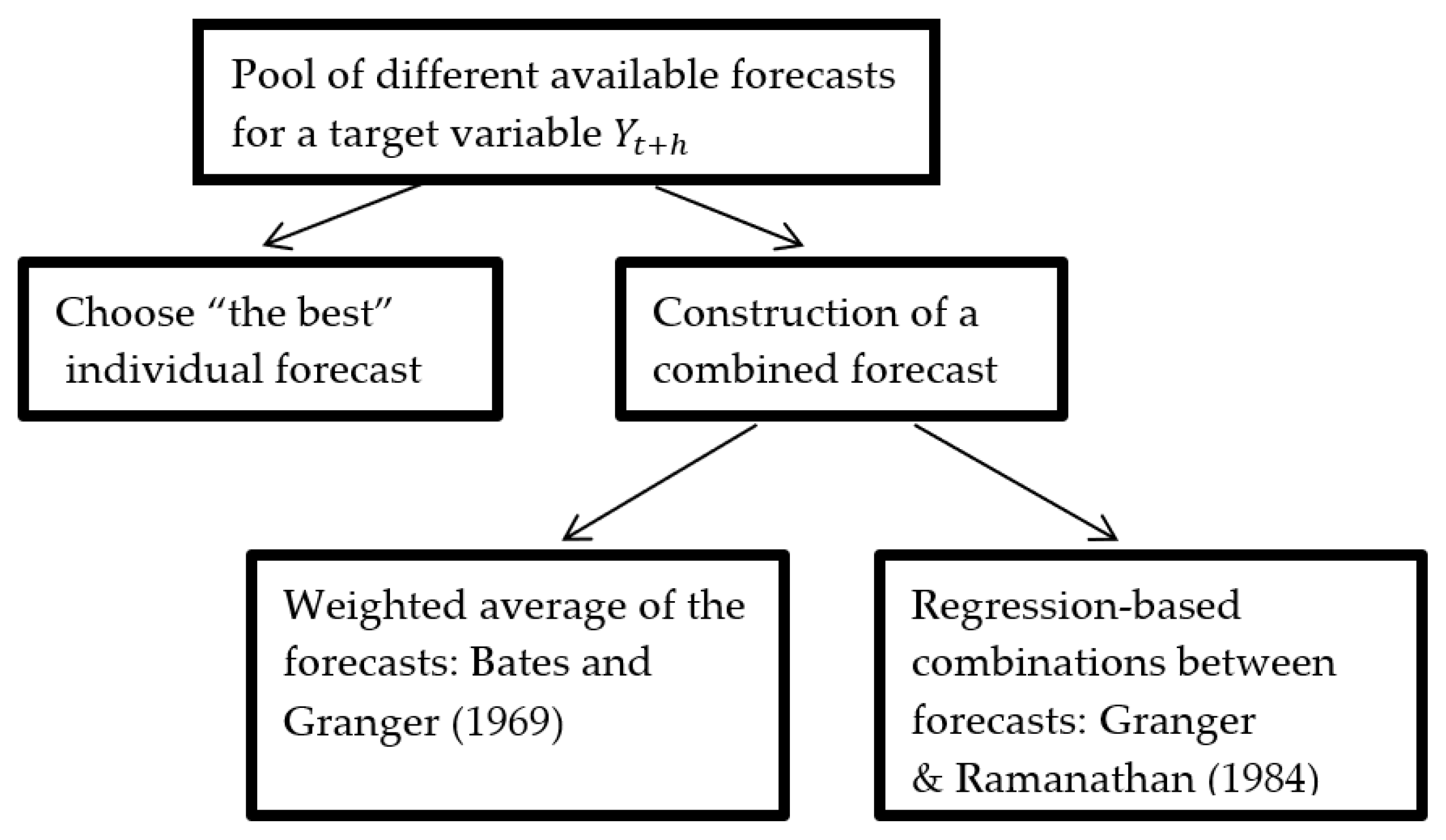
2.1. The Combined Forecast

Consider the following combination of forecasts

$$Y_t^c\left(h\right)=\lambda Y_{1,\mathrm{t}}\left(h\right)+\left(1-\lambda \right)Y_{2,\mathrm{t}}\left(h\right)=\lambda \left(Y_{1,\mathrm{t}}\left(h\right)-Y_{2,\mathrm{t}}\left(h\right)\right)+Y_{2,\mathrm{t}}\left(h\right)$$

(1)

$$\lambda \in [0,1]$$

where $Y_t^c\left(h\right)$ denotes the combined forecast. The corresponding forecast errors are

$$u_t^c\left(h\right)=\lambda u_{1,\mathrm{t}}\left(h\right)+\left(1-\lambda \right)u_{2,\mathrm{t}}\left(h\right)=\lambda \left(u_{1,\mathrm{t}}\left(h\right)-u_{2,\mathrm{t}}\left(h\right)\right)+u_{2,\mathrm{t}}\left(h\right)$$

(2)

where $u_{1,\mathrm{t}}(h)$ and $u_{2,\mathrm{t}}(h)$ represent the errors associated with forecasts $Y_{1,\mathrm{t}}(h)$ and $Y_{2,\mathrm{t}}\left(h\right)$, respectively:

$$u_{1,\mathrm{t}}\left(h\right)=Y_{t+h}-Y_{1,\mathrm{t}}\left(h\right),{ u}_{2,\mathrm{t}}\left(h\right)=Y_{t+h}-Y_{2,\mathrm{t}}\left(h\right)$$

(3)

We assume, without loss of generality, that the mean squared prediction errors ($MSPE$) of forecast 2 are as good as those of forecast 1, which is to say that

$$MSP{E}_2(h)\equiv E\left[u_{2,t}^2(h)\right]\le MSP{E}_1(h)\equiv E[u_{1,t}^2(h)]$$

(4)

When the combined forecast displays fewer $MSPE$ than forecasts $Y_{1,\mathrm{t}}(h)$ and $Y_{2,\mathrm{t}}(h)$ do, we follow [26] and say that combination gains (CG) do exist.

Proposition 1 shows the conditions for this to happen.

2.2. Combination Gains

Proposition 1.

If

$$E\left[u_{1,\mathrm{t}}(h)-u_{2,\mathrm{t}}(h)\right]\left[u_{2,\mathrm{t}}(h)\right]<0$$

(5)

then combination gains are possible for λ ∈ (0, 1).

Proof. 

Notice that

$$\begin{array}{c}E{\left[u_t^c(h)\right]}^2=E{\left[\lambda \left(u_{1,\mathrm{t}}\left(h\right)-u_{2,\mathrm{t}}\left(h\right)\right)+u_{2,\mathrm{t}}(h)\right]}^2\\ ={\lambda }^{2}E{\left[u_{1,\mathrm{t}}(h)-u_{2,\mathrm{t}}(h)\right]}^2+E{\left[u_{2,\mathrm{t}}(h)\right]}^2+2\lambda E\left[u_{1,\mathrm{t}}(h)-u_{2,\mathrm{t}}(h)\right][u_{2,\mathrm{t}}(h)]\end{array}$$

Therefore,

$$E{\left[u_t^c(h)\right]}^2-E{\left[u_{2,\mathrm{t}}(h)\right]}^2={\lambda }^{2}E{\left[u_{1,\mathrm{t}}(h)-u_{2,\mathrm{t}}(h)\right]}^2+2\lambda E\left[u_{1,\mathrm{t}}(h)-u_{2,\mathrm{t}}(h)\right][u_{2,\mathrm{t}}(h)]$$

(6)

As shown later, a direct implication of a positive definite variance–covariance matrix $V$ is that

$$E{\left[u_{1,\mathrm{t}}(h)-u_{2,\mathrm{t}}(h)\right]}^2=E{\left[Y_{1,\mathrm{t}}(h)-Y_{2,\mathrm{t}}(h)\right]}^2>0$$

With this, we can see that (6) is a strictly convex quadratic form with, at most, two different real roots. One of them is zero, which rules out the possibility of two complex roots. The other real root is

$${\lambda }_2^u=\frac{-2E\left[u_{1,\mathrm{t}}(h)-u_{2,\mathrm{t}}(h)\right][u_{2,\mathrm{t}}(h)]}{E{\left[u_{1,\mathrm{t}}\left(h\right)-u_{2,\mathrm{t}}\left(h\right)\right]}^2}>0$$

(7)

Univariate convex quadratic forms with a zero root must fall into one of the three cases depicted in Scheme 1. Given that ${\lambda }_2^u>0$, we are in a situation like that depicted with the blue line. Therefore, combination gains are achieved in the interval of

$$(0,{\lambda }_2^u)$$

which, in particular, ensures combination gains in, at least, a subset of the open set $(0, 1)$. □

Well acquainted with this analysis, [12] proposes testing the following null hypothesis of no encompassing

$$H_0:E\left[u_{1,\mathrm{t}}(h)-u_{2,\mathrm{t}}(h)\right]\left[u_{2,\mathrm{t}}\left(h\right)\right]=0$$

(8)

Under this null hypothesis, a combination of forecasts is not improving the accuracy because

$$E{\left[u_t^c(h)\right]}^2\ge E{\left[u_{2,\mathrm{t}}(h)\right]}^2 \forall \lambda \in R$$

(9)

and no combination gains are possible.

We are also interested in analyzing a particular property of forecasts that we call auto-efficiency.

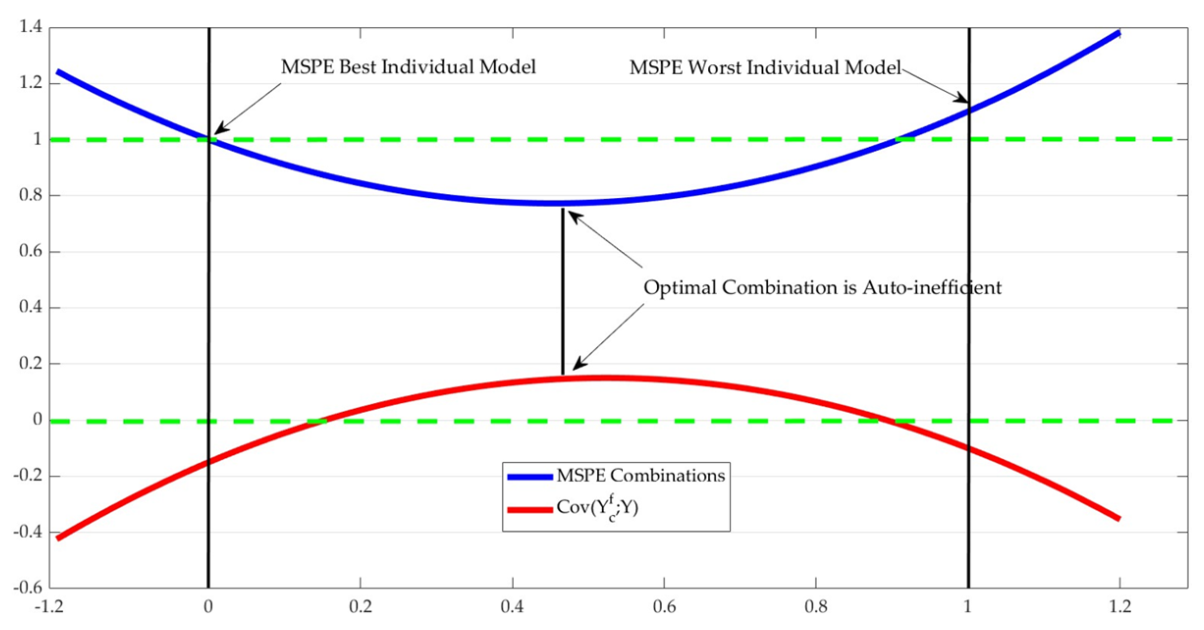
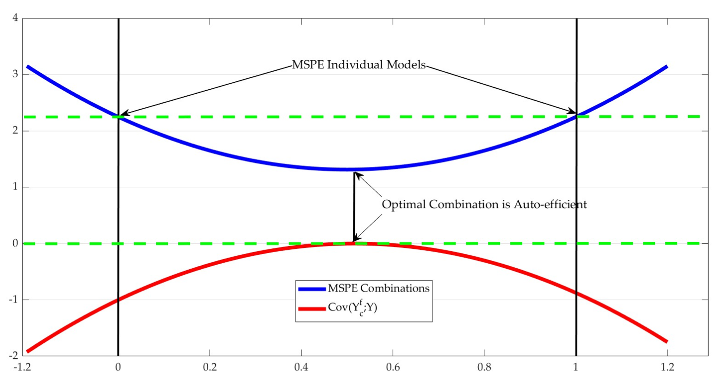
2.3. Auto-Efficiency

Definition 1.

Consider a target variable $Y_{t+h}$ and a forecast $Y_t^f(h)$. We say that the forecast $Y_t^f(h)$ is auto-efficient as long as

$$Cov\left(Y_{t+h}-Y_t^f(h),Y_t^f(h) \right)=0$$

(10)

 which, in the case of $Y_t^f(h)$ being unbiased, could be expressed as

$$E\left[Y_{t+h}-Y_t^f(h)\right]\left[Y_t^f(h)\right]=0$$

(11)

This last expression indicates that forecast errors are orthogonal to the forecast itself. If this condition does not hold true, we say that the forecast $Y_t^f(h)$ is auto-inefficient. In general, definitions in the same line are originally attributed to the early work of [28] and are called Minzer–Zarnowitz efficiency.

Notice that auto-efficiency is one of the conditions satisfied by optimal forecasts under quadratic loss. Furthermore, the notion of auto-efficiency is relevant for at least two reasons:

(1)

When forecasts are unbiased, auto-inefficiency compromises the inverse relationship between the MSPE and the explained variance of the forecast.

(2)

Violations of auto-efficiency, in theory, allow for a simple modification of the forecast $Y_t^f(h)$ to produce a new revised forecast with fewer MSPE than $Y_t^f(h)$.

Let us briefly explain the previous two points in more detail. The first point above relies on a remark made by [29]. Notice that

$$Y_{t+h}=Y_t^f(h)+u_t^f(h)$$

where $u_t^f\left(h\right)$ is the forecast error.

Therefore,

$$V\left(Y_{t+h}\right)=V\left(Y_t^f(h)\right)+2Cov\left(u_t^f(h),Y_t^f(h)\right)+V(u_t^f(h))$$

When forecasts are unbiased, we have that

$$E\left[Y_{t+h}\right]=E[Y_t^f(h)]$$

So

$$E\left(Y_{t+h}-Y_t^f(h)\right)=E\left(u_t^f(h)\right)=0$$

$$Cov\left(Y_t^f(h),u_t^f(h)\right)=E\left[Y_t^f(h)u_t^f(h)\right]$$

$$V\left(u_t^f(h)\right)=E{\left(u_t^f(h)\right)}^2$$

Therefore,

$$V\left(Y_{t+h}\right)=V\left(Y_t^f\left(h\right)\right)+2 E\left[Y_t^f\left(h\right)u_t^f\left(h\right)\right]+E{\left(u_t^f\left(h\right)\right)}^2$$

So, if auto-efficiency holds,

$$V\left(Y_{t+h}\right)=V\left(Y_t^f\left(h\right)\right)+MSPE(h)$$

(12)

$$MSPE(h)\equiv E{\left(u_t^f(h)\right)}^2$$

and there is an inverse relationship between $MSPE(h)$ and the “explained” variance of model $V\left(Y_t^f\left(h\right)\right)$. Nevertheless, if auto-efficiency does not hold, we can have reductions in $MSPE(h)$ that are associated with reductions in the “explained” variance of the model as well, which is counterintuitive.

Point (2) indicates that, when auto-inefficiency holds true, the forecast itself contains information that could be used to predict its own forecast errors. We could then build a linear model for the forecast errors as follows:

$$u_t^f(h)\equiv Y_{t+h}-Y_t^f\left(h\right)=\alpha +\beta Y_t^f\left(h\right)+u_t^{*}(h)$$

(13)

$$E{(u}_t^{*}(h))=E{(Y}_t^f\left(h\right)u_t^{*}(h))=0$$

(14)

which define the following coefficients:

$$\beta \equiv \frac{Cov\left(Y_t^f\left(h\right),u_t^f(h)\right)}{V\left(Y_t^f\left(h\right)\right)};\alpha \equiv E\left(u_t^f(h)\right)-\beta E\left(Y_t^f\left(h\right)\right)$$

(15)

We could build a revised forecast $Y_t^{fr}\left(h\right)$ as follows:

$$Y_t^{fr}\left(h\right)=\alpha +\left(1+\beta \right)Y_t^f\left(h\right)$$

$$Y_t^{fr}\left(h\right)=E\left(u_t^f(h)\right)-\beta E\left(Y_t^f\left(h\right)\right)+\left(1+\beta \right)\left(Y_t^f\left(h\right)\right)$$

$$Y_t^{fr}\left(h\right)=Y_t^f\left(h\right)+E\left(u_t^f(h)\right)+\beta \left(Y_t^f\left(h\right)-E\left(Y_t^f\left(h\right)\right)\right)$$

(16)

When forecasts are unbiased, we have $E\left(u_t^f(h)\right)=0$ and, consequently,

$$Y_t^{fr}\left(h\right)=Y_t^f\left(h\right)+\beta \left(Y_t^f\left(h\right)-E\left(Y_t^f\left(h\right)\right)\right)$$

(17)

Therefore, $\beta$ provides information regarding the need for shrinkage or an upscale adjustment in the term $\left(Y_t^f\left(h\right)-E\left(Y_t^f\left(h\right)\right)\right)$.

The new forecast error would be

$$\begin{array}{c}{Y}_{t+h}-Y_t^{fr}\left(h\right)=Y_{t+h}-\alpha -\left(1+\beta \right)Y_t^f\left(h\right)\\ =Y_{t+h}-Y_t^f\left(h\right)-\alpha -\beta Y_t^f\left(h\right)\\ =u_t^f(h)-\left(\alpha +\beta Y_t^f\left(h\right)\right)\\ =u_t^{*}(h)\end{array}$$

(18)

Interestingly,

$$E{\left[u_t^{*}(h)\right]}^2<E{\left[u_t^f(h)\right]}^2$$

(19)

This is so, as long as $\left(\alpha +\beta Y_t^f\left(h\right)\right)\ne 0$. In fact,

$$\begin{array}{c}E{\left[u_t^{*}(h)\right]}^2=E{\left[u_t^f(h)-\left(\alpha +\beta Y_t^f\left(h\right)\right)\right]}^2\\ =E{\left[u_t^f(h)\right]}^2+E{\left[\alpha +\beta Y_t^f\left(h\right)\right]}^2-2E[u_t^f(h)\left(\alpha +\beta Y_t^f\left(h\right)\right)]\\ =E{\left[u_t^f(h)\right]}^2+E{\left[\alpha +\beta Y_t^f\left(h\right)\right]}^2-2E\left[\left(\alpha +\beta Y_t^f\left(h\right)+u_t^{*}(h)\right)\left(\alpha +\beta Y_t^f\left(h\right)\right)\right]\\ =E{\left[u_t^f(h)\right]}^2+E{\left[\alpha +\beta Y_t^f\left(h\right)\right]}^2-2E{\left[\alpha +\beta Y_t^f\left(h\right)\right]}^2-2E\left[u_t^{*}(h)\left(\alpha +\beta Y_t^f\left(h\right)\right)\right]\\ =E{\left[u_t^f(h)\right]}^2-E{\left[\alpha +\beta Y_t^f\left(h\right)\right]}^2\end{array}$$

(20)

Notice that even if the original forecast is unbiased, we may have $\alpha \ne 0$. This is so because

$$\alpha \equiv E\left(u_t^f(h)\right)-\beta E\left(Y_t^f\left(h\right)\right)$$

So, in the unbiased case,

$$\alpha \equiv -\beta E\left(Y_t^f\left(h\right)\right)$$

(21)

And $\alpha$ may still be different from zero, due to the auto-inefficiency of $Y_t^f\left(h\right)$, as long as

$$E\left(Y_{t+h}\right)\ne 0$$

In the next subsection, we describe the assumptions that we need to obtain our main results.

2.4. Assumptions

We are interested in an environment characterized by

• One target variable $Y_{t+h}$.
• Two forecasts $Y_{1,\mathrm{t}}(h)$ and $Y_{2,\mathrm{t}}(h)$, such that

  $$MSP{E}_2(h)\equiv E{\left[u_{2,\mathrm{t}}(h)\right]}^2\le MSP{E}_1(h)\equiv E{\left[u_{1,\mathrm{t}}(h)\right]}^2$$

  (22)

  $$E\left[u_{1,\mathrm{t}}(h)\right]=E\left[u_{2,\mathrm{t}}(h)\right]=0$$

  (23)
• Combination gains do exist in a region of the open set (0, 1). In other words,

  $$E\left[u_{1,\mathrm{t}}(h)-u_{2,\mathrm{t}}(h)\right]\left[u_{2,\mathrm{t}}(h)\right]<0$$

  (24)
  We also make use of the following assumption.
• The following vector

  $${W_t=\left(\begin{array}{c}{Y}_{1,\mathrm{t}}\left(h\right)\\ Y_{2,\mathrm{t}}\left(h\right)\\ Y_{t+h}\end{array}\right)}_{3x1}$$

and is weakly stationary and ergodic, with a positive definite variance–covariance matrix, V. Notice that we have explicitly removed the horizon “h” from $W_t$. This is just to emphasize that the relevant sub index is t, as we are considering h as a fixed horizon relative to t.

From now on, we use a simpler notation. Let $\tilde{Y}=Y_{t+h}$. This is our target variable to forecast. We also drop the “t” subscript from $Y_{1,\mathrm{t}}\left(h\right)$, $Y_{2,\mathrm{t}}\left(h\right)$, and $Y_t^c\left(h\right)$ to further simplify the notation. We do the same with the corresponding forecast errors, so they look as follows:

$$u_1(h)=\tilde{Y}-Y_1(h),{ u}_2(h)=\tilde{Y}-Y_2(h)$$

$$u^c(h)=\lambda u_1(h)+\left(1-\lambda \right){ u}_2(h)=\lambda \left(u_1(h)-{ u}_2(h)\right)+{ u}_2(h)$$

Notice that a direct implication of a positive definite variance–covariance matrix V is that

$$E{\left[Y_1(h)-Y_2(h)\right]}^2>0$$

(25)

Otherwise, we would have

$$0=E{\left[Y_1(h)-Y_2(h)\right]}^2=V\left(Y_1(h)-Y_2(h)\right)+{\left[E\left(Y_1\left(h\right)-Y_2\left(h\right)\right)\right]}^2$$

(26)

and, due to the assumption of unbiased forecasts, we would have

$$V\left(Y_1(h)-Y_2(h)\right)=0$$

This means that

$$V\left(Y_1(h)\right)+V\left(Y_2(h)\right)=2Cov(Y_1(h),Y_2(h))$$

Let us consider $V_{12}$ to be defined as the variance covariance matrix of sub-vector

$${\left(\begin{array}{c}{Y}_1\left(h\right)\\ Y_2\left(h\right)\end{array}\right)}_{2x1}$$

Then, it has to be the case that $V_{12}$ is a positive definite matrix as well. Nevertheless

$$\left[\begin{array}{cc}1& -1\end{array}\right]V_{12}\left[\begin{array}{c}1\\ -1\end{array}\right]=V\left(Y_1(h)\right)-2Cov\left(Y_1(h),Y_2(h)\right)+V\left(Y_2(h)\right)=0$$

which is a contradiction to the fact that $V_{12}$ is positive and definite.

Remark 1.

Expression (25) is important. It says that $Y_1(h)$ and $Y_2(h)$ are not exactly the same probabilistic forecasts. They are distinct in a meaningful sense, so we combine forecasts embedding different information.

We have displayed the basic econometric framework and simplified notation that we are using in this paper. In the next section, we show the main results of the article.

3. Main Theoretical Results

One of the main points of this paper is to show that traditional weighted averages of forecasts are almost always auto-inefficient. In fact, the next proposition shows that the majority of forecast combinations with λ ∈ (0, 1) are auto-inefficient. Previous to that though, notice that with straightforward algebra the auto-efficiency of the combined forecast could be expressed in the following way:

$$\begin{array}{cc}\hfill E\left[Y^c\left(h\right)u^c\left(h\right)\right]=& -{\lambda }^{2}E{\left[Y_1\left(h\right)-Y_2\left(h\right)\right]}^2+\lambda E\left[Y_1\left(h\right)-Y_2\left(h\right)\right]\left[u_2\left(h\right)-Y_2\left(h\right)\right]\hfill \\ & +E\left[Y_2\left(h\right)u_2\left(h\right)\right]\hfill \end{array}$$

(27)

It would be also useful to express (27) as follows:

$$\begin{array}{cc}\hfill E\left[Y^c\left(h\right)u^c\left(h\right)\right]=& {\lambda }^{2}E\left[Y_1(h)u_1(h)\right]+{\left(1-\lambda \right)}^{2}E\left[Y_2(h)u_2(h)\right]\\ & +\lambda \left(1-\lambda \right)E\left[Y_1(h)u_2(h){+Y}_2(h)u_1(h)\right]\hfill \end{array}$$

(28)

The proofs of these expressions are in the Appendix A.

3.1. Auto-Inefficiency of Forecast Combinations

Proposition 2.

Let $\tilde{Y}$ denote a target variable and $Y_1\left(h\right), Y_2(h) denote$ two forecasts for $\tilde{Y}$, such that assumptions 1–4 hold true. Then, there are at most two different combinations ${\lambda }_1,{\lambda }_2\in (0,1)$, for which the combined forecast is auto-efficient.

Proof. 

Let us consider the expected value of the combined forecast times its forecast error:

$$E\left[Y^c\left(h\right)u^c\left(h\right)\right]=E\left[\lambda \left(Y_1\left(h\right)-Y_2(h)\right)+Y_2(h)\right][\lambda \left(u_1(h)-u_2(h)\right)+u_2(h)]$$

(29)

This expression defines the quadratic form in (27):

$$E\left[Y^c\left(h\right)u^c\left(h\right)\right]=-{\lambda }^{2}E{\left[Y_1\left(h\right)-Y_2(h)\right]}^2+\lambda E\left[Y_1\left(h\right)-Y_2(h)\right]\left[u_2(h)-Y_2(h)\right]+E\left[Y_2(h)u_2(h)\right]$$

Let us recall that we already showed that the following expression (25) holds true:

$$E{\left[Y_1\left(h\right)-Y_2(h)\right]}^2>0$$

This means that $E\left[Y^c\left(h\right)u^c\left(h\right)\right]$ is a strictly concave quadratic form and, of course, is different from the zero function. As a consequence, $E\left[Y^c\left(h\right)u^c\left(h\right)\right]$ has, at most, two real roots that may or may not lie within the (0,1) interval, so it may be the case that every single combination is auto-efficient. In any case, at most, two combinations are auto-efficient. □

Corollary 1.

Under Assumptions 1–4, if we further assume that both individual forecasts are auto-efficient, then any weighted average of the forecasts display a positive auto-inefficiency.

Proof. 

We already saw that

$$0<E{\left[Y_1\left(h\right)-Y_2(h)\right]}^2$$

Notice that

$$0<E{\left[Y_1\left(h\right)-Y_2(h)\right]}^2=E\left[Y_1\left(h\right)-Y_2(h)\right][u_2(h)-u_1(h)]$$

$$0<E{\left[Y_1\left(h\right)-Y_2(h)\right]}^2=E[Y_1\left(h\right)u_2(h)-Y_1\left(h\right)u_1(h)-Y_2(h)u_2(h)+Y_2(h)u_1(h)]$$

$$0<E{\left[Y_1\left(h\right)-Y_2(h)\right]}^2=E[Y_1\left(h\right)u_2(h)+Y_2(h)u_1(h)]$$

Using expression (27),

$$E\left[Y^c\left(h\right)u^c\left(h\right)\right]={\lambda }^{2}E\left[Y_1\left(h\right)u_1\left(h\right)\right]+{\left(1-\lambda \right)}^{2}E\left[Y_2\left(h\right)u_2\left(h\right)\right]+\lambda \left(1-\lambda \right)E\left[Y_1\left(h\right)u_2(h)+Y_2(h) u_1(h)\right]$$

Given that the two individual forecasts are auto-efficient,

$$E\left[Y_1\left(h\right)u_1(h)\right]=E\left[Y_2(h)u_2(h)\right]=0$$

so we have

$$E\left[Y^c\left(h\right)u^c\left(h\right)\right]=\left(1-\lambda \right)\lambda E\left[Y_1\left(h\right)u_2(h)+Y_2(h)u_1(h)\right]>0 \forall \lambda \in \left(0,1\right)$$

(30)

 □

Proposition 2 shows that most of the possible forecast combinations are auto-inefficient. The previous corollary shows a particular case ensuring that all possible combinations within (0, 1) are auto-inefficient, even if both individual forecasts are auto-efficient. This is important because disregarding this result may lead to incorrect conclusions when analyzing tests based upon aggregated information from surveys. The finding that a combination of forecasts is inefficient does not imply that individual forecasts share this property.

The next proposition provides more general conditions under which every single combination in (0, 1) is auto-inefficient.

Proposition 3.

For $\tilde{Y}$, $Y_1\left(h\right)$, and $Y_2(h)$, as in Proposition 2, let us assume that

$$E\left[Y_1\left(h\right)u_1(h)\right]\ge 0$$

(31)

$$E\left[Y_2(h)u_2(h)\right]\ge 0$$

(32)

Then, for every single combination $\lambda \in (0,1)$, the combined forecast displays auto-inefficiency.

Proof. 

Using

$$0<E{\left[Y_1\left(h\right)-Y_2(h)\right]}^2=E\left[Y_1\left(h\right)-Y_2(h)\right][u_2(h)-u_1(h)]$$

$$0<E{\left[Y_1\left(h\right)-Y_2(h)\right]}^2=E[Y_1\left(h\right)u_2(h)-Y_1\left(h\right)u_1(h)-Y_2(h)u_2(h)+Y_2(h)u_1(h)]$$

we obtain

$$0<E\left[Y_1\left(h\right)u_2(h)+Y_2(h)u_1(h)\right]-E[Y_1\left(h\right)u_1(h)+Y_2(h)u_2(h)]$$

Therefore,

$$E\left[Y_1\left(h\right)u_1(h)+Y_2(h)u_2(h)\right]<E[Y_1\left(h\right)u_2(h)+Y_2(h)u_1(h)]$$

But, because we are assuming that (31) and (32) hold true, we have that the left-hand-side in the previous inequality is greater than or equal to zero:

$$0\le E\left[Y_1\left(h\right)u_1\left(h\right)+Y_2\left(h\right)u_2\left(h\right)\right]<E[Y_1\left(h\right)u_2(h)+Y_2(h)u_1(h)]$$

Therefore,

$$0<E[Y_1\left(h\right)u_2(h)+Y_2(h)u_1(h)]$$

Again using expression (27),

$$E\left[Y^c\left(h\right)u^c\left(h\right)\right]={\lambda }^{2}E\left[Y_1\left(h\right)u_1(h)\right]+{\left(1-\lambda \right)}^{2}E\left[Y_2(h)u_2(h)\right]+\lambda \left(1-\lambda \right)E\left[Y_1\left(h\right)u_2(h)+Y_2(h)u_1(h)\right]$$

we conclude that

$$\begin{array}{c}E\left[Y^c\left(h\right)u^c\left(h\right)\right]={\lambda }^{2}E\left[Y_1\left(h\right)u_1\left(h\right)\right]+{\left(1-\lambda \right)}^{2}E\left[Y_2\left(h\right)u_2\left(h\right)\right]+\\ +\lambda \left(1-\lambda \right)E\left[Y_1\left(h\right)u_2(h)+Y_2(h)u_1(h)\right]>0 \forall \lambda \in (0,1)\end{array}$$

(33)

 □

It is important to remark that conditions (31) and (32) may be tested using simple tests or a strategy based on the “reality check” of [30], which is also used in [31].

The next proposition explores if, by any chance, the optimal forecast combination satisfies some special condition of auto-efficiency.

Proposition 4.

For $\tilde{Y}$, $Y_1\left(h\right)$, and $Y_2(h)$, as in Proposition 3, we can find a unique ${\lambda }^{*}\in (0,1)$ such that

$${\lambda }^{*}=Arg\underset{\lambda \in (0,1)}{\min }E{\left[\lambda u_1\left(h\right)+\left(1-\lambda \right)u_2\left(h\right)\right]}^2$$

For this ${\lambda }^{*}$, we also have

$$E\left[Y^c\left(h\right)u^c\left(h\right)\right]{|}_{{\lambda }^{*}}={\lambda }^{*}E\left[Y_2(h)u_1(h)\right]+\left(1-{\lambda }^{*}\right)E[Y_2(h)u_2(h)]$$

(34)

Proof. 

$$E{\left[\lambda u_1(h)+\left(1-\lambda \right)u_2(h)\right]}^2={\lambda }^{2}E{\left[u_1(h)-u_2(h)\right]}^2+E{\left[u_2(h)\right]}^2+2\lambda E\left[u_1(h)-u_2(h)\right]\left[u_2(h)\right]$$

This is a strictly convex quadratic function that admits a unique global minimum defined by the following first order conditions:

$$2\lambda E{\left[u_1(h)-u_2(h)\right]}^2+2E\left[u_1(h)-u_2(h)\right]\left[u_2(h)\right]=0$$

This equation is solved by

$${\lambda }^{*}=\frac{-E[u_1(h)-u_2(h)][u_2(h)]}{E{\left[u_1\left(h\right)-u_2\left(h\right)\right]}^2}$$

(35)

Now, let us recall that by assumption 2

$$0\le E\left[u_1^2(h)-u_2^2(h)\right]=E[u_1(h)-u_2(h)][u_1(h)+u_2(h)]$$

Therefore,

$$\begin{array}{c}0\le E\left[u_1^2(h)-u_2^2(h)\right]=E\left[u_1(h)-u_2(h)\right]\left[u_1(h)-u_2(h)+2u_2(h)\right]\\ =E{\left[u_1(h)-u_2(h)\right]}^2+2E{u}_2(h)[u_1(h)-u_2(h)]\end{array}$$

So, dividing by $E{\left[u_1(h)-u_2(h)\right]}^2$ > 0, we have

$$0\le \frac{E{\left[u_1\left(h\right)-u_2\left(h\right)\right]}^2+2E{u}_2(h)[u_1(h)-u_2(h)]}{E{\left[u_1\left(h\right)-u_2\left(h\right)\right]}^2}$$

Or

$$1+\frac{2E{u}_2(h)[u_1(h)-u_2(h)]}{E{\left[u_1\left(h\right)-u_2\left(h\right)\right]}^2}\ge 0$$

$$-1-\frac{2E{u}_2(h)[u_1(h)-u_2(h)]}{E{\left[u_1\left(h\right)-u_2\left(h\right)\right]}^2}\le 0$$

$$-\frac{2E{u}_2(h)[u_1(h)-u_2(h)]}{E{\left[u_1\left(h\right)-u_2\left(h\right)\right]}^2}\le 1$$

By the assumption of combination gains, we have

$$E\left[u_1(h)-u_2(h)\right]u_2(h)<0$$

Therefore,

$$0<-\frac{2E{u}_2(h)[u_1(h)-u_2(h)]}{E{\left[u_1\left(h\right)-u_2\left(h\right)\right]}^2}\le 1$$

Or

$$0<{\lambda }^{*}=-\frac{E{u}_2(h)[u_1(h)-u_2(h)]}{E{\left[u_1\left(h\right)-u_2\left(h\right)\right]}^2}\le \frac{1}{2}<1$$

(36)

This is an interesting result. When combinations gains do exist, the optimal combination is always achieved within the (0, 1) interval, and, moreover, the optimal combination assigns a higher weight to the most accurate individual forecast.

Now, let us find an expression for $E\left[{\mathrm{Y}}^{\mathrm{c}}\left(\mathrm{h}\right){\mathrm{u}}^{\mathrm{c}}\left(\mathrm{h}\right)\right]{|}_{{\lambda }^{*}}$:

$$\begin{array}{c}E\left[Y^c\left(h\right)u^c\left(h\right)\right]{|}_{{\lambda }^{*}}=-{\left[{\lambda }^{*}\right]}^{2}E{\left[Y_1\left(h\right)-Y_2(h)\right]}^2+\left[{\lambda }^{*}\right]E\left[Y_1\left(h\right)-Y_2(h)\right]\left[u_2(h)-Y_2(h)\right]+E\left[Y_2(h)u_2(h)\right]\\ =-{\left[{\lambda }^{*}\right]}^{2}E{\left[u_2(h)-u_1(h)\right]}^2-\left[{\lambda }^{*}\right]E\left[u_1(h)-u_2(h)\right]\left[u_2(h)-Y_2(h)\right]+E\left[Y_2(h)u_2(h)\right]\\ =-{\lambda }^{*}\left({\lambda }^{*}E{\left[u_2\left(h\right)-u_1\left(h\right)\right]}^2\right)-\left[{\lambda }^{*}\right]E\left[u_1(h)-u_2(h)\right]\left[u_2(h)-Y_2(h)\right]+E\left[Y_2(h)u_2(h)\right]\\ ={\lambda }^{*}E\left[u_1(h)-u_2(h)\right]\left[u_2(h)\right]-{\lambda }^{*}E\left[u_1(h)-u_2(h)\right]\left[u_2(h)-Y_2(h)\right]+E[Y_2(h)u_2(h)]\\ ={\lambda }^{*}E\left[u_1(h)-u_2(h)\right]\left[u_2(h)\right]-{\lambda }^{*}E\left[u_1(h)-u_2(h)\right]\left[u_2(h)\right]+{\lambda }^{*}E\left[u_1(h)-u_2(h)\right]\left[Y_2(h)\right]+E[Y_2(h)u_2(h)]\\ ={\lambda }^{*}E\left[u_1(h)-u_2(h)\right]\left[Y_2(h)\right]+E[Y_2(h)u_2(h)]\\ ={\lambda }^{*}E\left[Y_2(h)u_1(h)\right]+\left(1-{\lambda }^{*}\right)E\left[Y_2(h)u_2(h)\right]\end{array}$$

(37)

This last expression indicates that the optimal combination may or may not be auto-efficient. Notice that if

$$E\left[Y_2(h)u_1(h)\right] \mathrm{and} E\left[Y_2(h)u_2(h)\right]$$

share the same sign, then there is no way for the optimal combination to display auto-efficiency, so it is auto-inefficient as well. □

3.2. Size of the Auto-Inefficiency in the Forecast Combinations

Let us consider the following notation:

$$S=-E\left[Y_1\left(h\right)-Y_2(h)\right]\tilde{Y}=E\left[u_1(h)-u_2(h)\right]\tilde{Y}$$

(38)

Let us also recall that

$$E{\left(u^c\left(h\right)\right)}^2={\lambda }^{2}E{\left[u_1(h)-u_2(h)\right]}^2+2\lambda E\left[u_1(h)-u_2(h)\right]\left[u_2(h)\right]+E{\left(u_2(h)\right)}^2$$

$$E\left[Y^c\left(h\right)u^c\left(h\right)\right]=-{\lambda }^{2}E{\left[Y_1\left(h\right)-Y_2(h)\right]}^2+\lambda E\left[Y_1\left(h\right)-Y_2(h)\right]\left[u_2-Y_2(h)\right]+E[Y_2(h)u_2(h)]$$

Notice that

$$\begin{array}{c}E{\left(u^c\left(h\right)\right)}^2+E\left[Y^c\left(h\right)u^c\left(h\right)\right]=E{\left(u_2(h)\right)}^2+E\left[Y_2(h)u_2(h)\right]+2\lambda E\left[u_1(h)-u_2(h)\right]\left[u_2(h)\right]+\lambda E\left[Y_1\left(h\right)-Y_2(h)\right][u_2(h)-Y_2(h)]\\ =E{\left(u_2(h)\right)}^2+E\left[Y_2(h)u_2(h)\right]+2\lambda E\left[u_1(h)-u_2(h)\right]\left[u_2(h)\right]-\lambda E\left[u_1(h)-u_2(h)\right]\tilde{Y}+2\lambda E[u_1(h)-u_2(h)][Y_2(h)]\\ =E{\left(u_2(h)\right)}^2+E\left[Y_2(h)u_2(h)\right]+2\lambda E\left[u_1(h)-u_2(h)\right]\tilde{Y}-\lambda E\left[u_1(h)-u_2(h)\right]\tilde{Y}\\ =E{\left(u_2(h)\right)}^2+E\left[Y_2(h)u_2(h)\right]+\lambda E\left[u_1(h)-u_2(h)\right]\tilde{Y}\end{array}$$

Therefore, we obtain

$$E{\left(u^c\left(h\right)\right)}^2+E\left[Y^c\left(h\right)u^c\left(h\right)\right]=E{\left(u_2(h)\right)}^2+E\left[Y_2(h)u_2(h)\right]+\lambda E\left[u_1(h)-u_2(h)\right]\tilde{Y}$$

or

$$\left[E{\left(u^c\left(h\right)\right)}^2-E{\left(u_2\left(h\right)\right)}^2\right]=-\left[E\left[Y^c\left(h\right)u^c\left(h\right)\right]-E\left(Y_2(h) u_2(h)\right)\right]+\lambda E\left[u_1(h)-u_2(h)\right]\tilde{Y}$$

or

$$\left[E{\left(u^c\left(h\right)\right)}^2-E{\left(u_2\left(h\right)\right)}^2\right]+\left[E\left[Y^c\left(h\right)u^c\left(h\right)\right]-E\left(Y_2(h)u_2(h)\right)\right]=\lambda S$$

which could be written as

$$CG\left(\lambda \right)+AEG\left(\lambda \right)=\lambda S$$

(39)

where AEG stands for auto-efficiency gains (or losses) relative to the auto-efficient status of forecast 2. The first term in the left-hand side is a strictly convex quadratic form with a zero root. The second term in the left-hand side is a strictly concave quadratic form with a zero root. If the S term is zero (S = 0), then the two quadratic forms would be the same but with opposite signs. This implies that movements along the quadratic forms are totally compensated for. When S $\ne$ 0, this is not the case, and movements along the quadratic forms are not totally compensated for: they are only partially compensated for. The size of this S term is indeed key for combination gains to be totally or just partially compensated by changes in auto-efficiency.

3.3. Simulated Examples

In this subsection, we illustrate with simple simulated examples the main results shown in the previous sections. In all these cases, we impose the existence of combination gains and explore if auto-efficiency is satisfied or not with one-step-ahead forecasts. Let us consider the three-dimensional vector

$$W_t={\left(\begin{array}{c}{Y}_{t+1}\\ X_t\\ Z_t\end{array}\right)}_{3\times 1}\to N(0,\Omega )$$

We consider the following three cases for the matrix $\Omega$:

$$\Omega \left(1\right)=\left(\begin{array}{ccc}1.60& 0.60& 0.75\\ 0.60& 0.70& 0.25\\ 0.75& 0.25& 0.90\end{array}\right); \Omega \left(2\right)=\left(\begin{array}{ccc}1.60& 0.60& 0.75\\ 0.60& 0.60& 0.25\\ 0.75& 0.25& 0.75\end{array}\right)$$

$$\Omega \left(3\right)=\left(\begin{array}{ccc}2.50& 1.125& 1.25\\ 1.125& 2.00& 0.25\\ 1.25& 0.25& 2.25\end{array}\right);$$

All these matrices are symmetric, definite, and positive, as their eigenvalues are (2.33, 0.33, 0.54); (2.28, 0.25, 0.42); and (4.13, 0.76, 1.87), respectively. We use two different forecasts for $Y_{t+1}$:

$$Y_{1,t}^f\equiv X_t$$

$$Y_{2,t}^f\equiv Z_t$$

The forecast errors are given by

$${u_{1,t}=Y}_{t+1}-X_t$$

$${u_{2,t}=Y}_{t+1}-Z_t$$

Let us analyze the case in which we have $\Omega \left(1\right)$. The respective MSPE and mean squared forecasts (MSF) are

$$MSPE\left(Y_{1,t}^f\right)=E{\left(Y_{t+1}-X_t\right)}^2=E{Y}_{t+1}^2+E{X}_t^2-2E{Y}_{t+1}{X}_t=1.6+0.7-1.2=1.1$$

$$MSPE\left(Y_{2,t}^f\right)=E{\left(Y_{t+1}-Z_t\right)}^2=E{Y}_{t+1}^2+E{Z}_t^2-2E{Y}_{t+1}{Z}_t=1.6+0.9-1.5=1$$

$$MSF\left(Y_{1,t}^f\right)=E{\left(X_t\right)}^2=0.7$$

$$MSF\left(Y_{2,t}^f\right)=E{\left(Z_t\right)}^2=0.9$$

So, clearly, forecast 2 is more accurate than forecast 1 in terms of MSPE and displays higher MSF. Nevertheless, forecast 1 is not encompassed by forecast 2, so combination gains are possible. This is so because

$$\begin{array}{c}E\left[u_{1,t}-u_{2,t}\right]\left[u_{2,t}\right]=E\left[Y_{t+1}-X_t-\left(Y_{t+1}-Z_t\right)\right]\left[Y_{t+1}-Z_t\right]\\ =E\left[Z_t-X_t\right]\left[Y_{t+1}-Z_t\right]\\ =E\left[Z_t{Y}_{t+1}\right]-E\left[Z_t^2\right]-E\left[X_t{Y}_{t+1}\right]+E\left[Z_t{X}_t\right]\\ =0.75-0.90-0.6+0.25=-0.5<0\end{array}$$

From Scheme 2, we show that most combinations in (0, 1) display reductions in MSPE compared to the best performing individual forecast. At the same time, most of these combinations are auto-inefficient. In particular, both the individual forecasts and the optimal combination, achieved by ${\lambda }^{*}=0.45,$ are inefficient.

Let us analyze the case in which we have $\Omega \left(2\right)$. The respective MSPE and mean squared forecasts (MSF) are

$$MSPE\left(Y_{1,t}^f\right)=E{\left(Y_{t+1}-X_t\right)}^2=E{Y}_{t+1}^2+E{X}_t^2-2E{Y}_{t+1}{X}_t=1.6+0.6-1.2=1$$

$$MSPE\left(Y_{2,t}^f\right)=E{\left(Y_{t+1}-Z_t\right)}^2=E{Y}_{t+1}^2+E{Z}_t^2-2E{Y}_{t+1}{Z}_t=1.6+0.75-1.5=0.85$$

$$MSF\left(Y_{1,t}^f\right)=E{\left(X_t\right)}^2=0.6$$

$$MSF\left(Y_{2,t}^f\right)=E{\left(Z_t\right)}^2=0.75$$

So, again, forecast 2 is more accurate than forecast 1 in terms of MSPE and displays higher MSF. As in the previous case, forecast 1 is not encompassed by forecast 2, so combination gains are possible. This is so because

$$\begin{array}{c}E\left[u_{1,t}-u_{2,t}\right]\left[u_{2,t}\right]=E\left[Y_{t+1}-X_t-\left(Y_{t+1}-Z_t\right)\right]\left[Y_{t+1}-Z_t\right]\\ =E\left[Z_t-X_t\right]\left[Y_{t+1}-Z_t\right]\\ =E\left[Z_t{Y}_{t+1}\right]-E\left[Z_t^2\right]-E\left[X_t{Y}_{t+1}\right]+E\left[Z_t{X}_t\right]\\ =0.75-0.75-0.6+0.25=-0.35<0\end{array}$$

Different from the $\Omega \left(1\right)$ case (see Scheme 2), we now have that both individual forecasts are auto-efficient:

$$E\left[u_{1,t}\right]\left[X_t\right]=E\left[Y_{t+1}-X_t\right]\left[X_t\right]=E\left[Y_{t+1}\right]\left[X_t\right]-E{\left(X_t\right)}^2=0.6-0.6=0$$

$$E\left[u_{2,t}\right]\left[Z_t\right]=E\left[Y_{t+1}-Z_t\right]\left[Z_t\right]=E\left[Y_{t+1}\right]\left[Z_t\right]-E{\left(Z_t\right)}^2=0.75-0.75=0$$

Yet, we clearly see from Scheme 3 that all the linear convex combinations of both individual forecasts are inefficient. In particular, the optimal combination in the (0, 1) interval is also inefficient.

For $\Omega$(3), we have a slightly different situation, in which both individual forecasts are inefficient:

$$E\left[u_{1,t}\right]\left[X_t\right]=E\left[Y_{t+1}-X_t\right]\left[X_t\right]=E\left[Y_{t+1}\right]\left[X_t\right]-E{\left(X_t\right)}^2=1.125-2=-0.875$$

$$E\left[u_{2,t}\right]\left[Z_t\right]=E\left[Y_t-Z_t\right]\left[Z_t\right]=E\left[Y_{t+1}\right]\left[Z_t\right]-E{\left(Z_t\right)}^2=1.250-2.250=-1$$

Both forecasts display the same MSPE (2.25), combinations gains are possible, and the MSPE are minimized for ${\lambda }^{\mathrm{*}}=0.5:$

$$MSPE\left(Y_{1,t}^f\right)=E{\left(Y_{t+1}-X_t\right)}^2=E{Y}_{t+1}^2+E{X}_t^2-2E{Y}_{t+1}{X}_t=2.5+2-2.25=2.25$$

$$MSPE\left(Y_{2,t}^f\right)=E{\left(Y_{t+1}-Z_t\right)}^2=E{Y}_{t+1}^2+E{Z}_t^2-2E{Y}_{t+1}{Z}_t=2.5+2.25-2.5=2.25$$

$${\lambda }^{*}=-\frac{E\left[u_{1,t}-u_{2,t}\right]u_{2,t}}{E{\left[u_{1,t}-u_{2,t}\right]}^2}=\frac{E\left[X_t-Z_t\right]Y_{t+1}-E\left[X_t-Z_t\right]Z_t}{E{\left[X_t-Z_t\right]}^2}$$

$${\lambda }^{*}=\frac{1.125-1.25-0.25+2.25}{2+2.25-0.5}=\frac{1.875}{3.75}=0.5$$

The most important feature of the $\Omega$(3) case is that all the linear convex combinations of both individual forecasts are inefficient, with the two exceptions of both the real roots of expression (27), which, in this case, are 0.5 and 0.533. Yet the optimal combination in terms of MSPE is exactly one of the previous roots: 0.5.

$$E\left[Y_t^c{u}_t^c\right]={\lambda }^{2}E\left[Y_{1,t}^f{u}_{1,\mathrm{t}}\right]+{\left(1-\lambda \right)}^{2}E\left[Y_{2,t}^f{u}_{2,\mathrm{t}}\right]+\lambda \left(1-\lambda \right)E\left[Y_{1,t}^f{u}_{2,\mathrm{t}}+Y_{2,t}^f{u}_{1,\mathrm{t}}\right]>0 \forall \lambda \in (0,1)$$

$${\left.E\left[Y_t^c{u}_t^c\right]\right|}_{\lambda =0.5}=0.25\left[-0.875\right]+0.25\left[-1\right]+0.25\left[0.875+1\right]=0$$

So, here, we have a case with almost all the combinations being inefficient, with only two exceptions, one of them being the optimal combination. Scheme 4 shows what is occurring in this case.

Scheme 2 and Scheme 4 correspond to virtuous examples. In Scheme 2, we can see that for low values of λ we achieve both reductions in the MSPE and reductions in auto-inefficiency (in absolute value), with respect to the more accurate individual forecast. Scheme 3 is not virtuous, in the sense that reductions in the MSPE are associated with increments in the auto-inefficiency status of the combined forecast.

4. Empirical Illustration

In this section, we illustrate the relevance of our results with two different exercises aimed at forecasting headline inflation in eight different European economies: Austria, Belgium, the Czech Republic, Denmark, Estonia, Germany, Greece, and the United Kingdom. Our first approach is inspired by the previous work in [32], which compares the predictive ability of two different forecasting models: a model built with a local core inflation measure and a model built with an international inflation measure. As reported in the vast literature, the “food” and “energy” components in CPI tend to be highly volatile; hence, removing these components may improve the predictive ability of a model. See [33,34] for supporters of the “core predicts headline” argument and [35] for a comprehensive discussion. The idea that international inflation is closely related to domestic inflation comes from a seminal paper [36], which shows that there is an important pass-through from some measures of international inflation to local inflation. See [37,38] for a comprehensive analysis of this predictive ability in OECD economies.

Our second exercise is similar to the first one, but, now, we compare the predictive ability of a model built with an international inflation measure and a model built with a measure of output gap. In what follows, our target variable is the year-on-year CPI headline inflation for our sample of countries. We download our data from the OECD database (https://stats.oecd.org/, 25 July 2023) at the monthly frequency, from January 2000 to December 2022. For the construction of our measure of the output gap, we use the “Production and Sales” seasonally adjusted series available at the monthly frequency in the OECD database.

Let ${\pi }_t$ be the year-on-year headline inflation rate for a given country at time t, ${\pi }_t^{core}$ be the corresponding core inflation, and ${\pi }_t^{Int}$ be the arithmetic average of headline inflation of all OECD economies (as a proxy of an international factor). Then, in our first exercise, the two competing forecasting models are

$${\pi }_{t+1}=c+\theta {\pi }_t+\gamma {\pi }_t^{core}+e_{1,t+1} (Model 1)$$

$${\pi }_{t+1}=\alpha +\rho {\pi }_t+\beta {\pi }_t^{Int}+e_{2,t+1} (Model 2)$$

where ${\mathrm{e}}_{1,\mathrm{t}+1}$ and ${\mathrm{e}}_{2,\mathrm{t}+1}$ are simply error terms. In this exercise, we only focus on one-step-ahead forecasts. To conduct our out-of-sample analysis, we consider an initial estimation window of $\mathrm{R}=50$ observations to estimate the parameters of Models 1 and 2. Given that the total number of observations for each country is T = 276, we are left with $\mathrm{P}=226$ observations to evaluate our forecasts (T = R + P). To update the estimates of our parameters, we consider a rolling window of size $\mathrm{R}=50$. To keep the notation simple, let $\mathrm{I}\mathrm{n}\mathrm{t}\_\mathrm{F}\mathrm{o}\mathrm{r}\mathrm{e}\mathrm{c}\mathrm{a}\mathrm{s}{\mathrm{t}}_{\mathrm{t}}$ be the forecast constructed with Model 2 at time “t” for ${\mathsf{\pi }}_{\mathrm{t}+1}$ and $\mathrm{C}\mathrm{o}\mathrm{r}\mathrm{e}\_\mathrm{F}\mathrm{o}\mathrm{r}\mathrm{e}\mathrm{c}\mathrm{a}\mathrm{s}{\mathrm{t}}_{\mathrm{t}}$ be its counterpart constructed with Model 1.

Additionally, we consider the optimal combination between both forecasts. The optimal weight assigned to each forecast is determined by expression (35), and the combined forecast is constructed as follows:

$$Combined Forecast={\lambda }^{*}Core\_Forecas{t}_t+\left(1-{\lambda }^{*}\right)Int\_Forecas{t}_t$$

Table 1. MSPE and inefficiency of the combined forecast when predicting headline inflation with a model with core and a model with international inflation.

	Austria	Belgium	Czech Republic	Denmark	Estonia	Germany	Greece	United Kingdom
λ*	0.255	0.281	0.443	0.164	0.330	0.321	0.307	0.310
MSPE (International)	0.094	0.229	0.364	0.106	0.872	0.173	0.384	0.085
MSPE (Core)	0.111	0.276	0.408	0.139	0.934	0.200	0.533	0.098
MSPE Optimal Combination	0.092	0.220	0.288	0.104	0.852	0.165	0.348	0.081
Ratio MSPEopt/MSPEint	0.976	0.963	0.793	0.987	0.977	0.954	0.906	0.960
Inefficiency (Optimal Combination)	−0.145 **	−0.633 ***	−0.476 *	−0.364 ***	−4.300 ***	−0.164 **	−1.286 ***	−0.338 ***

Notes: ${\lambda }^{*}$ represents the optimal combination in terms of MSPE in the expression ${Y_t^c=\lambda }^{*}{\pi }_t^{core-forecast}+\left(1-{\lambda }^{*}\right){\pi }_t^{Int-forecast}$. Ratio MSPEopt/MSPEint represents the MSPE ratio between the optimal combination and the best individual forecast. * p < 10%, ** p < 5%, *** p < 1%.

next reports that (i) the optimal weight ${\lambda }^{\mathrm{*}}$ assigned to $Core\_\mathrm{F}\mathrm{o}\mathrm{r}\mathrm{e}\mathrm{c}\mathrm{a}\mathrm{s}{\mathrm{t}}_{\mathrm{t}}$, in order to minimize the MSPE; (ii) the MSPE of both forecasts ($\mathrm{I}\mathrm{n}\mathrm{t}\_\mathrm{F}\mathrm{o}\mathrm{r}\mathrm{e}\mathrm{c}\mathrm{a}\mathrm{s}{\mathrm{t}}_{\mathrm{t}}$ and $\mathrm{C}\mathrm{o}\mathrm{r}\mathrm{e}\_\mathrm{F}\mathrm{o}\mathrm{r}\mathrm{e}\mathrm{c}\mathrm{a}\mathrm{s}{\mathrm{t}}_{\mathrm{t}}$) and the MSPE of the optimal combination; (iii) the inefficiency of the optimal combination forecast, reported as two times the covariance between the forecast and its respective forecasting error; and (iv) the ratio between the MSPE of the optimal forecast combination and the MSPE of Model 2 (notice that Model 2 produces forecasts with fewer MSPE than Model 1 in all eight cases, with no exceptions whatsoever. For this reason, the ratio is exclusively compared with Model 2. Of course, the combination gains are higher if compared with Model 1).

Two features of Table 1 are worth mentioning. First, the optimal combination forecast is statistically inefficient in all eight cases, at the 10% significance level, with no exceptions whatsoever. Moreover, the null hypothesis of efficiency is rejected at the tighter 1% significance level in five out of eight cases. Second, the optimal combination always improves the accuracy of the forecasts, yet the size of the improvement is heterogeneous. For instance, the ratio $\frac{MSPE\left(optimal combination\right)}{MSPE \left(Model 2\right)}$ is 0.793 for the Czech Republic, indicating impressive gains by considering the combined forecast. In contrast, the average MSPE ratio for Austria, Denmark, and Estonia is just 0.98, suggesting very limited gains for those economies.

Scheme 5 shows the MSPE and auto-inefficiency curves for Belgium and the United Kingdom. This illustrates, with real data, one of the main points of our paper: the optimal combination in terms of the MSPE turns out to be highly inefficient; in fact, in both figures, when approaching the optimal $(1-{\lambda }^{*})$ from the left, we observe that the combined MSPE decreases (left axis), while the inefficiency of the combined forecast simultaneously increases in absolute terms (right axis).

For our second exercise, we combine forecasts coming from a model built with an international inflation measure (our previous model 2) with forecasts coming from the following third model

$${\pi }_{t+1}=a+b{\pi }_t+\varphi (\mathit{ln}\left(Y_t\right)-\mathit{ln}\left(Y_t^{*}\right))+e_{3,t+1} (\mathrm{M}\mathrm{o}\mathrm{d}\mathrm{e}\mathrm{l} 3)$$

where $Y_t$ is the output, and $Y_t^{*}$ is the potential output (or output trend); hence, $\mathit{ln}\left(Y_t\right)-\mathit{ln}\left(Y_t^{*}\right)$ is just an estimate of the output gap. We construct $Y_t^{*}$ with the Hodrick–Prescott filter with a smoothing parameter of 14,400, as traditionally suggested for monthly data. Notice that Model 3 is similar to Model 1 but uses the output gap as a predictor instead of the core inflation.

Table 2. MSPE and inefficiency of the combined forecast when predicting headline inflation with a model with output gap and a model with international inflation.

	Austria	Belgium	Czech Republic	Denmark	Estonia	Germany	Greece	United Kingdom
λ*	0.199	0.977	0.673	0.146	0.726	0.648	0.642	0.241
MSPE (International)	0.094	0.229	0.364	0.106	0.872	0.173	0.384	0.085
MSPE (Output Gap)	0.114	0.205	0.353	0.109	0.790	0.163	0.363	0.098
MSPE Optimal Combination	0.093	0.205	0.350	0.105	0.777	0.159	0.353	0.083
Ratio MSPEopt/MSPE (Best Model)	0.986	1.000	0.990	0.999	0.983	0.974	0.973	0.983
Inefficiencies (Opt. Combination)	−0.160 **	−0.441 ***	−1.815 ***	−0.366 ***	−2.893 **	−0.059	−1.193 **	−0.349 ***

** p < 5%, *** p < 1%.

is akin to Table 1, but it compares forecasts coming from Model 3 with forecasts from our previous Model 2.

Just like we do in our first exercise, now we consider the optimal combination between both forecasts, where the optimal weight is determined using expression (35):

$$\mathrm{C}\mathrm{o}\mathrm{m}\mathrm{b}\mathrm{i}\mathrm{n}\mathrm{e}\mathrm{d} \mathrm{F}\mathrm{o}\mathrm{r}\mathrm{e}\mathrm{c}\mathrm{a}\mathrm{s}\mathrm{t}={\lambda }^{\mathrm{*}}\mathrm{O}\mathrm{u}\mathrm{t}\mathrm{p}\mathrm{u}\mathrm{t}\_\mathrm{G}\mathrm{a}\mathrm{p}\_\mathrm{F}\mathrm{o}\mathrm{r}\mathrm{e}\mathrm{c}\mathrm{a}\mathrm{s}{\mathrm{t}}_{\mathrm{t}}+\left(1-{\lambda }^{\mathrm{*}}\right)\mathrm{I}\mathrm{n}\mathrm{t}\_\mathrm{F}\mathrm{o}\mathrm{r}\mathrm{e}\mathrm{c}\mathrm{a}\mathrm{s}{\mathrm{t}}_{\mathrm{t}}$$

Interestingly, Table 2 shows mixed results between both individual forecasts in terms of accuracy: in five out of eight cases, Model 3 exhibits fewer MSPE than Model 2. This result is in sharp contrast with Table 1, in which Model 2 displays the least MSPE in all cases, with no exceptions whatsoever. For this reason, instead of reporting $\frac{MSPE\left(optimal combination\right)}{MSPE \left(Model 2\right)}$, in Table 2 we report $\frac{MSPE\left(optimal combination\right)}{MSPE \left(Best model\right)}$, where the $MSPE \left(Best model\right)$ are just the MSPE of the best individual model (either Model 3 or Model 2).

Notably, the main messages of Table 1 remain the same here: i) the forecast built as the optimal combination is statistically inefficient in most cases (seven out of eight), at least at the 5% significance level, and ii) combinations always improve the MSPE of the forecasts, although these combinations gains tend to be smaller in this second exercise, with a ratio $\frac{MSPE\left(optimal combination\right)}{MSPE \left(Best model\right)}$ ranging from 0.01% to 2.68%.

We acknowledge that there is some debate about how to estimate the potential output $Y_t^{*}$. For instance, [39] criticizes the use of the Hodrick–Prescott (HP) filter and proposes a regression-based strategy. In contrast, [40] compares the HP filter with Hamilton’s approach, providing support for the former relative to the latter. See [41,42] for more discussion on this topic. An interesting approach is mentioned in [43], which proposes a more aggressive smoothing parameter for the HP filter.

Table 3. MSPE and inefficiency of the combined forecast when predicting headline inflation with a model with a different measure of output gap and a model with international inflation.

	Austria	Belgium	Czech Republic	Denmark	Estonia	Germany	Greece	United Kingdom
λ*	0.139	0.752	0.621	0.130	0.853	0.643	0.585	0.093
MSPE (International)	0.094	0.229	0.364	0.106	0.872	0.173	0.384	0.085
MSPE (Output Gap)	0.118	0.214	0.355	0.111	0.769	0.163	0.371	0.109
MSPE Optimal Combination	0.093	0.213	0.350	0.105	0.766	0.159	0.356	0.084
Ratio MSPEopt/MSPE (Best Model)	0.993	0.992	0.986	0.999	0.996	0.973	0.962	0.997
Inefficiencies (Opt. Combination)	−0.158 **	−0.551 ***	−1.849 ***	−0.366 ***	−3.001 **	−0.075	−1.249 **	−0.375 ***

** p < 5%, *** p < 1%.

is akin to Table 2, but this time using the filter suggested by Ravn and Uhlig for monthly data (a smoothing parameter of 129,600). While the optimal combinations here are different compared to those in Table 2, the main message of our paper remains the same, as seven out of eight of these optimal forecast combinations are auto-inefficient as well.

Finally, in Appendix A.2, we show the results of our first forecasting exercise when applied to an extended set of an additional 19 OECD economies. These results corroborate those presented in this section, as, in the great majority of the cases, combination gains are also associated with auto-inefficiency.

5. Summary and Conclusions

It is well-known that the weighted averages of two competing forecasts may reduce the mean squared prediction errors (MSPE). It is less known, however, that forecast combinations may be inefficient. In this paper, we take an in-depth view of one particular type of problem stemming from simple combination schemes. This problem is called forecast auto-inefficiency and refers to the notion of inefficiency analyzed by [28].

Under mild assumptions, we show that linear convex forecast combinations are almost always auto-inefficient, and, therefore, room for accuracy improvement is almost always possible. We also identify testable conditions under which every linear convex combination of two forecasts is auto-inefficient. In particular, we show that the process of taking averages of forecasts may induce inefficiencies in the combination, even when individual forecasts are auto-efficient. The extent to which these inefficiencies are indeed relevant requires a case-by-case analysis. Nonetheless, it is striking that, in many applications in which a number of different forecasts are available, the combination of all of them seems to be the last step in the search of forecast accuracy, and no attempt to take advantage of the potential inefficiencies stemming from the combination process is pursued. Articles exploring the benefits of forecast combinations in terms of accuracy but totally disregarding their potential inefficiencies are widespread across time and topics. Some interesting and recent examples are [44], when forecasting stock market volatility; [45], when forecasting stock market returns; [46], when forecasting oil prices; and [47], when forecasting several macroeconomic variables in eight european economies.

We illustrate our findings with an empirical application in which two different forecasts for headline CPI inflation are combined. We mainly focus on the cases of eight European economies, but, in the Appendix A, we generalize our empirical results to a broader set by adding 19 OECD economies. We show that gains from combination are achieved in all of our exercises. More interestingly, we also show that, in 89% of all our different cases, the optimal combination displays a statistically significant Mincer–Zarnowitz inefficiency, which is consistent with our simple theoretical derivations.

Regarding limitations and avenues for future research, there are three things worth mentioning. First, it would be interesting to extend our derivations and main results for the general case of $\mathrm{n}>2$ competing forecasts. Second, an obvious extension of our work is to explore the implications of relaxing some of our assumptions over the forecasts and the target variable (e.g., unbiased forecasts, weak stationarity, and ergodicity). Finally, we remain silent on how to exploit these inefficiencies in a real-time exercise. Given the results reported in our paper, an exciting avenue for future research is to study how to improve the accuracy of forecast combinations by taking advantage of the already reported inefficiencies in real-time exercises, when only a low number of forecast errors might be available.

References

1. Elliot, G.; Timmermann, A. Economic Forecasting. J. Econ. Lit. 2008, 46, 3–56. [Google Scholar] [CrossRef]
2. Bates, J.; Granger, C. The combination of forecasts. Oper. Res. Q. 1969, 20, 451–468. [Google Scholar] [CrossRef]
3. Granger, C.; Newbold, P. Some Comments on the Evaluation of Economic Forecasts. Appl. Econ. 1973, 5, 35–47. [Google Scholar] [CrossRef]
4. Granger, C.; Newbold, P. Forecasting Economic Time Series, 2nd ed.; Academic Press: Orlando, FL, USA, 1986. [Google Scholar]
5. Chong, Y.; Hendry, D. Econometric Evaluation of Linear Macroeconomic Models. Rev. Econ. Stud. 1986, 53, 671–690. [Google Scholar] [CrossRef]
6. Clements, M.; Hendry, D. On the Limitations of Comparing Mean Square Forecast Errors. J. Forecast. 1993, 12, 617–637. [Google Scholar] [CrossRef]
7. Newbold, P.; Granger, C. Experience With Forecasting Univariate Time Series and the Combination of Forecasts. J. R. Stat. Soc. Ser. A 1974, 137, 131–165. [Google Scholar] [CrossRef]
8. Granger, C.; Ramanathan, R. Improved methods of combining forecasts. J. Forecast. 1984, 3, 197–204. [Google Scholar] [CrossRef]
9. Clemen, R. Linear constraints and the efficiency of combined forecasts. J. Forecast. 1986, 5, 31–38. [Google Scholar] [CrossRef]
10. Diebold, F. Serial correlation and the combination of forecasts. J. Bus. Econ. Stat. 1988, 6, 105–111. [Google Scholar]
11. Batchelor, R.; Dua, P. Forecaster diversity and the benefits of combining forecasts. Manag. Sci. 1995, 41, 68–75. [Google Scholar] [CrossRef]
12. Harvey, D.; Leybourne, S.; Newbold, P. Tests for Forecast Encompassing. J. Bus. Econ. Stat. 1998, 16, 54–259. [Google Scholar]
13. Stock, J.; Watson, M. Combination forecasts of output growth in a seven-country data set. J. Forecast. 2004, 23, 405–430. [Google Scholar] [CrossRef]
14. Aiolfi, M.; Timmermann, A. Persistence in Forecasting Performance and Conditional Combination Strategies. J. Econom. 2006, 135, 31–53. [Google Scholar] [CrossRef]
15. Hansen, B. Least Squares Forecast Averaging. J. Econom. 2008, 146, 342–350. [Google Scholar] [CrossRef]
16. Capistrán, C.; Timmermann, A. Forecast Combination with Entry and Exit of Experts. J. Bus. Econ. Stat. 2009, 27, 429–440. [Google Scholar] [CrossRef]
17. Clements, M.; Harvey, D. Combining Probability Forecasts. Int. J. Forecast. 2011, 27, 208–223. [Google Scholar] [CrossRef]
18. Poncela, P.; Rodriguez, J.; Sánchex-Mangas, R.; Senra, E. Forecast combinations through dimension reduction techniques. Int. J. Forecast. 2011, 27, 224–237. [Google Scholar] [CrossRef]
19. Kolassa, S. Combining exponential smoothing forecasts using Akaike weights. Int. J. Forecast. 2011, 27, 238–251. [Google Scholar] [CrossRef]
20. Costantini, M.; Kunst, R. Combining forecasts based on multiple encompassing tests in a macroeconomic core system. J. Forecast. 2011, 30, 579–596. [Google Scholar] [CrossRef]
21. Cheng, X.; Hansen, B. Forecasting with factor-augmented regression: A frequentist model averaging approach. J. Econom. 2015, 186, 280–293. [Google Scholar] [CrossRef]
22. Wang, X.; Hyndman, R.; Li, F.; Kang, Y. Forecast combinations: An over 50-year review. Int. J. Forecast. 2022, in press. [Google Scholar] [CrossRef]
23. Wright, J. Bayesian Model Averaging and exchange rate forecasts. J. Econom. 2008, 146, 329–341. [Google Scholar] [CrossRef]
24. Chowell, G.; Luo, R.; Sun, K.; Roosa, K.; Tariq, A.; Viboud, C. Real-time forecasting of epidemic trajectories using computational dynamic ensembles. Epidemics 2020, 30, 100379. [Google Scholar] [CrossRef]
25. Atiya, A. Why does forecast combination work so well? Int. J. Forecast. 2020, 36, 197–200. [Google Scholar] [CrossRef]
26. Timmermannn, A. Forecast Combinations. In Handbook of Economic Forecasting; Elliott, G., Granger, C., Timmermannn, A., Eds.; Elsevier: Amsterdam, The Netherlands, 2006; pp. 135–194. [Google Scholar]
27. Aiolfi, M.; Capistrán, C.; Timmermann, A. Forecast Combinations. In The Oxford Handbook of Economic Forecasting; Clements, M., Hendry, D., Eds.; OUP: New York, NY, USA, 2011. [Google Scholar]
28. Mincer, J.; Zarnowitz, V. The Evaluation of Economic Forecasts. In Economic Forecasts and Expectations; Mincer, J., Ed.; National Bureau of Economic Research: New York, NY, USA, 1969. [Google Scholar]
29. Patton, A.; Timmermann, A. Forecast Rationality Tests Based on Multi-Horizon Bounds. J. Bus. Econ. Stat. 2012, 30, 1–17. [Google Scholar] [CrossRef]
30. White, H. A Reality Check for Data Snooping. Econometrica 2000, 68, 1097–1126. [Google Scholar] [CrossRef]
31. Pincheira, P. Shrinkage Based Tests of Predictability. J. Forecast. 2013, 32, 307–332. [Google Scholar]
32. Pincheira, P.; Hardy, N. Correlation Based Tests of Predictability; MPRA Paper 112014; University Library of Munich: München, Germany, 2022. [Google Scholar]
33. Bermingham, C. How useful is core inflation for forecasting Headline inflation? Econ. Soc. Rev. 2007, 38, 355–377. [Google Scholar]
34. Song, L. Do underlying measures of inflation outperform headline rates? Evidence from Australian data. Appl. Econ. 2005, 37, 339–345. [Google Scholar] [CrossRef]
35. Pincheira, P.; Selaive, J.; Nolazco, J.L. Forecasting inflation in Latin America with core measures. Int. J. Forecast. 2019, 35, 1060–1071. [Google Scholar] [CrossRef]
36. Ciccarelli, M.; Mojon, B. Global Inflation. Rev. Econ. Stat. 2010, 92, 524–535. [Google Scholar] [CrossRef]
37. Pincheira, P. A power booster factor for out-of-sample tests of predictability. Economía 2022, 45, 150–183. [Google Scholar] [CrossRef]
38. Medel, C.; Pedersen, M.; Pincheira, P. The Elusive Predictive Ability of Global Inflation. Int. Financ. 2016, 19, 120–146. [Google Scholar] [CrossRef]
39. Hamilton, J.D. Why you should never use the Hodrick-Prescott filter. Rev. Econ. Stat. 2018, 100, 831–843. [Google Scholar] [CrossRef]
40. Dritsaki, M.; Dritsaki, C. Comparison of HP Filter and the Hamilton’s Regression. Mathematics 2022, 10, 1237. [Google Scholar] [CrossRef]
41. Jönsson, K. Cyclical dynamics and trend/cycle definitions: Comparing the HP and Hamilton filters. J. Bus. Cycle Res. 2020, 16, 151–162. [Google Scholar] [CrossRef]
42. Jönsson, K. Real-time US GDP gap properties using Hamilton’s regression-based filter. Empir. Econ. 2020, 59, 307–314. [Google Scholar] [CrossRef]
43. Ravn, M.O.; Uhlig, H. On adjusting the Hodrick-Prescott filter for the frequency of observations. Rev. Econ. Stat. 2002, 84, 371–376. [Google Scholar] [CrossRef]
44. Niu, Z.; Wang, C.; Zhang, H. Forecasting stock market volatility with various geopolitical risks categories: New evidence from machine learning models. Int. Rev. Financ. Anal. 2023, 89, 102738. [Google Scholar] [CrossRef]
45. Lv, W.; Qi, J. Stock market return predictability: A combination forecast perspective. Int. Rev. Financ. Anal. 2022, 84, 102376. [Google Scholar] [CrossRef]
46. Safari, A.; Davallou, M. Oil price forecasting using a hybrid model. Energy 2018, 148, 49–58. [Google Scholar] [CrossRef]
47. Capek, J.; Cuaresma, J.C.; Hauzemberger, N. Macroeconomic forecasting in the euro area using predictive combinations of DSGE models. Int. J. Forecast. 2022, in press. [Google Scholar] [CrossRef]
Figure 1. Decision tree when two or more forecasts are available for the same target variable. Notes to Figure 1: When two or more forecasts are available for the same target variable, the decision maker has two options: to choose one individual forecast out of the total available pool and make a decision according to it or to build a composite forecast using all the individual available forecasts as ingredients for this construction. When building a composite forecast, there are basically two major approaches in the literature: The first of them is to construct a weighted average of the forecasts. This includes a simple arithmetic average of the individual forecasts as a particular case. This strategy is known as the [2] approach. The second major approach is to construct a new forecast as a linear combination of the available forecasts but with unconstrained weights, which means that it could take negative values or be greater than one. This latter strategy is known as the [8] approach. To give an example, in the case of two available forecasts, f 1 and f 2 , the [2] approach proposes a third forecast as follows, α f 1 + 1 α f 2 , whereas the [8] approach proposes a third forecast as follows, c + β f 1 + γ f 2 , where α ,   β ,   γ are just real numbers. Frequently, estimates of the parameters, c , β , and γ , are obtained like ordinary least squares estimators in a regression of the available target against a constant and the two available individual forecasts, f 1 and f 2 .
Mathematics 11 03806 g001
Scheme 1. Univariate convex quadratic forms with a zero root.
Mathematics 11 03806 sch001
Scheme 2. Auto-inefficiency of most forecast xombinations.
Mathematics 11 03806 sch002
Scheme 3. Auto-inefficiency of forecast combinations when individual forecasts are auto-efficient.
Mathematics 11 03806 sch003
Scheme 4. The optimal combination may display auto-efficiency.
Mathematics 11 03806 sch004
Scheme 5. MSPE of the forecast combination (black solid line; left axis) and auto-inefficiency of the forecast combination (red dotted line; right axis). Notes: the black solid line represents the MSPE for the combination of forecasts when the weight associated with model 2, (1 − λ*), is determined by the x axis. The red dotted line represents the auto-inefficiency of the forecast combinations, measured as the covariance between the forecast error and the forecast of the combination.
Mathematics 11 03806 sch005