Forecasting Canadian Age-Specific Mortality Rates: Application of Functional Time Series Analysis

Abstract

In the insurance and pension industries, as well as in designing social security systems, forecasted mortality rates are of major interest. The current research provides statistical methods based on functional time series analysis to improve mortality rate prediction for the Canadian population. The proposed functional time series-based model was applied to the three-mortality series: total, male and female age-specific Canadian mortality rate over the year 1991 to 2019. Descriptive measures were used to estimate the overall temporal patterns and the functional principal component regression model (fPCA) was used to predict the next ten years mortality rate for each series. Functional autoregressive model (fAR (1)) was used to measure the impact of one year age differences on mortality series. For total series, the mortality rates for children have dropped over the whole data period, while the difference between young adults and those over 40 has only been falling since about 2003 and has leveled off in the last decade of the data. A moderate to strong impact of age differences on Canadian age-specific mortality series was observed over the years. Wider application of fPCA to provide more accurate estimates in public health, demography, and age-related policy studies should be considered.

1. Introduction

Over the previous century, most developed countries have seen significant demographic shifts, including a significant decrease in fertility rates and a significant drop in mortality, owing in part to the changing nature of primary causes of death. In Canada, the life expectancy at birth for both sexes rose, from 57.0 year in 1921 to 81.7 in 2011 (Canadian Human Mortality Database [1]). Moreover, Canada’s age-specific mortality rate for both sexes combined rose, from 7.0 per 1000 population in 1991 to 7.6 in 2019 (Statistics Canada, Table 13a [2]). Bourbeau and Quellette [3] gave an excellent historical summary of mortality trends and patterns in Canada from 1921 to 2011, demonstrating the country’s remarkable achievement in mortality management and efforts to promote health. In addition, there is literature on the epidemiology of population change due to cause-of-death analysis (Bah and Rajulton [4]) and changes in life-expectancy (Bourbeau [5]; Lussier et al. [6]) for an overview see Mandich and Margolis [7].

The process of creating mortality assumptions for the short- and long-term future has been hampered by recent disruptions in international mortality trends. In 2015, numerous countries had a significant drop in their natal life expectancies compared to the previous year (Jasilionis [8]). The evaluation of mortality of a country, both in terms of level and age-pattern, is reflected by a set of mortality rates by age, sex, and calendar year. Furthermore, many countries are undergoing significant shifts in welfare policy as a result of projections of an ageing population (Hyndman and Ullah [9]). As a result, any advancements in mortality and fertility forecasts have an immediate impact on policy decisions about present and future resource allocation. Nowadays, the societal importance of accurate mortality forecasts is greater than ever before.

Several authors have proposed new approaches to mortality forecasting utilizing smoothing and statistical modeling. Lee and Carter’s [10] publication is a significant contribution to the field on death rate forecasting. They presented a method for modelling and projecting long-term mortality patterns, and they utilized it to forecast US death through 2065 using the first principal component of the log-mortality matrix. The methodology has since become very widely used and there have been various extensions and modifications proposed (e.g., Lee and Miller [11]; Booth et al. [12]; Renshaw and Haberman [13]). De Jong and Tickle [14] proposed a generalized version of the LC model via the Kalman filter to combine spline smoothing and estimation of mortality forecasting. Another significant expansion of Lee and Carter method in terms of functional data paradigm (Ramsay and Silverman [15]) has been proposed by Hyndman and Ullah [9]. Their method combined the ideas from functional time series analysis, nonparametric smoothing and robust statistics. They used functional principal component regression (FPCR) proposed by Aguilera et al. [16] to decompose smoothed univariate functional time series into a set of functional principal components and their associated principal component scores. Shang and Hyndman [17] used functional principal component regression (FPCR) technique to a large multivariate set of functional time series via aggregation constraints to address the problem of forecast reconciliation. Forecasting functional time series observed in different fields has received increasing attention in the functional data analysis (Hyndman and Ullah [9]; Wang et al. [18], Abilash et al. [19]; Piotr et al. [20], Hyndman et al. [21]). Most recently, Hyndman et al. [21] has forecasted the old-age dependency ratio for Australia under various pension age proposal through forecasting multivariate set of functional time series such as age-and sex-specific mortality rates, fertility rates and net migration. Hence, there has been a surge of concern in developing new approach to accurately forecast age-specific mortality rates in the last few years, driven by the need for good forecasts to inform government policy and planning. There has been no study to our knowledge that uses a multivariate functional time series approach to forecast Canadian age-specific mortality rates. The purpose of this paper is to give descriptive metrics to estimate overall temporal patterns and to anticipate Canadian age-specific death rates over the next 10 years for three separate series, as well as to look at the impact of age group disparities across time. In addition, the influence of one-year age disparities on death series for the Canadian population is measured using the functional autoregressive model (fAR (1)).

The rest of the article is structured as follows. In Section 2, we describe the motivating dataset as a functional time series, which is Canadian age-specific mortality rates for total, male and female population observed annually along with the smoothing technique. In addition, we describe functional principal component regression (FPCR) for producing point and interval forecast and functional autoregressive model (fAR (1)) to measure the impact of one year age differences on male and female mortality series. We apply the ideas of Canadian mortality data in Section 3 and finally in Section 4 we provide discussion and concluding remarks as well as identifies the scope for future research.

2. Materials and Methods

2.1. Canadian Age-Specific Mortality Rates

In many developed countries such as Canada, increases in longevity and an aging population have led to concerns regarding the sustainability of pensions, health, and universal health care systems (OECD 2014 [22]). These concerns have resulted in attention among policy makers and planners in accurately modeling and forecasting age-specific mortality rates. Any improvement in the forecast accuracy of mortality rates will be beneficial for determining the allocation of current and future resources at the national levels.

We consider Canadian age-specific mortality rates for both sexes, male and female series, observed annually from 1991 to 2019, obtained from Statistics Canada (2020) (Data| Table 13-10-0710-01 [7]) as functional time series, where the continuum is the age variable. These are defined as the mortality rates per 1000 population during the calendar year, according to the age at time of death. Details of the data can be found on Statistics Canada-mortality rates by age group website (https://doi.org/10.25318/1310071001-eng, accessed on 1 August 2022).

Three years of observed data for total (both sexes) mortality rates, are shown in Figure 1. We take into consideration age-specific mortality series as functional time series, where the continuum is the age variable. Here we then convert observed data to functional data by estimating a smooth curve through the observations, taking the center of each age group as the point of interpolation.

Depending on whether or not the continuum is also a time variable, a functional time series can be grouped into two categories: when separating an almost continuous time record into natural consecutive intervals such as days, months or years (Hormann and Kokoszka [23]) and when observations in a time period can be considered together as finite realizations of an underlying continuous function such as annual age-specific mortality rates in demography (Hyndman and Ullah [9]). Suppose that we have a real-valued random process $y_t\left(x\right)$, which can be expressed as:

$$y_t\left(x_i\right)=f_t\left(x_i\right)+{\sigma }_t\left(x_i\right) {ϵ}_{t,i} \mathrm{for} i=1, 2,\cdots , p;t=1, 2,\cdots , n$$

(1)

where $y_t\left(x\right)$ was the observed mortality rate for age $x$ in year $t$. Here, $t$ denotes the argument of function such as number of functions and typically $\left\{x_1, \cdots , x_p\right\}$ denote the domain of a function (observed ages) and are usually considered single years of age or denote 5-year of age groups. We assume there is an underlying smooth function $f_t\left(x\right)$ that we are observing with error and at set of discreate time points, $x$. Our observations are $\left\{x_i,y_t\left(x_i\right) \right\}$ defined in Equation (1), where ${ϵ}_{t,i}$ is an iid normal random variables and ${\sigma }_t\left(x_i\right)$ allows the amount of noise to vary with $x$.

In this article, we consider spline basis function for transforming discrete data to functional object and smoothed functional mortality series using penalized regression smoothing technique with monotonic constraint described in following section, and GCV criterion was used to determine smoothing parameter. Then we decompose the smoothed curves using functional principal component analysis technique described in Hyndman and Ullah [9] for functional time series, and used for $h$ step ahead forecast of $y_{n+h }\left(x\right)$, discussed in detail in Section 3.

2.2. Smoothing Techniques

In practice, the observed data are often contaminated by random noise, referred to as measurement errors (Wood [24]). As defined by Wang, et al. [18], measurement error can be viewed as random fluctuations around a continuous and smooth function, or as actual errors in the measurement. We observe that measurement errors are realized only at those time points $x_i$ where measurements are being taken. As a result, these errors are treated as discretized data ${ϵ}_{t,i}$ defined in Equation (1). However, to estimate the variance ${\sigma }_t^2\left(x_i\right)$, we assume that there is latent smooth function ${\sigma }_t^2\left(x\right)$ observed at discrete time points.

For modeling age-specific log mortality rates, Hyndman and Ullah [9] proposed the application of weighted penalized regression splines with a monotonic constraint for ages above 65, where the weights are equal to the inverse variances, ${\omega }_t \left(x_i\right)=1/\widehat{{\sigma }_t^2}\left(x_i\right)$. For each year $t$,

$$\widehat{f_t}\left(x_i\right)=\underset{{\theta }_t \left(x_i\right)}{\mathrm{argmin}}{\sum }_{i=1}^P{\omega }_t \left(x_i\right) \left|y_t\left(x_i\right)-{\theta }_t\left(x_i\right)\right|+\lambda {\sum }_{i=1}^{P-1}\left|{{\theta }^{\prime }}_t\left(x_{i+1}\right)-{{\theta }^{\prime }}_t\left(x_i\right)\right|$$

(2)

where, $x_i$ represents different ages (grid points) in a total of P grid points, $\lambda$ represents a smoothing parameter, ${\theta }^{\prime }$ denotes the first derivative of smooth function $\theta$, which can be both approximated by a set of B-splines (Wang [18]). The $L_1$ loss function and $L_1$ penalty function (i.e., monotonic constraint) are used to obtain robust estimates for high ages (D’Amato, et al. [14]).

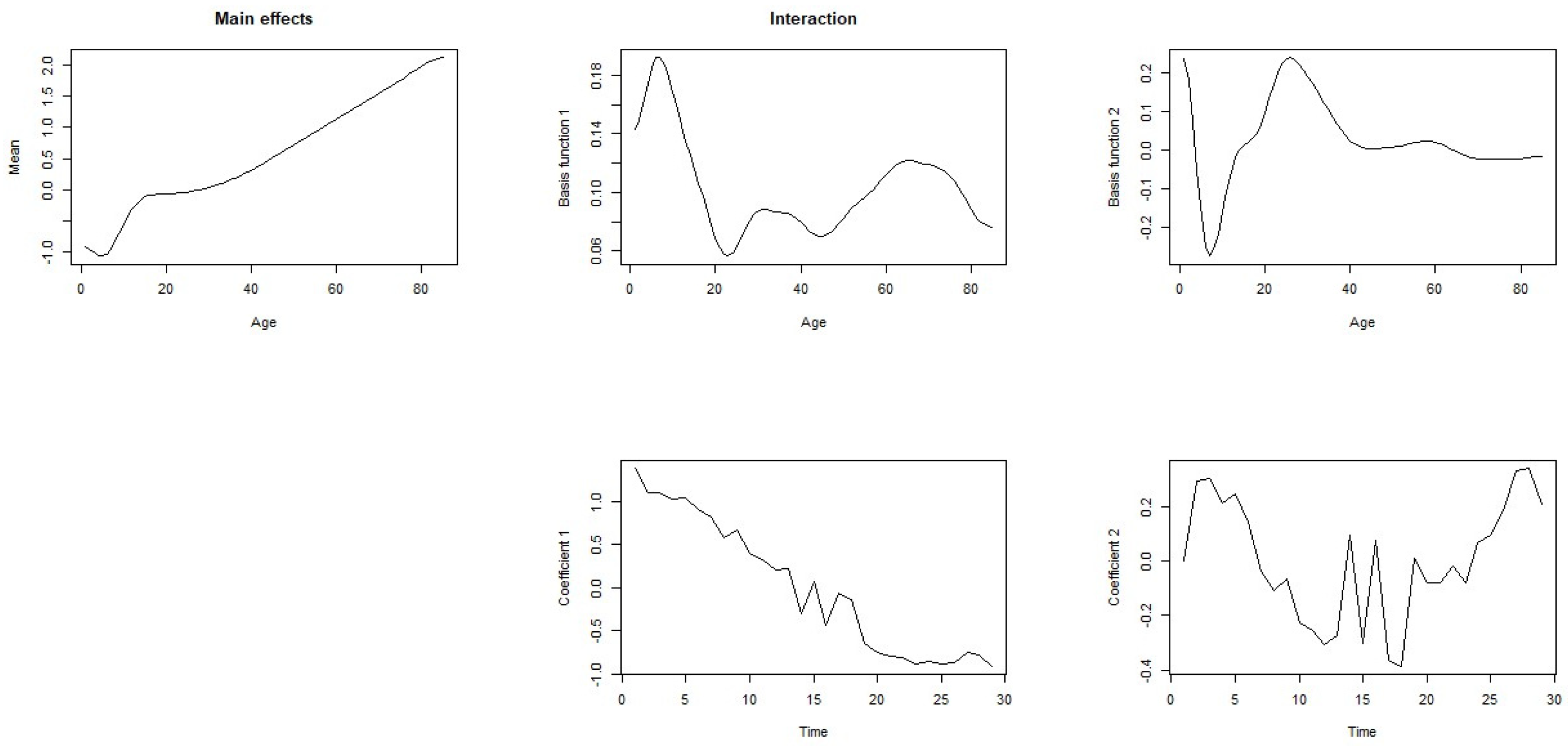
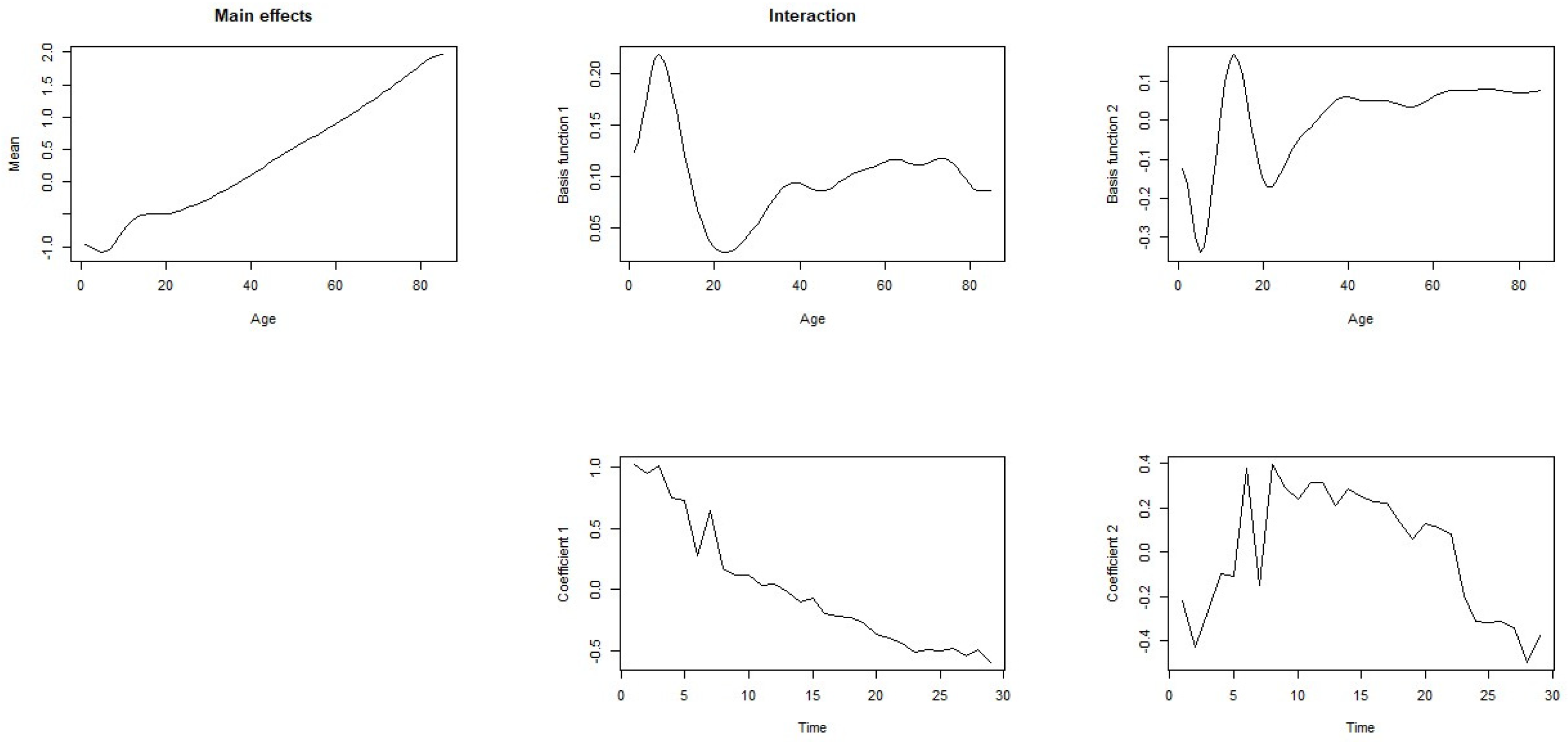
2.3. Functional Principal Component Regression (FPCR)

The theoretical, methodological, and practical aspects of functional principal component analysis (FPCA) have been extensively studied in the functional data analysis literature, since it allows finite dimensional analysis of a problem that is intrinsically infinite-dimensional (Shang and Hyndman [25]). Numerous examples of using FPCA as an estimation tool in regression problem can be found in different fields of applications, such as breast cancer mortality rate modeling and forecasting (Erbas et al. [26], call volume forecasting Shen and Huang [27], Hall and H-NM [28]), climate forecasting (Shang and Hyndman [25]), demographical modeling and forecasting (Shang and Hyndman [25]; Hyndman et al. [21]).

At a population level, under FPCA settings, a smoothed stochastic process denoted by $f\left(x\right)=\left\{f_1\left(x\right),\cdots ,f_n\left(x\right)\right\}$ in Equation (1) can be decomposed into the mean function and the sum of the products of orthogonal functional principal components and uncorrelated principal component scores. It can be expressed as

$$\begin{gathered} f_t\left(x\right)=\mu \left(x\right)+\sum _{k=1}^{\infty }{\beta }_{t, k} {\varnothing }_k\left(x\right) \\ =\mu \left(x\right)+{\sum }_{k=1}^K{\beta }_{t, k} {\varnothing }_k\left(x\right)+e_t(x) \end{gathered}$$

(3)

where, underlying smooth function $f_t\left(x\right)$ belongs to squared integral Hilbert space and $x$ be a set of discrete time points, $\mu \left(x\right)$ is the mean function; $\left\{{\varnothing }_1\left(x\right),\cdots ,{\varnothing }_K\left(x\right)\right\}$ is a set of the first $K$ functional principal components; ${\mathit{\beta }}_1={\left({\beta }_{\mathrm{1,1}}, \cdots ,{\beta }_{1,n}\right)}^{\prime }$ and $\left({\mathit{\beta }}_1,\cdots ,{\mathit{\beta }}_{\mathit{K}}\right)$ denotes a set of principal component scores and ${\mathit{\beta }}_{\mathit{k}}~N\left(0, {\eta }_k\right)$, where ${\eta }_k$ is the $k\mathrm{t}\mathrm{h}$ eigen value of the covariance function

$$c_f\left(r,s\right)=E\left\{\left[f\left(r\right)-\mu \left(r\right)\right]\left[f\left(s\right)-\mu \left(s\right)\right]\right\}$$

(4)

And $e_t\left(x\right)$ is model truncation error function with a mean of zero and a finite variance. Equation (2) provides dimension reduction as the first K terms often serve a good approximation to the infinite terms and thus smoothed function $f\left(x\right)$ is adequately summarized by the K dimensional vector $\left({\mathit{\beta }}_1,\cdots ,{\mathit{\beta }}_{\mathit{K}}\right)$. Here, using the formula defined in Shang and Hyndman [25], the optimal value of K is chosen as the minimum that reaches a certain level of the proportion of total variance explained by the K leading components such that

$$K=\underset{K\ge 1}{\mathrm{argmin}}\left\{{\sum }_{k=1}^K\widehat{{\eta }_k}/{\sum }_{k=1}^{\infty }\widehat{{\eta }_k} {\mathbf{1}}_{\left\{\widehat{{\eta }_k}>0\right\}} \ge \delta \right\}.$$

where $\delta =\mathrm{0,9}$, ${\mathbf{1}}_{\left\{\widehat{{\eta }_k}>0\right\}}$ is used to exclude possible zero eigenvalues with binary indicator function $\mathbf{1}\left\{·\right\}$. In a dense and regularly spaced functional time series, the estimated mean function and the covariance function are shown to be consistent under the weak dependency (Haberman and Kokoxzka [13]). From the empirical covariance function, we can extract empirical functional principal component functions $\mathcal{B}=\left\{\widehat{{\varnothing }_1}\left(x\right),\cdots ,\widehat{{\varnothing }_{K }}\left(x\right)\right\}$ using singular value decomposition. By conditioning on the set of smoothed functions $f\left(x\right)=\left\{f_1\left(x\right),\cdots ,f_n\left(x\right)\right\}$ and the estimated functional principal component $\mathcal{B}$, the h-step ahead forecasts of $y_{n+h}\left(x\right)$ can be obtained as

$${\widehat{y}}_{n+h|n}\left(x\right)=E\left[y_{n+h}\left(x\right)|f\left(x\right),\mathcal{B}\right]=\widehat{\mu }\left(x\right)+{\sum }_{k=1}^K{\widehat{\beta }}_{n+h|n,k}{\widehat{\varnothing }}_k\left(x\right)$$

(5)

where ${\widehat{\beta }}_{n+h|n,k}$ denotes the h-step ahead forecasts of ${\beta }_{n+h|k}$ using a univariate time series forecasting method, which can handle non-stationarity of the principal component scores.

2.4. A Univariate Time Series Forecasting Method

To obtain ${\widehat{\beta }}_{n+h|n,k}$, a univariate time series forecasting method namely autoregressive integrated moving average (ARIMA) method has been considered (Hyndman and Shang [29]). This method is helpful to deal with nonstationary series which contains stochastic trend component. Since the annual age-specific mortality rates for total, male and female series do not contain any seasonality, the ARIMA has a general form of

$$\left(1-{\psi }_{1}B-\cdots , {\psi }_m{B}^m\right){\left(1-B\right)}^d{\mathit{\beta }}_{\mathit{k}}=\alpha +\left(1+{\theta }_{1}B+\cdots +{\psi }_n{B}^n\right){\mathit{w}}_{\mathit{k}}$$

where $\alpha$ represents the intercept, $\left({\psi }_1, \cdots ,{\psi }_m\right)$ are the coefficients associated with autoregressive part, $\left({\theta }_1, \cdots ,{\theta }_n\right)$ are the coefficients associated with moving average part, $B$ denote the backshift operator, d denotes the differencing operator and ${\mathit{w}}_{\mathit{k}}$ represents a white-noise terms. To determine the optimal value of orders for autoregressive, moving average and differencing part, we used automatic algorithm of Hyndman and Khandakar [30]). Once we determine the value of d, the orders of m and n are selected based on the optimal Akaike information criterion (AIC) with a correction for small sample sizes. Once we identified the best ARIMA model, maximum likelihood method can then be used to estimate the parameters of that model.

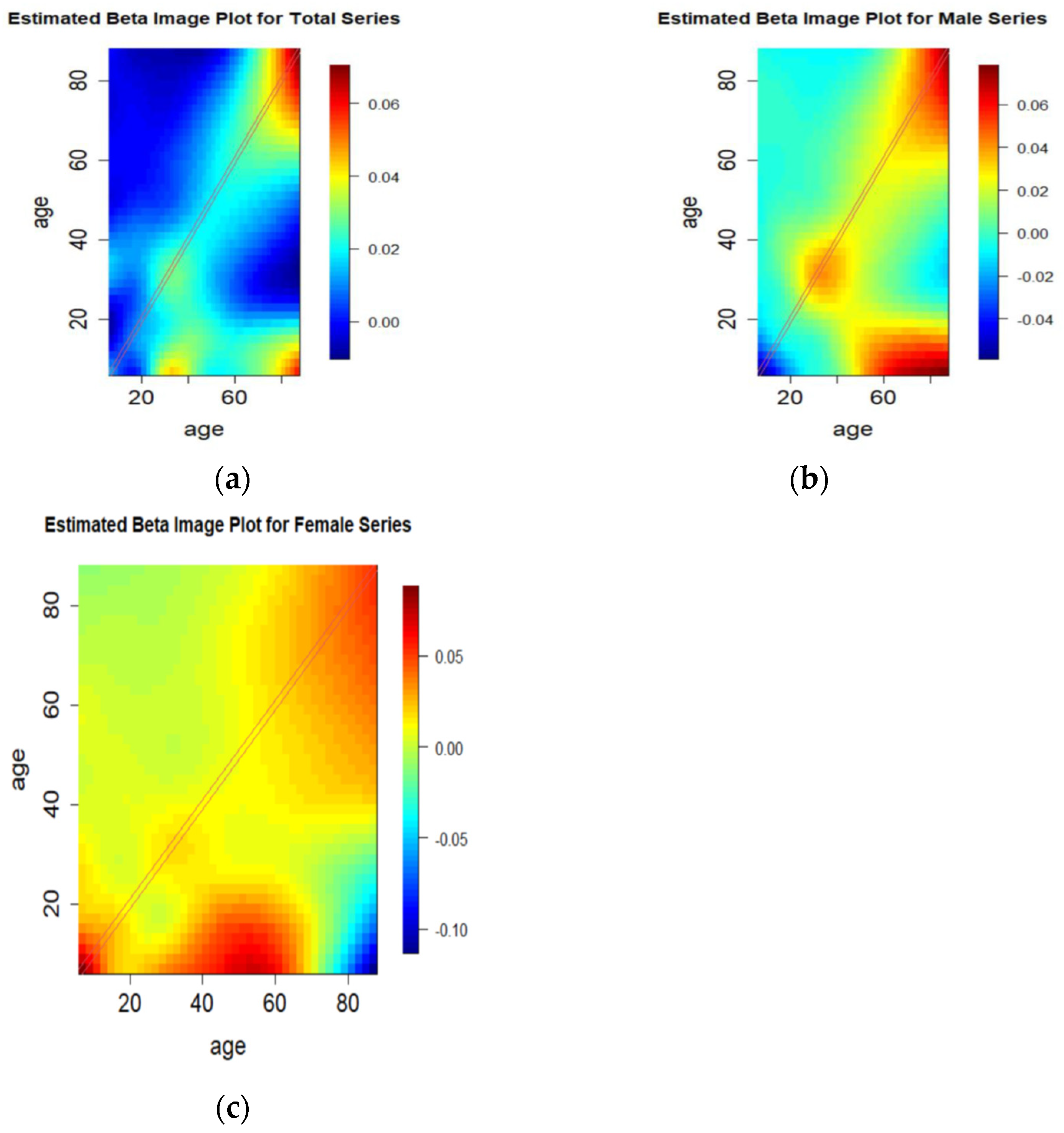
2.5. Functional Autoregressive Process (FAR) of Order One

Bosq [31] introduced the functional autoregressive (fAR) process of order 1, and derived one-step ahead forecasts that are based on a regularized form of the Yule-Walker equations. It is a direct extension of function-on-function linear model under the functional data framework (Ramsay and Silverman [15]). In this model, we would like to use $y_{t-1}\left(x\right)$ to predict $y_t\left(x\right)$ i.e., to measure the impact of one year age differences on mortality series for Canadian population. $y_t\left(x\right)$ is denoted as fAR (1) and defined as

$$y_t\left(x\right)={\beta }_0\left(x\right)+\int \beta \left(z,x\right)y_{t-1}\left(x\right)dx+{\in }_t(x)$$

(6)

Here, $y_t\left(x\right)$ was the observed mortality rate for age $x$ in year $t$; we assume that $y_t\left(x\right)$ depends on $y_{t-1}\left(x\right)$ other than the current time and $\beta \left(z,x\right)$ is the coefficient function defined as $\beta \left(z,x\right)=\sum _{j=1}^J\sum _{k=1}^K{b}_{jk}{\phi }_j\left(z\right){\varnothing }_k\left(x\right)$. Here, we have used two basis functions for two different time points (ages) $z$ and $x$. The two basis functions may be different but for simplicity we used the same basis function for estimating the coefficient function. Details of estimation and inference procedure can be found in Bosq [31]. Here, ${\in }_t\left(x\right)$ is a stochastic process with mean zero and covariance function $\gamma \left(z,x\right)=cov\left\{{\in }_t\left(z\right),{\in }_t\left(x\right)\right\}, \forall t.$

2.6. Prediction Interval and Forecast Accuracy

To construct prediction interval, we calculate the forecast variance that follows from Equations (1) and (3). Because of orthogonality, the forecast variance can be approximated by the sum of component variances.

$${\xi }_{n+h}\left(x\right)=Var\left[y_{n+h}\left(x\right)|f\left(x\right),\mathcal{B}\right]={\sigma }_{\mu }^2\left(x\right)+{\sum }_{k=1}^K{u}_{n+h,k}{\widehat{\varnothing }}_k^2\left(x\right)+\upsilon \left(x\right)+{\sigma }_{n+h}^2\left(x\right)$$

where $u_{n+h,k}=Var\left({\beta }_{n+h,k}|{\beta }_{1,k},\cdots ,{\beta }_{n,k}\right)$ can be obtained from the time series, and the model error variance $\upsilon \left(x\right)$ is estimated by averaging error terms for each $x$, and ${\sigma }_{\mu }^2\left(x\right)$ and ${\sigma }_{n+h}^2\left(x\right)$ can be obtained from the nonparametric smoothing method used. Based on the normality assumption, the $100\left(1-\alpha \right)\%$ prediction interval for $y_{n+h}\left(x\right)$ is constructed as ${\widehat{y}}_{n+h|n}(x)\pm z_{\alpha }\sqrt{{\xi }_{n+h}\left(x\right)}$.

Again, let $e_{n,h}\left(x\right)=y_{n+h}\left(x\right)-$ ${\widehat{y}}_{n+h|n}\left(x\right)$ denote the forecast error for Equation (5). We could then obtain the minimum value of the integrated squared forecast error which is defined as

$${ISFE}_n\left(h\right)=\int e_{n,h}^2\left(x\right)dx$$

We fit the model to data up to time t and predict the next s period to obtain ${ISFE}_n\left(h\right),h=1,\cdots ,s$. We have used a readily available R addon packages “demography” (Hyndman et al. [32]), “forecast” (Hyndman et al. [33]), “rainbow” (Shang and Hyndman [34]), “fda”(Ramsay et al. [35]) and “ftsa”(Hyndman and Shang [36]) to produce figures and analyzing the data respectively.

2.7. Evaluation of Interval Forecast Accuracy

To assess interval forecast accuracy, we use the interval score of Gneiting and Raftery [37]. For each year in the forecasting period, one-year-ahead to 10 years ahead prediction intervals were calculated at the $\left(1-\alpha \right)\times 100\%$ prediction interval, with lower and upper bounds that are predictive quantiles at $\alpha /2$ and $1-\alpha /2$. A scoring rule defined in Geniting and Rafery [37] for the interval forecast at age $x_i$ is as follows:

$$M_{\alpha }\left(x_l,x_u,x_i\right)=\left(x_u-x_l\right)+\frac{2}{\alpha }\left(x_l-x_i\right)I\left(x_i<x_l\right)+\frac{2}{\alpha }\left(x_i-x_u\right)I\left(x_i>x_u\right)$$

where, $I\left\{·\right\}$ represents the binary indicator function, $x_l$ and $x_u$ denote the lower and upper predictive quantiles at $\alpha /2$ and $1-\alpha /2$, and $\alpha$ denotes the level of significance. A forecaster is looking for narrow prediction intervals. For different ages and years in the forecasting period, we consider the mean interval scores as defined in Gneiting and Katzfuss [38].

3. Results

In this study we demonstrate the methodology using demographic data-annual age-specific mortality rates of three different series: total, male and female population in Canada. For this we have $y_t\left(x_i\right)=\log \left(m_t\left(x_i\right)\right)$ where $m_t\left(x_i\right)$ denotes the mortality rate for age $x_i$ in year t.

Figure 1 shows three years of total death rates in Canada. The dynamic behavior of the underlying curve is relatively complicated and is clear from Figure 1. For example, the ‘bump’ around 18–19 years of age higher relative to nearby ages in 1991 than in the other years plotted. Furthermore, the general drop in mortality over time is not uniform over ages or time as observed in nearby ages before 20, for three time periods over ten years apart. First, we transformed our three different mortality series: total, male and female into functional objects. We represented our discrete data with B-spline basis functions since our data shows monotonicity. Next, we obtained the best estimated smoothed curves $f\left(t\right)$ by eliminating the contribution of the errors and noise presented in the functional objects. To do that we used a penalized regression spline, constrained to be monotonic. We weight the penalized regression splines using the inverse of variance ${\sigma }_t^2\left(x_i\right)$. The order-selection procedure described in functional principal component regression section led to a model with $K=2$ basis functions. The robustness parameter was set via cross validation.

Figure 2 shows rainbow plots of the total, male and female age-specific smoothed log mortality rates in Canada from 1991 to 2019. The time ordering of the curves follows the color order of a rainbow, where curves from the distant past are shown in red and the more recent curves are shown in purple. The changing shape of the curves over time and relatively complex dynamic nature around early ages are clear from the figure as well. Further analyses such as descriptive and forecasting are based on these functional data.

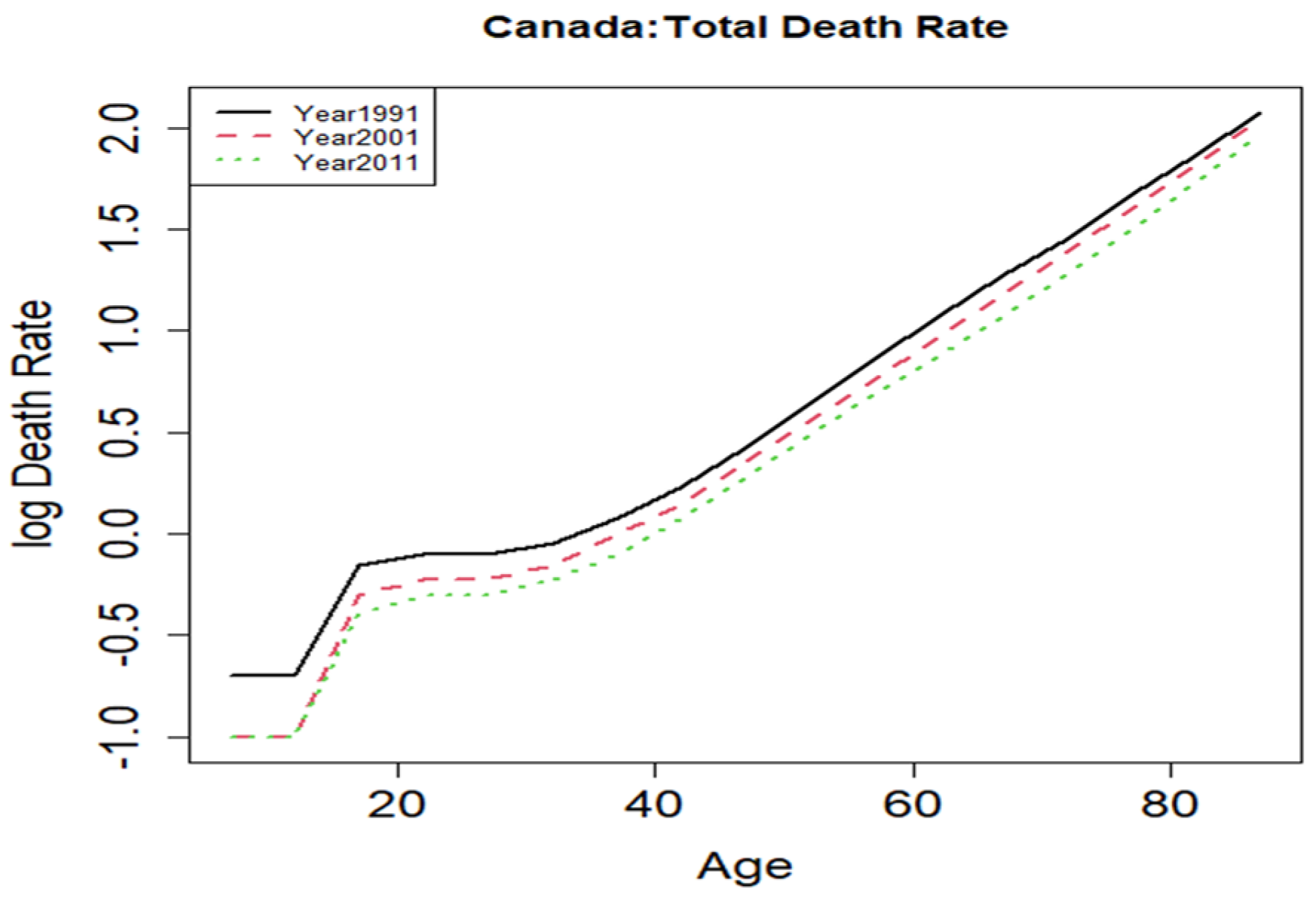
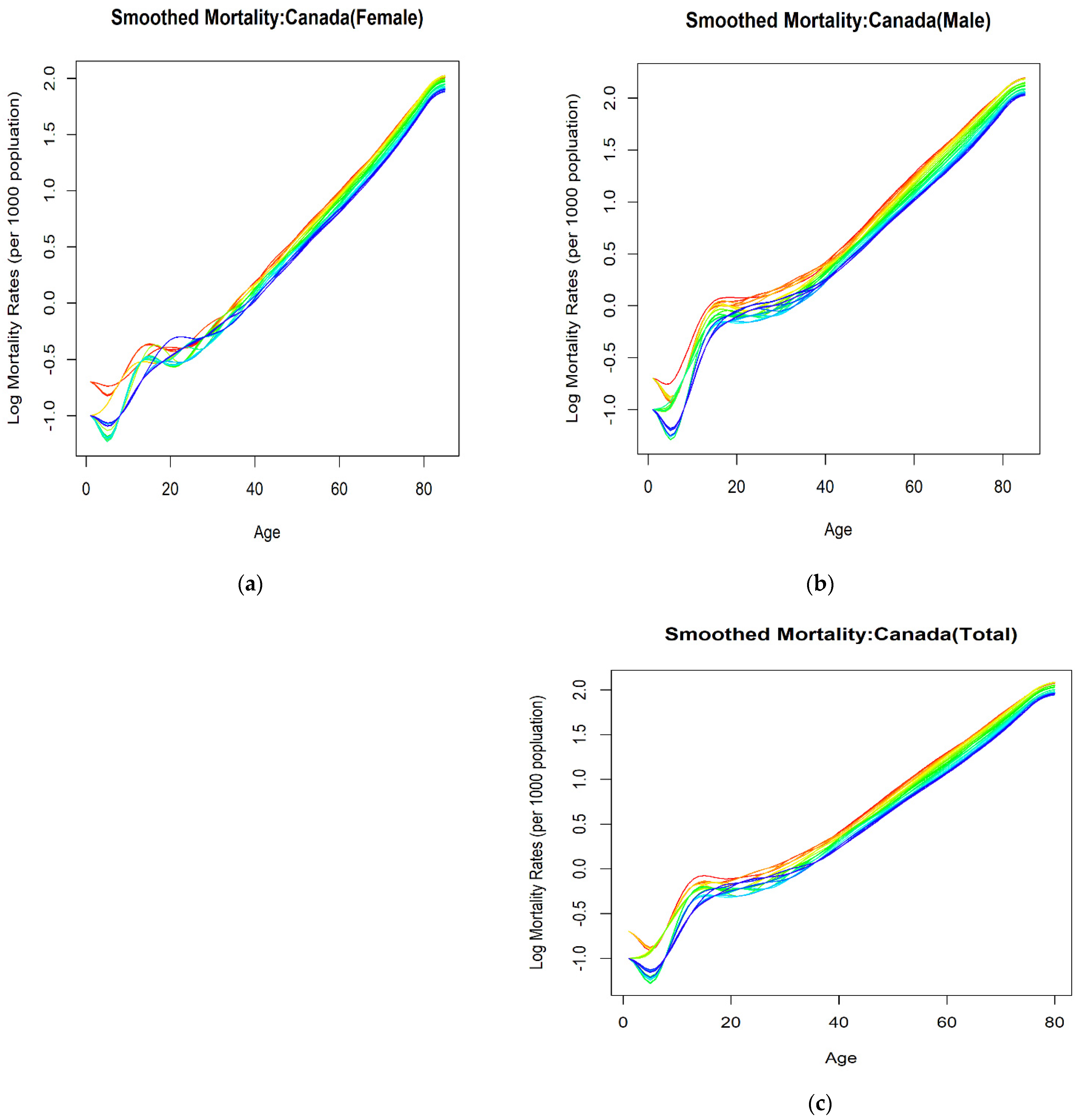
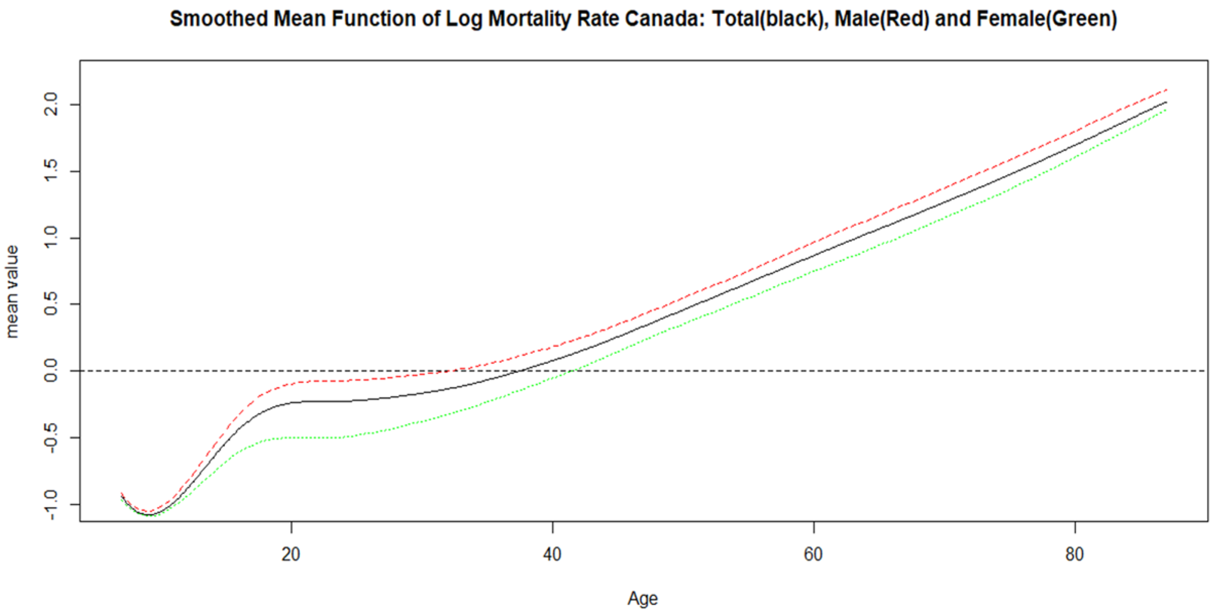
3.1. Temporal Patterns of Mortality Rates

Figure 3 displays the mean functions of the functional data for three different series. From Figure 3, it is apparent that the general increase of mean function in mortality over time is observed for male group of population compared to total and female population just after age of 20. Furthermore, the ‘bumps’ was around the age of 20 for male group, however it was around the age of 15–17 years for female group and around 18–19 years for total population respectively. The high variation was also found nearby 15–20 years of ages compared to other discreate points for each series.

3.2. Age-Specific Mortality Forecasting for Canada

Figure 4 shows the forecasts of Canadian mortality rate data for: total, male and female groups from 2020 to 2029 (ten years) highlighted in rainbow color. The time ordering of the curves follows the color order of a rainbow, where curves from the distant past are shown in red and the more recent curves are shown in purple. Compared to total and female group, highest bumps occur around age 20 years for male group. However, a complex dynamic behavior for next ten years was found around early ages for female groups with relatively a similar pattern at nearby 20 years of ages. Besides these, after middle years of age (around 40 years), forecasted mortality rates for next ten years for all series show general increase over the time and ages.

Forecasts of mortality rates in 2020 for each series are shown in Figure 5 along with 95% prediction interval computed using the variance given in prediction interval and forecast accuracy section. Clearly the greatest forecast variation observed around early and middle years of ages for all the series. In addition, we obtained forecasts of mortality rates in 2020 for each series based on the traditional univariate time series forecasting method such as exponential smoothing (ets) and obtained mean interval forecast score. We observed that for forecasting age-specific mortality, functional time series method produces more narrower interval forecasts than traditional univariate time series forecasting method (See Supplementary File: Figure S1 and Table S1).

The fitted principal components (PCs) (which corresponds to basis functions 1 and 2) and associated scores (corresponds to basis coefficients) are shown in Figure 6 for total mortality series in Canada. From Figure 6, it is evident that basis function 1 (first PC) primarily models mortality changes in children, and second basis function (2nd PC) models the difference between young adults and those over 40. Furthermore, it is clear from principal component scores that child mortality rates have decreased throughout the whole data period, while the difference between mortality rates for young people and those over 40 has only been decreasing since roughly 2003 and has levelled off in the last ten years of data.

Figure 7 and Figure 8 display the basis functions (principal components) and associated coefficients (scores) for the Canadian male and female mortality series. A decomposition of $K=2$ has been used. From Figure 7, it is evident that basis function 1 (PCA 1) primarily models mortality changes in children, and second basis function (PCA2) models the difference between youth and those over 30. While the difference between youth and those over 30 has only started decreasing since approximately 2008 and has levelled off in the last decade of the data, the death rates for children have decreased over the whole data period. Similarly, from Figure 8, it is evident that basis function 1 (PCA 1) primarily models mortality changes in children, and second basis function (PCA2) models the difference between young adults and those over 25. The disparity between young people and those over 25 has only been decreasing since approximately 1997 and has plateaued in the last decade of data, but the mortality rates for children have decreased during the whole data period.

3.3. Age Difference in Forecasted Mortality Rate Using FAR(1)

Functional autoregressive model of order one is used to determine the impact age differences in mortality series. Figure 9 is used to display coefficients to assess the impact of one year age differences in total, male and female mortality series for Canadian population. In Figure 9, for total series, (a) the red lines indicate the moderate effect of total mortality rate of current year on the next year when the age is one year apart. On the other hand, for male series (b) the red line indicates the strong effect of male mortality rate of current year on the next year when the age is one year apart (around middle age group). Similarly, for female series (c) the red line indicates the strong effect of female mortality rate of current year on the next year when the age is one year apart (around the whole entire age intervals).

4. Discussion

This paper introduces an applied approach of forecasting demographic series: age-specific mortality series-using functional time series analysis technique and compare the predicted continuous distribution rather than observed discrete values. Applied approach is suitable for any situation where multiple time series are observed and where the observations in each period can be considered as arising from an underlying smooth curve. In general, Hyndman and Ullah [9] discussed that this approach performs better forecasting results compared to Lee and Carter [10] approach to mortality forecasting. We have demonstrated this method on Canadian annual age-specific mortality rates for total, male and female groups separately.

For each series, we have considered the penalized regression splines (Wood [24]) basis function for transforming discrete data to the smoothed functional series. The plot of smoothing curves for average functions for each series can be used to identify increase or decrease mortality pattern over time across different age groups for Canadian population. We have also shown how to use functional principal component regression and functional autoregressive model to forecast and examine effects of age differences in mortality series respectively.

Our results reveal that it is apparent that the general increase of mean function in mortality over time is observed for male group of population compared to total and female population just after the age of 20. Furthermore, the ‘bumps’ was around the age of 20 for male group, however it was around the age of 15–17 years for female group and around 18–19 years for total population respectively. The high variation was also found nearby 15–20 years of ages compared to other discreate points for each series. This temporal pattern of change in mean function could not be uncovered by analysis on the observed discrete data.

We have also presented a way of constructing uniform and pointwise prediction interval for each of the series for next ten years. For this forecasted period, it is evident that compared to total and female group, highest bumps occur around age 20 years for male group. However, a complex dynamic behavior for next ten years was found around early ages for female groups along with relatively a similar pattern at nearby 20 years of ages. Besides these, after middle years of age (around 40 years), forecasted mortality rates for next ten years for all series shows general increase over the time and ages.

The result of functional principal component regression reveals complex dynamic patterns of mortality series over time and ages. For total series, it indicates that that the mortality rates for children have dropped over the whole data period, while the difference between young adults and those over 40 has only been falling since about 2003 and has leveled off in the last decade of the data. Furthermore, for male and female groups it is evident that the mortality rates for children have dropped over the whole data period, while the difference between youth and those over 40 has only been falling since about 2008 and has leveled off in the last decade of the data, and the difference between young adults and those over 40 has only been falling since about 1997 and has leveled off in the last decade of the data, respectively.

Our results confirm moderate to strong impact of age differences on Canadian age-specific mortality series. For total series, we found moderate effect of total mortality rate of current year on the next year when the age is one year apart. On the other hand, for male and female groups we observed the strong effect of male mortality rate of current year on the next year when the age is one year apart around middle age group and for the entire age intervals respectively.

This research looks at how an underlying forecasting technique can be used to estimate one of the demographic components of a national population projection. No study is beyond limitations. Our study also faced one limitation such as to find the uncertainty of estimates for smooth functions in Figure 2, (to make an statement such as weather increase in mortality observed in males compared to total and females are statistically significant), it was not possible to obtain 95% PIs for those curves in our study. For future research, it could be interesting to take into account some additional available information regarding sub-national level (e.g., geography), cause-of-death, socio-economic status and cohort effects in forecasting the disaggregated mortality series. The functional time series analysis technique could be adapted for where multiple time series are observed and where the observations in each period can be considered as arising from an underlying smooth curve.

Understanding the temporal trends of age-specific mortality series is critical in demography and the formulation of age-related policies. It is critical that such pattern discovery is based on the best available statistical modeling approaches to minimize possible prediction errors. The functional time series analysis can reveal the temporal variability, rate of change, and specific age-group modelling for mortality series, as well as the effect of age differences, providing additional insight for forecasting age-related policies, future population age structure, and hospital resource management (Kuschel et al. [39]). Wider use of functional time series analysis (FTSA) to obtain more accurate estimates in public health, demography, and insurance policy studies should be considered.

References

1. Canadian Human Mortality Database 2014. Universite de Montreal (Canada), University of Californica Berkley (USA), and Max Planck Institute for Demographic Research (Germany). Available online: http://www.bdlc.umontreal.ca (accessed on 2 June 2022).
2. Statistics Canada. Data Table 13-10-0710-01. Available online: https://www150.statcan.gc.ca/t1/tbl1/en/tv.action?pid=1310071001 (accessed on 29 August 2022).
3. Bourheau, R.; Ouellette, N. Trends, patterns, and differentials in Canadian mortality over nearly a century (1921–2011). Canaidan Stud. Popul. 2016, 43, 48–77. [Google Scholar] [CrossRef]
4. Bah, S.M.; Rajulton, F. Has Canadian mortality entered the fourth stage of the epidemiologic transition. Can. Stud. Popul. 1991, 18, 18–41. [Google Scholar] [CrossRef]
5. Bourbearu, R. Canadian mortality in perspective: A comparison with the United States and other developed courntries. Can. Stud. Popul. 2002, 29, 313–369. [Google Scholar] [CrossRef]
6. Lussier, M.-H.; Bourbeaue, R.; Choiniere, R. Does the recent evolution of Candian mortality agree with the epidemiological transition theory? Demogr. Res. 2008, 18, 531–568. [Google Scholar] [CrossRef]
7. Mandich, S.; Margolis, R. Changes in disability-free life expectancy in Canada between 1994 and 2007. Can. Stud. Popul. 2014, 41, 192–208. [Google Scholar]
8. Jasilionis, D. Reversals in life expectancy in high income countries? BMJ 2018, 362, k3399. [Google Scholar] [CrossRef]
9. Hyndman, R.J.; Ullah, S. Robust forecasting of mortality and fertility rates: A Functional data approach. Comput. Stat. Data Anal. 2007, 51, 4942–4956. [Google Scholar] [CrossRef]
10. Lee, R.D.; Carter, L.R. Modeling and forecasting U.S. mortality. J. Am. Stat. Assoc. 1992, 87, 659–671. [Google Scholar] [CrossRef]
11. Lee, R.D.; Miller, T. Evaluating the performance of Lee-Carter method for forecasting mortality. Demography 2001, 38, 537–549. [Google Scholar] [CrossRef]
12. Booth, H.; Maindonald, J.; Smith, L. Applying Lee-Carter under conditions of variable mortality decline. Popul. Stud. 2002, 56, 325–336. [Google Scholar] [CrossRef]
13. Renshaw, A.E.; Haberman, S. Lee-Carter mortality forecasting: A parallel generalized linear modeling appraoch for England and Wales mortality projections. Appl. Stat. 2003, 52, 119–137. [Google Scholar] [CrossRef]
14. De Jong, P.; Tickle, L. Extending Lee-Carter mortality forecasting. Math. Popul. Stud. 2006, 13, 1–18. [Google Scholar] [CrossRef]
15. Ramsay, J.O.; Silverman, B.W. Functional Data Analysis; Springer: New York, NY, USA, 2005. [Google Scholar]
16. Aguilera, A.M.; Escabias, M.; Valdarrama, M.J. Using principal components for estimating logistic regression with high dimensitional multicolinear data. Comput. Stat. Data Anal. 2006, 50, 1905–1924. [Google Scholar] [CrossRef]
17. Shang, H.L.; Hyndman, R.J. Grouped Functional Time Series Forecasting: An Application to Age-Specific Mortality Rates. J. Comput. Graph. Stat. 2017, 26, 330–343. [Google Scholar] [CrossRef]
18. Wang, J.-L.; Chiou, J.-M.; Müller, H.-G. Functional Data Analysis. Annu. Rev. Stat. Its Appl. 2016, 3, 257–295. [Google Scholar] [CrossRef]
19. Thakallapelli, A.; Ghosh, S.; Kamalasadan, S. Real-time Frequency Based Reduced Order Modeling of Large Power Grid. In Proceedings of the Power and Energy Society General Meeting, Boston, MA, USA, 17–21 July 2016. [Google Scholar]
20. Pitor, K.; Matthew, R. Introduction to Functional Data Analysis, 1st ed.; CRC Press: Boca Raton, FL, USA; Taylor and Francis Group: New York, NY, USA, 2017. [Google Scholar]
21. Hyndman, R.J.; Zeng, Y.; Shang, H.L. Forecasting the old-age dependency ratio to determine a sustainable pension age. Aust. N. Z. J. Stat. 2021, 63, 241–256. [Google Scholar] [CrossRef]
22. Organization for Economic Co-Operation and Development (OECD). OECD Health Statistics 2014. Website: Public Expenditure on Health, % Total Expenditure on Health. Available online: http://stats.orecd.org/Index.aspx?DataSetCode=SHA (accessed on 1 August 2022).
23. Hörmann, S.; Kokoszka, P. Weakly dependent functional data. Ann. Stat. 2010, 38, 1845–1884. [Google Scholar] [CrossRef]
24. Wood, S.N. Stable and Efficient Multiple Smoothing Parameter Estimation for Generalized Additive Models. J. Am. Stat. Assoc. 2004, 99, 673–686. [Google Scholar] [CrossRef]
25. Shang, H.L.; RobJ, H. Nonparametric time series forecasting with dynamic updating. Math. Comput. Simul. 2011, 81, 1310–1324. [Google Scholar] [CrossRef]
26. Erbas, B.; Akram, M.; Gertig, D.M.; English, D.; Hopper, J.L.; Kavanagh, A.M.; Hyndman, R. Using Functional Data Analysis Models to Estimate Future Time Trends in Age-Specific Breast Cancer Mortality for the United States and England–Wales. J. Epidemiol. 2010, 20, 159–165. [Google Scholar] [CrossRef]
27. Shen, H.; Huang, J.Z. Interday Forecasting and Intraday Updating of Call Center Arrivals. Manuf. Serv. Oper. Manag. 2008, 10, 391–410. [Google Scholar] [CrossRef]
28. Hall, P.; Hosseini-Nasab, M. On properties of functional principal components analysis. J. R Stat. Soc. B 2006, 65, 109–126. [Google Scholar] [CrossRef]
29. Hyndman, R.J.; Shang, H.L. Forecasting functional time series. J. Korean Stat. Soc. 2009, 38, 199–211. [Google Scholar] [CrossRef]
30. Hyndman, R.J.; Khandakar, Y. Automatic Time Series Forecasting: The forecast Package for R. J. Stat. Softw. 2008, 27, 1–22. [Google Scholar] [CrossRef]
31. Bosq, D. Implementation of Functional Autoregressive Predictors and Numerical Applications. In Linear Process Functioal Spaces; Springer: New York, NY, USA, 2000; pp. 237–266. [Google Scholar]
32. Hyndman, R.; Booth, H.; Tickle, L.; Maindonald, J.; Wood, S.; R Core Team. Demography: Forecasting Mortality, Migration and Population Data. 2023. R Package Version 2.0. Available online: https://github.com/robjhyndman/demography (accessed on 1 August 2022).
33. Hyndman, R.; Athanasopoulos, G.; Bergmeir, C.; Caceres, G.; Chhay, L.; Kuroptev, K.; Wild, M.O. Forecast: Forecasting Functions for Time Series and Linear Models. 2023. R Package Version 8.21. Available online: https://pkg.robjhyndman.com/forecast/ (accessed on 1 August 2022).
34. Shang, H.L.; Hyndman, R. Rainbow: Bagplots, Boxplots and Rainbow Plots for Functional Data. 2022. R Package Version 3.7. Available online: https://orcid.org/000-0003-1769-6430 (accessed on 1 August 2022).
35. Ramsay, J.; Hooker, G.; Graves, S. fda: Functional Data Analysis. 2023. R Package Version 6.1.4. Available online: http://www.functionaldata.org (accessed on 1 August 2022).
36. Hyndman, J.; Shang, H.L. ftsa: Funtional Time Series Analysis. 2013. R Package Version 3.8. Available online: http://CRAN.R-project.org/package=ftsa (accessed on 1 August 2022).
37. Gneiting, T.; Raftery, A.E. Strictly proper scoring rules, prediction and estimation. J. Am. Stat. Assoc. 2007, 102, 359–378. [Google Scholar] [CrossRef]
38. Gneiting, T.; Katzfuss, M. Probabilistic forecasting. Annu. Rev. Stat. Appl. 2014, 1, 125–151. [Google Scholar] [CrossRef]
39. Kuschel, K.; Carrasco, R.; Idrovo-Aguirre, B.J.; Duran, C.; Contreras-Reyes, J.E. Preparing Cities for Future Pandemics: Unraveling the Influence of Urban and Housing Variables on COVID-19 Incidence in Santiago de Chile. Healthcare 2023, 11, 2259. [Google Scholar] [CrossRef]
Figure 1. Plot of the total mortality rates in Canada.
Mathematics 11 03808 g001
Figure 2. Plot of smoothed functional mortality series: (a) Female mortality series; (b) male series and (c) total series (both sexes). Curves from the distant past are shown in red and the more recent curves are shown in purple.
Mathematics 11 03808 g002
Figure 3. Mean functions for smoothed functional mortality series: total mortality series (black); male mortality series(red) and female mortality series (green).
Mathematics 11 03808 g003
Figure 4. Ten year forecasted mortality rate of Canada for both sexes (left), male (middle) and female (right). Red color represents year 2020 and blue color represents year 2029.
Mathematics 11 03808 g004
Figure 5. Interval (95% Prediction Interval) and point forecasted value of 2020 MR Canada: total (both sexes), male and female series. Red lines represent lower and upper values of 95% PI and black lines represents point forecasted values.
Mathematics 11 03808 g005
Figure 6. Principal component regression output for Canada: total mortality series.
Mathematics 11 03808 g006
Figure 7. Principal component regression output for Canada: male mortality series.
Mathematics 11 03808 g007
Figure 8. Principal component regression output for Canada: female mortality series.
Mathematics 11 03808 g008
Figure 9. Image plot of estimated betas for (a) total, (b) male and (c) female mortality series using FAR (1) model. The lines represent high correlation.
Mathematics 11 03808 g009
Disclaimer/Publisher’s Note: The statements, opinions and data contained in all publications are solely those of the individual author(s) and contributor(s) and not of MDPI and/or the editor(s). MDPI and/or the editor(s) disclaim responsibility for any injury to people or property resulting from any ideas, methods, instructions or products referred to in the content.