An Efficient Hybrid Multi-Objective Optimization Method Coupling Global Evolutionary and Local Gradient Searches for Solving Aerodynamic Optimization Problems

Abstract

Aerodynamic shape optimization is frequently complicated and challenging due to the involvement of multiple objectives, large-scale decision variables, and expensive cost function evaluation. This paper presents a bilayer parallel hybrid algorithm framework coupling multi-objective local search and global evolution mechanism to improve the optimization efficiency and convergence accuracy in high-dimensional design space. Specifically, an efficient multi-objective hybrid algorithm (MOHA) and a gradient-based surrogate-assisted multi-objective hybrid algorithm (GS-MOHA) are developed under this framework. In MOHA, a novel multi-objective gradient operator is proposed to accelerate the exploration of the Pareto front, and it introduces new individuals to enhance the diversity of the population. Afterward, MOHA achieves a trade-off between exploitation and exploration by selecting elite individuals in the local search space during the evolutionary process. Furthermore, a surrogate-assisted hybrid algorithm based on the gradient-enhanced Kriging with the partial least squares(GEKPLS) approach is established to improve the engineering applicability of MOHA. The optimization results of benchmark functions demonstrate that MOHA is less constrained by dimensionality and can solve multi-objective optimization problems (MOPs) with up to 1000 decision variables. Compared to existing MOEAs, MOHA demonstrates notable enhancements in optimization efficiency and convergence accuracy, specifically achieving a remarkable 5–10 times increase in efficiency. In addition, the optimization efficiency of GS-MOHA is approximately five times that of MOEA/D-EGO and twice that of K-RVEA in the 30-dimensional test functions. Finally, the multi-objective optimization results of the airfoil shape design validate the effectiveness of the proposed algorithms and their potential for engineering applications.

1. Introduction

Multi-objective optimization techniques are widely used in the field of engineering optimization to reduce the budget of design, particularly in aerodynamic shape design [1,2,3]. However, complex aerodynamic shape design is often faced with large-scale design variables and expensive fitness evaluations. As a result, the efficiency of existing multi-objective algorithms is correspondingly reduced. Their huge computational cost limits the engineering practicality of multi-objective optimization algorithms. Therefore, the development of efficient multi-objective optimization algorithms to reduce computation cost is highly attractive for aerodynamic shape design in engineering optimization.

The common optimization methods mainly include gradient-based algorithms (GBAs) and metaheuristic optimization algorithms [4]. The GBAs start from an initial point and determine the best local search direction by the gradients of the objective and constraint functions with respect to the design variables. Subsequently, the optimal descent step is evaluated and the local search procedure is iterated until the local optimal solution in the vicinity of the initial point is reached. Generally, the weighted sum method is used to convert multiple cost functions into a single integrated cost function to solve multi-objective optimization problems (MOPs).

The two main advantages of GBAs are fast convergence and high accuracy. However, GBAs are also sensitive to starting points and weight vectors and tend to fall into local optimal solutions. Currently, the commonly used gradient-based optimization methods include the quasi-Newton algorithm [5,6], conjugate gradient method [7], and sequential quadratic programming algorithm [8]. As the number of design variables increases, the computational cost of evaluating gradients by using finite difference or complex step methods is prohibitive. Fortunately, the adjoint method proposed by Jameson [9] can be used to calculate the gradient accurately and efficiently. The computational cost of the adjoint method is independent of the dimension of design variables, so it is widely used in the aerodynamic optimization of large-scale decision variables.

Evolutionary algorithms (EAs) are typical metaheuristic algorithms that simulate the biological evolution phenomenon in nature to achieve a search for the global optimal solution [10]. Compared with GBAs, EAs are global methods with high robustness and universality, which can effectively handle complex optimization problems that GBAs find difficult to solve. Although EAs have good global search capabilities, they suffer from problems such as slow convergence and low search efficiency. As a consequence, the adjoint method is almost the only choice in aerodynamic shape design optimization with large-scale decision variables. For example, GBAs are successfully applied to the optimization of wing shape design (with 721 design variables) and blended wing body shape design (with 273 design variables) [11,12].

Most recently, the aerodynamic shape optimization method is developing towards solving MOPs with many objectives; large-scale design variables; the coupling of objective characteristics; and expensive objective calculations. The accuracy and efficiency of the optimization results are directly influenced by the search capability of optimization algorithms. Therefore, multi-objective aerodynamic shape optimization methods face the following several challenges:

(1)

As the number of design variables and objectives increases, the multi-objective evolutionary algorithm (MOEA) requires a larger population size and more iterations to approach the optimal Pareto front (PF), resulting in a significant decrease in optimization efficiency and accuracy.

(2)

Although the existing gradient-based multi-objective optimization algorithms are efficient, they can only obtain local optimal solutions and cannot solve MOPs with arbitrary PF.

(3)

High-fidelity aerodynamic shape optimization is usually calculated using a computational fluid dynamics (CFD) solver based on the Reynolds-Averaged Navier–Stokes (RANS) equations, which makes the aerodynamic analysis very computationally costly.

To address the first two challenges, this paper proposes improved GBAs that can solve MOPs with any type of PF and any number of objective functions. It should be noted that a stochastic weight function is introduced in the weighted sum method and a set of stochastic weights is re-assigned to each individual at each iteration to distinguish it from traditional weighting algorithms. The PF is generated by constantly changing the weights to explore the objective space. Moreover, to avoid the multi-objective gradient-based algorithm (MOGBA) from falling into local optimal solutions, a new multi-objective hybrid algorithm (MOHA) is considered to be developed by combining the evolutionary mechanism in MOEA and the local search mechanism based on the GBA. The core idea of the hybrid algorithm is to design a reasonable hybrid strategy to overcome the shortcomings of each algorithm, thus improving efficiency and accuracy. Through this process, the hybrid algorithms can learn from each other and achieve better overall performance. In several recent studies, researchers have proposed various hybrid strategies to balance diversity and convergence for solving single-objective optimization problems or MOPs [13,14,15]. To improve the optimization efficiency while taking into account the global search capability, a bilayer parallel hybrid strategy is designed in this paper. This hybrid strategy introduces a multi-objective local search mechanism into MOEA using a non-cooperative co-evolutionary approach to improve performance by balancing the global search and local search capabilities of the algorithm.

However, with the development of aerodynamic analysis methods, high-fidelity CFD calculation methods based on solving the RANS equations are gradually eliminating low-fidelity methods such as solving the velocity potential and Euler equations. Meanwhile, the shape parameterization and grid generation of aircraft are becoming increasingly refined. These factors make it possible for a single CFD simulation to take several minutes to several hours. MOEA is the primary source of computational cost, serving as the main driving engine of hybrid algorithms. While MOHA can improve optimization efficiency by reducing the number of algorithm iterations, it cannot reduce the time required for fitness evaluation. The application of MOHA in high-fidelity aerodynamic shape optimization design is hindered as the computational cost remains difficult to accept.

Based on the above descriptions, to overcome problem 3, a popular approach is to use the surrogate model to approximate the objective function. Once the surrogate model is established, the subsequent optimization design can be carried out based on the surrogate model. In engineering optimization, the multi-objective evolutionary algorithm (MOEA) necessitates repetitive and cost-intensive calculations. Conversely, the surrogate-assisted evolutionary algorithm (SAEA) employs surrogate models as substitutes for these costly evaluations. By minimizing the count of expensive fitness evaluations, SAEA effectively achieves the objective of reducing optimization time [16,17,18,19]. In summary, this paper proposes a novel gradient-based surrogate-assisted multi-objective hybrid algorithm (GS-MOHA) by combining a hybrid multi-objective evolutionary algorithm with a metamodel technique. The algorithm enhances the engineering application capability of MOHA in high-dimensional multi-objective optimization for aerodynamic shape design.

The commonly used surrogate models mainly include the polynomial response surface model [20] (RSM), Kriging [21], artificial neural network [22] (ANN), radial basis function network model [23] (RBF) and support vector machine [24] (SVM). However, there is a lack of theoretical guidance in choosing a surrogate model. The Kriging model is a popular choice, which not only has a good approximation ability for nonlinear functions but also provides uncertainty assessment. Many well-known surrogate-assisted multi-objective evolution algorithms use the Kriging model as the approximate model, such as ParEGO [25], MOEA/D-EGO [26], and K-RVEA [27]. After establishing the initial surrogate model, the dynamic surrogate-based optimization algorithm needs to update the surrogate model to improve accuracy, which is achieved by selecting new sample points according to the optimization infill criterion.

Although many algorithms using surrogate models in MOEA have been proposed, there are still many challenges. One is the selection of surrogate models as there is no clear criterion for selecting a suitable type of surrogate model to replace the expensive fitness evaluation. The second is the time cost of training the surrogate model; the training time increases exponentially as the dimension of the design variable increases, sometimes even exceeding the cost of direct CFD simulation. The third aspect involves managing the surrogate model, including determining the optimal timing for updating the model and selecting suitable sample points for the update process. Most SAEAs solve problems with fewer than 10 dimensions of decision variables [17,18,28]. This is mainly because they require more samples and iterations to train the hyperparameters in the model when the dimension increases. To address this issue, we use the gradient-enhanced Kriging with partial least squares (GEKPLS) method to approximate each objective function, and the Kriging model is established by using the objective function values and their gradient information [29]. This gradient-enhanced Kriging (GEK) method improves modeling efficiency in high-dimensional spaces significantly by reducing the number of hyperparameters through dimensionality-reduction techniques.

The remainder of this paper is organized as follows. In Section 2, we briefly recall the difficulties of multi-objective optimization and of the GEKPLS model, as well as the motivation for this paper. Meanwhile, a gradient-based multi-objective algorithm is proposed, which is an improvement on the traditional gradient algorithm. Section 3 and Section 4 present details of the proposed MOHA and GS-MOHA. Section 5 presents an experimental study to validate the excellent performance of the proposed algorithms. In Section 6, the efficiency and engineering applicability of MOHA and GS-MOHA are compared and verified through a multi-objective shape optimization of an airfoil. Finally, the conclusions and future work are drawn in Section 7.

2. Related Work and Motivation

This section first introduces the difficulties of existing multi-objective optimization algorithms when facing high-dimensional optimization. MOGBA is then proposed and validated against MOEA. In addition, the performance of the GEKPLS model is discussed in comparison with ordinary Kriging and GEK models. Finally, the motivation for developing efficient hybrid algorithms in this paper is emphasized.

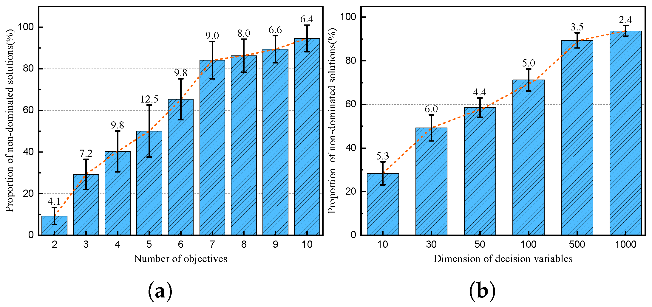
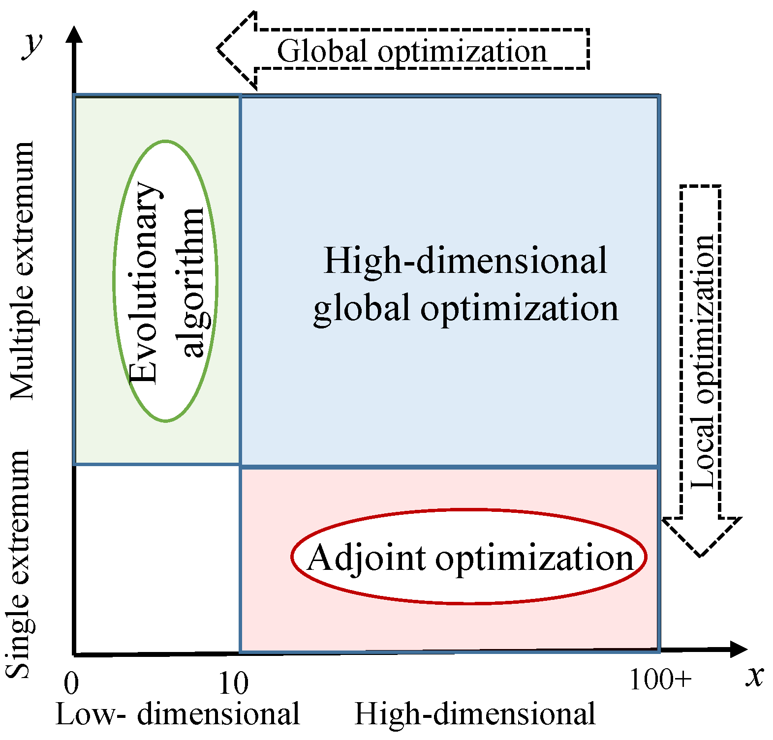
2.1. Difficulties of Multi-Objective Optimization Problems

The MOP involving M objectives can be formulated as follows:

$$\begin{array}{cc}min\hfill & f\left(x\right)={\left(f_1\left(x\right),f_2\left(x\right),\dots ,f_M\left(x\right)\right)}^T\hfill \\ \mathrm{s}.\mathrm{t}.\hfill & g_i\left(x\right)\le 0,i=1,\dots ,p\hfill \\ \hfill & h_j\left(x\right)=0,j=1,\dots ,q\hfill \end{array}$$

(1)

where $x={(x_1,x_2,\cdots ,x_D)}^T\in \Omega$ is the decision vector, and $f={(f_1,f_2,\cdots ,f_M)}^T\in \Lambda$ is the objective vector. All of the decision vectors constitute a known D-dimensional decision space $\Omega$, and all of the objective vectors constitute an unknown M-dimensional objective space $\Lambda$. $g_i\left(x\right)$ is the i inequality constraint, p is the number of inequality constraints, $h_j\left(x\right)$ is the q equality constraint, and q is the number of equality constraints. When the number of decision variables is greater than 100, MOPs are called large-scale MOPs [30].

Multi-objective optimization is used to obtain a set of equilibrium solutions that trade-off the values of multiple objectives rather than searching for a single objective optimal solution. The primary challenge associated with multi-objective optimization is that enhancing one objective may typically require sacrificing another, thereby rendering it arduous to identify solutions that are optimal across all objectives concurrently. Generally speaking, it is difficult to solve MOPs using traditional mathematical planning methods. Conversely, MOEA is widely used because it is capable of obtaining an approximate PF by iteratively considering the correlation between multiple objectives within the population [31,32].

On the one hand, multi-objective optimization makes the obtained approximate solution set as close as possible to the real optimal PF. On the other hand, such a set should be uniformly distributed throughout the entire PF. One of the current difficulties in multi-objective optimization is that the efficiency of the algorithm for solving large-scale MOP decreases dramatically with the increase in the objective and decision dimensions. Taking the DTLZ1 [33] function as an example, 100 initial individuals are randomly generated and evolved for one generation by the NSGA-II [34] algorithm. Subsequently, the algorithm is repeatedly executed 20 times to obtain an average. The proportion of non-dominated solutions is illustrated in Figure 1.

The number of non-dominated solutions increases approximately linearly with the number of objectives and decision variables. The high proportion of non-dominated solutions makes it difficult for the selection operator to select excellent individuals to drive the evolution of the population. The slow convergence of the algorithm is caused by the degradation of the convergence pressure due to the increase in the design space and dimensionality of the objectives. Consequently, it is necessary to design particular multi-objective algorithms to deal with large-scale MOPs efficiently.

2.2. Multi-Objective Gradient Algorithm Based on Dynamic Stochastic Weights

GBAs are widely used in the field of large-scale single-objective aerodynamic optimization. Even though GBAs may only find local optima, they are always the fastest way to find an optimum. The L-BFGS-B [6] Quasi-Newton algorithm is the most common gradient optimization method, which is improved from the BFGS [5] algorithm. The extremely low iteration cost of the method makes it highly applicable for solving large-scale nonlinear optimization problems.

However, the implementation of GBAs to solve MOPs is hindered due to the following three reasons. Firstly, GBAs are typically developed for solving single-objective optimization problems, so they may not work well solving MOPs where different objectives often interact or conflict with each other. Secondly, the Pareto optimal set of MOPs often consists of multiple non-dominant solutions instead of a single optimal solution, so it is difficult to determine a single gradient direction between multiple objectives. Finally, the complexity involved in evaluating gradients for multiple objectives can be computationally expensive and may not be feasible for high-dimensional MOPs.

Generally speaking, when the GBAs method is used to solve MOPs, the weighted sum method is usually used to linearly weight the gradients of multiple objectives onto a combined gradient direction. Nevertheless, the traditional weighted sum method can only obtain the optimal solution corresponding to a specific set of weight combinations. Therefore, the optimization procedure must be run several times by repeatedly adjusting the initial fixed weights to obtain a set of Pareto optimal solutions [35]. When a fixed set of weights is initialized, GBAs cannot obtain the solutions across the whole PF evenly. For instance, the optimization results may converge to the extremal points A and B, and the trade-off solutions among multiple objectives are lost, as shown in Figure 2. Furthermore, the GBAs may fall into a local optimum when solving non-convex optimization problems, as shown in point C. Although GBAs have many disadvantages, they are still attractive in aerodynamic optimization due to their extremely high optimization efficiency.

To address these issues, this paper introduces uncertainty in the deterministic weight. Specifically, the present algorithm dynamically re-assigns random weights to each individual during each GBAs iteration, unlike traditional GBAs methods that use fixed and invariant weights in each iteration. Take the optimization problem of M objectives as an example: stochastic weights are introduced ${\lambda }_i=[{\lambda }_{i1},{\lambda }_{i2},\cdots ,{\lambda }_{iM}]$, ${\lambda }_i$ is a set of weights for the i individual in the population, and ${\lambda }_{i1},{\lambda }_{i2},\cdots ,{\lambda }_{iM}$ are random numbers and satisfy the condition of ${\sum }_{k-1}^M{\lambda }_{ik}=1$. The weighted sum method is used to transform the multi-objective function into a single-objective form:

$$f\left(x\right)={\sum }_{k-1}^M{\lambda }_{ik}{f}_k\left(x\right)$$

(2)

Then, each individual is taken as the initial value of L-BFGS-B, and the gradient information is obtained according to each objective function for local search to obtain the offspring population. The procedure is presented in Algorithm 1. The differences between this method and the traditional weighted sum method are summarized as follows:

• The new MOGBA assigns stochastic weights to each individual. In addition, the stochastic weights are dynamically updated during iterations.
• In each iteration, the solutions can diffuse in different directions, which makes it possible to generate arbitrary PFs by scanning the weight space. The MOGBA effectively solves the issue of inequivalence between the fixed weight vectors and the solutions in objective space.
• A combined gradient descent direction based on multiple objective functions can be provided for each individual so that a uniformly distributed Pareto optimal solution can be obtained. However, the convergence speed may be slightly reduced compared to the traditional gradient weighting method due to the constantly changing search directions.

Algorithm 1 Multi-Objective Gradient-Based Algorithm
Input: N (population size), M (number of objectives) T (maximum iteration number) Output: P (final population)
1:	$P\leftarrow Initialize\left(N\right);$
2:	for  $t=1\to T$ do
3:	for $i=1\to N$ do
4:	${\lambda }_i=\{{\lambda }_{i1},\cdots ,{\lambda }_{iM}\}$         // generate random weights
5:	$f\left(x\right)={\sum }_1^M{\lambda }_{ik}{f}_k\left(x\right)$        //weight sum methods
6:	compute $y_i$ from the L-BFGS-B procedures
7:	$Q\leftarrow y_i$
8:	end for
9:	$P\leftarrow EnvironmentSelection(P\cup Q);$
10:	end for

In order to demonstrate the performance between two optimization algorithms MOGBA and MOEA, we applied these two algorithms to solve the DTLZ2 [33] problem with three objectives on 10 and 30-dimensional search spaces and compared their convergence capabilities. The population size is set to 100 in both the 10 and 30-dimensional search spaces, the number of iterations is 100 generations, and other parameters refer to [36]. In each case, the two algorithms were independently run 20 times. Figure 3 illustrates the iteration process of the algorithm’s inverted generational distance (IGD) [37]. The results demonstrate that the efficiency of MOGBA is exceptionally high in various dimensions. The results demonstrate that the efficiency of MOGBA is exceptionally higher than that of MOEA in both 10 and 30 dimensions. Specifically, MOGBA converges almost within 40 generations, while NSGA-III does not converge until after 80 generations. MOGBA can rapidly explore promising regions of DTLZ2, and its search efficiency is significantly superior to NSGA-III. When $d=30$, the final average IGD value of MOGBA is slightly higher than that of NSGA-III, and it is difficult for it to continue decreasing after 40 generations. This indicates that the proposed MOGBA may fall into a local optimal solution, with the dimensionality of the decision variables increasing.

In summary, the proposed MOGBA is a very efficient algorithm compared with NSGA-III. MOGBA retains the advantage of GBAs being high-efficiency but also inherits the disadvantage that GBAs can easily fall into local optimum. In addition, the convergence efficiency of MOGBA is less affected by the dimension of decision variables, which further improves GBAs’ ability to solve MOP with non-convex PF. Therefore, the proposed MOGBA has high efficiency and is less constrained by dimensionality, making it widely applicable in large-scale MOPs.

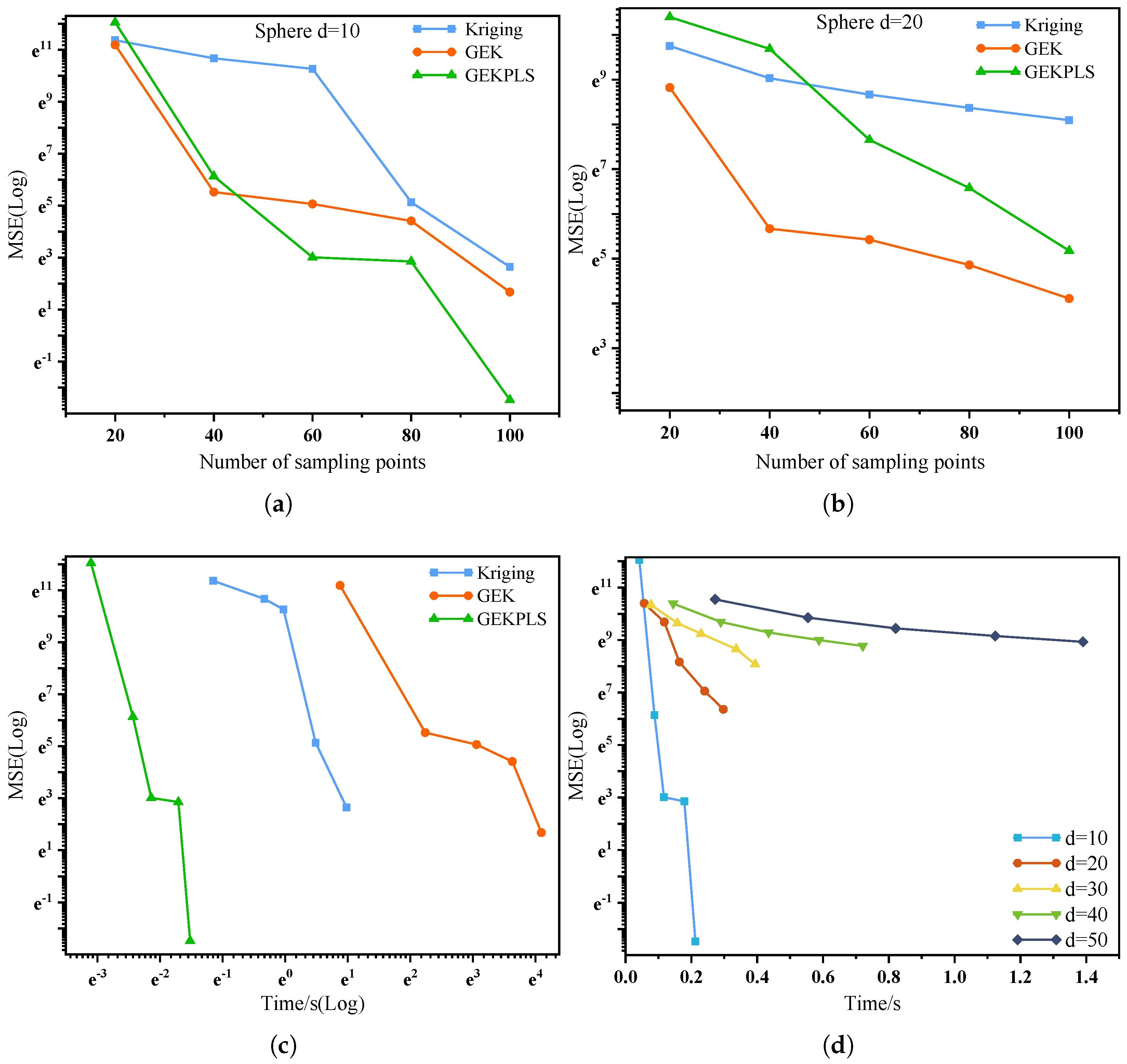
2.3. Gradient-Enhanced Kriging with Partial Least Squares Approach

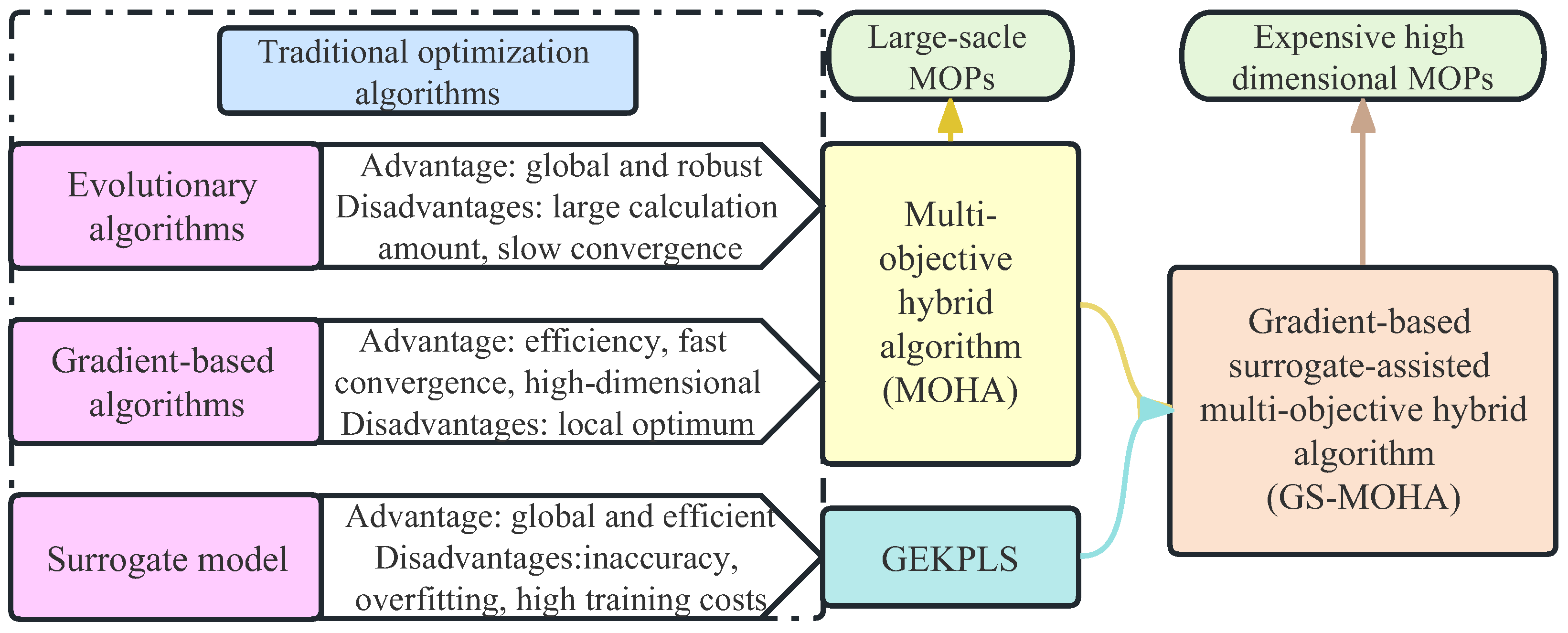
The GEK model was developed based on the Kriging model. Its principle is the same as the Kriging model. The difference is that not only the function values at the sample points but also the gradient values at the sample points are used in the training of the model. Adding gradient information can improve model training accuracy under a given number of sampling points [38]. In aerodynamic shape design, the gradient information can be easily obtained through the adjoint method. Therefore, gradient-based approximate modeling techniques are widely used and developing rapidly [39,40]. The training of the Kriging model is accomplished by solving the maximum likelihood function to determine the most suitable hyperparameters. This training process requires inverse operations on the matrices, leading to significant computational costs. Although the GEK model is more accurate than Kriging, the training efficiency still decreases rapidly as the dimensionality of the variables increases. To improve the training efficiency of high-dimensional optimization problems, the partial least squares (PLS) method is adopted in the GEK model to simplify the problem and establish the GEKPLS model [29]. It is a surrogate modeling method that leverages gradient information to achieve greater accuracy with fewer hyperparameters in high-dimensional problems. This method generates a set of approximating points using the first-order Taylor approximation method around each sampling point. The local influence of each vector space is then determined through several applications of the PLS method. Moreover, the global impact on the output function is obtained by calculating the average of all PLS coefficients. In essence, GEKPLS can reduce the hyperparameters and slightly increase the size of the correlation matrix, thus requiring fewer computational resources.

The global PLS coefficient is $w^{\left(l\right)}=[w_1^l,\cdots ,w_d^l],l=1,\cdots ,h$, d is the input dimension of the original problem, and h is the number of principal component vectors in the PLS method. To construct the GEKPLS Gaussian kernel, we first define the linear map $F_l$ via:

$$\begin{array}{cc}\hfill F_l:B& ⟶B\hfill \\ \hfill \mathbf{x}& ⟼\left[w_{{\mathrm{v}}_1}^{\left(l\right)}{x}_1,\dots ,w_{{\mathrm{v}}_d}^{\left(l\right)}{x}_d\right]\hfill \end{array}$$

(3)

Then, we build the GEKPLS kernel:

$$k\left(\mathrm{x},{\mathrm{x}}^{\prime }\right)={\sigma }^2\prod _{l=1}^h\prod _{i=1}^{d}exp\left[-{\theta }_l{\left(w_{v_i}^{\left(l\right)}{x}_i-w_{v_i}^{\left(l\right)}{x}_i^{\prime }\right)}^2\right],\forall {\theta }_l\in [0,+\infty ),\forall \mathrm{x},{\mathrm{x}}^{\prime }\in B$$

(4)

where B is a hypercube represented by the product of each vector space interval. This approach reduces the number of hyperparameters from d to h, where $h<<d$. In practical applications, h generally takes 1–3, thus significantly reducing the time to construct the model. More details of this approach are given by [29,41].

Take the multivariate sphere function as an example:

$$f\left(x\right)=\sum _{i=1}^d{x}_i^2,-10\le x_i\le 10,i=1,\dots ,d$$

(5)

To evaluate the errors of different surrogate models, we calculate the mean square error (MSE) using the following equation:

$$MSE=\frac{1}{n}\sum _{i=1}^n{(f_i-y_i)}^2$$

(6)

where $f_i$ and $y_i$ represent the real value of the sample points and their corresponding predicted values and n is the number of sample points. We use Kriging, indirect GEK, and GEKPLS methods to build the surrogate model, respectively. The sample points are increased from $n=20$ to $n=100$ with an interval of 20. But we use $2n$ sampling points for each case in the Kriging model. Since the Kriging model cannot utilize the gradient information, the gradient computation time is replaced by increasing the number of function calculations. Moreover, we change the dimension of the sphere function from d = 10 to d = 50 with an increment of 10.

As shown in Figure 4, the GEK and GEKPLS models based on gradient information are more accurate than traditional Kriging in most cases, but the training time of GEK models is longer. For example, in Figure 4c, when $N=100$ and $d=10$, the GEK model training time is 60.4 s, while GEKPLS takes only 0.3 s. Furthermore, we compare the training time of GEKPLS in different dimensions, as shown in Figure 4d. In the sphere function with up to 50 dimensions, the GEKPLS model completed the training of 100 sample points in less than 2 s, demonstrating high efficiency. The GEKPKS model is able to construct an accurate Kriging model for high-dimensional problems using gradient information at sampling points. This method solves the issues of the ordinary Kriging model, which has a large and dense correlation matrix. For high-dimensional problems, the training time for the model is often much longer than the CFD analysis time, making it difficult to apply to aerodynamic optimization problems with 30 dimensions or more. Therefore, it can be ascertained that GEKPLS shows good performance in the domains of training time as well as accuracy. The aforementioned benefits are indeed alluring in the context of engineering applications.

2.4. Motivation

EAs attain global optimization for diverse problem typologies, inclusive of continuous and discontinuous, convex and non-convex, and unimodal and multimodal ones, via the curation of superior genetic sequences through selection, recombination, and mutation. However, EAs require a large population size and numerous fitness evaluations to find the global optimum solution, and their convergence speed is relatively slow. Therefore, to improve the optimization speed, GBAs are a commonly used approach. GBAs need initial points that are close to the optimal solution to reach the global optimum during convergence. Additionally, the algorithm has the potential to converge towards a local optimum rather than the global optimum and is sensitive to the initial conditions. Both algorithms have their advantages and limitations but remain widely used in the field of aerodynamic optimization. Hybrid algorithms combining EAs and GBAs have been successfully applied to the single objective aerodynamic shape optimization of a fore body of a hypersonic air-breathing vehicle [42].

In complex aerodynamic shape design, we often encounter high-dimensional aerodynamic optimization problems with many decision variables ($D>10$) for multiple objectives and disciplines, as shown in Figure 5. Currently, we mainly use adjoint methods to solve large-scale optimization problems. For high-dimensional multi-objective aerodynamic optimization problems, MOEAs can be used in addition to the weighted sum method for solving. But most existing MOEAs need multiple iterations to search for the PFs, making them inefficient and unacceptable.

To alleviate this problem, it is necessary to improve the efficiency of optimization in two respects: (1) the search efficiency of multi-objective optimization algorithms, and (2) the efficiency of CFD analysis in aerodynamics. Therefore, it is highly attractive to propose an efficient multi-objective algorithm if it can solve large-scale aerodynamic optimization problems while reducing expensive CFD calculations.

Based on the above, we present two optimization algorithms: MOHA and GS-MOHA. The former is a hybrid multi-objective optimization algorithm based on global evolution and local gradient search. It makes full use of the advantages of gradient algorithm and evolutionary algorithm to improve the efficiency of MOEA. The latter is an efficient generalization of MOHA combined with the GEKPLS model under a hybrid framework to solve the expensive CFD analysis. Their biggest difference is that GS-MOHA is a surrogate-assisted algorithm that replaces expensive CFD calculations through surrogate models. GS-MOHA requires fewer true evaluations than MOHA when solving the same optimization problem.

The proposed algorithm process in this paper is shown in Figure 6. MOHA is the core algorithm in this framework, and its main idea is to accelerate the evolution process of MOEA through the multi-objective local gradient search algorithm. In addition, aerodynamic shape design often faces the problems of many design variables and long CFD simulation time. Therefore, combining the GEKPLS model with a hybrid algorithmic framework overcomes the disadvantages of slow algorithm convergence and long model training time in high-dimensional global optimization.

3. Hybrid Multi-Objective Algorithm Coupling Global Evolution and Local Gradient Search

In this section, we design a reasonable hybrid framework that balances the algorithm’s global exploitation and local exploration capabilities. In the hybrid framework, MOHA is proposed, which not only improves the convergence speed of the algorithm but also maintains population diversity.

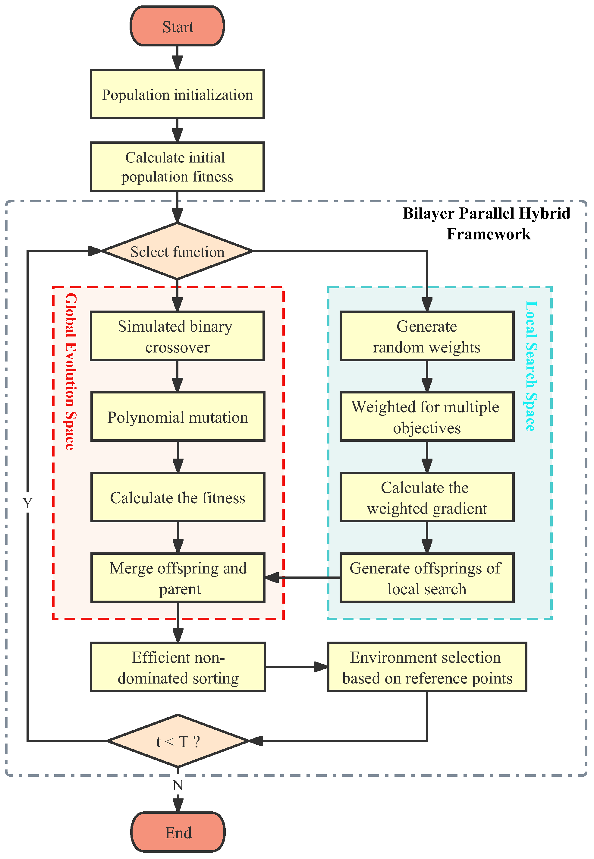
3.1. Hybrid Multi-Objective Algorithm Framework

As explicated in Section 2.1, the MOEAs exhibit robust global search capabilities. As the number of objectives and decision variables increase, these algorithms encounter a significant decline in their convergence pressure. Consequently, achieving convergence of the algorithm becomes a formidable task. Dominance-based MOEAs are known to have notable shortcomings when it comes to their capacity to attain the real PF. This is particularly true when the objective value is in proximity to the PF because oscillations may arise. The oscillation of the MOEA solution set can be attenuated by implementing local gradient search techniques [13,43]. Figure 7 shows that by combining local search techniques with the results of MOEA, the convergence pressure of the algorithm is enhanced and the solution set is closer to the true PF. GBAs can provide sufficient convergence pressure on the population, allowing them to converge faster to the PF. Consequently, local search methods can facilitate EAs in generating solutions that effectively approximate the true PF. Research indicates that incorporating additional information into the process of evolution, such as gradient search techniques and special combination operators, can greatly improve the search efficiency and solution accuracy of MOEAs [13,44,45,46].

Currently, most hybrid algorithms use local search techniques after the evolution of MOEA is completed or alternate local search methods during the run of the algorithm [47]. Engaging in a local search predicated on gradient information for all individuals during the algorithm’s iteration not only necessitates a substantial computation cost but also culminates in the premature convergence of the algorithm. Inspired by the literature [42] and [48], a bilayer parallel hybrid algorithm framework based on multi-objective gradient search techniques is proposed in this paper, as presented in Figure 8.

The hybrid algorithm framework exhibits a parallel mechanism characterized by a bilayer spatial configuration. This design displays remarkable flexibility and scalability properties. Therefore, any MOEA and local search algorithm can be used in this framework. To be specific, crossover and mutation operations are executed to generate offspring in the global evolution space in MOHA. Meanwhile, using the MOGBA as proposed in Section 2.2 for gradient search within the local search space has facilitated the evolution of the population and greatly improved the efficiency of the algorithm. Furthermore, the employment of the same environmental selection mechanism as NSGA-III by MOHA has led to the increased diversity of non-dominated solutions through the application of well-distributed reference vectors to select new parent solutions. This hybrid strategy makes full use of the global optimization capability of MOEA and the local convergence efficiency of MOGBA.

Through the inheritance and interaction of these two spaces, the diversity and convergence of the algorithm population are balanced. As a consequence, the proposed MOHA improves convergence while maintaining favorable diversity. Algorithm 2 presents the details of MOHA, which is an efficient multi-objective optimization algorithm for solving large-scale MOPs.

First, the global and local spaces are initialized according to the population size N and initial acceptance probability P. The global space performs global evolution through genetic operators, while the local space performs a multi-objective gradient search, which operates in parallel, and the respective populations update themselves to generate offspring. In the main loop, the number of individuals entering the local space is controlled by the dynamic selection function. Each iteration selects $n_{accept}$ elite individuals into the local space by using Equation (7). Then, the individuals after the gradient search are injected into the global evolution space for individual migration interactions. By introducing new genes, the diversity and convergence of the population can be promoted, thereby improving the performance of the algorithm. Then, the original population and the newly generated offspring are merged, and the non-dominated sort operation is performed on $R_t$. Finally, use the environment selection mechanism to select new individuals for the next iteration. The algorithm terminates until the maximum iteration number T is reached. The dynamic selection function is:

$$n_{accept}=[(P+\frac{P}{t})\times N]$$

(7)

Note that the brackets represent a Gaussian function, also known as a rounding function; t is the current evolution generation; and P controls the number of individuals that go into the local search space. With the utilization of the dynamic acceptance function, it is possible to regulate the influx of individuals entering the local space by ensuring a higher number in the initial stages of algorithm iteration and subsequently decrease their number later on. As a result, the diversity and convergence of populations can be better balanced.

Algorithm 2 MOHA Procedure
Input: N (population size), $P_c$ (crossover probability), $P_m$ (mutation probability), T (maximum iteration number), P (acceptance probability), M (number of objectives) Output: $Q_{t+1}$ (next population)
1:	t ← 0;
2:	Z ← $ReferencePointsGeneration\left(M\right);$
3:	$P_t$ ← $GlobalSpaceInitialization\left(\right);$
4:	$P_b$ ← $LocalSpaceInitialization\left(\right);$
5:	while $t<T$ do
6:	$N_{accept}$←$AcceptanceFunction\left(P\right);$
7:	if Local search then
8:	for $j=1\to N_{accept}$ do
9:	$Q_b$ ← $Algorithm1\left(P_b\right)$; //Local search based on gradient information
10:	end for
11:	$F_t$ ← $NondominatedSort$ ($Q_b$∪$P_b$);
12:	else
13:	$Q_t$ ← $GeneticOperation$ ($P_t$,$P_c$,$P_m$);//Global search
14:	end if
15:	$R_t$ ← $F_t$∪$Q_t$;
16:	($F_1,F_2,\cdots$) ← $NondominatedSort$ ($R_t$);
17:	$S_t$ ← Ø, i ← 1;
18:	repeat
19:	$S_t$ ← $S_t$∪$F_i$ and i ← i + 1
20:	until $|S_t|\ge N$
21:	Last front to be included: $F_l$ = $F_i$;
22:	if $|S_t|=N$ then
23:	$P_{t+1}$=$S_t$, break
24:	else
25:	$Q_{t+1}$ = ${\bigcup }_{j=1}^{l-1}{F}_j$;
26:	$Z^r\leftarrow Normalize(Z,S_t);$          //$Z^r$:reference points on normalized hyperplane
27:	Points to be chosen from $F_l$: $K=N-|Q_{t+1}|$;
28:	[$\pi \left(s\right),d\left(s\right)$] ← $Associate$ ($S_t,Z^r$); // $\pi \left(s\right)$:closest reference point, d:distance between s and $\pi \left(s\right)$
29:	$Q_{t+1}$ ← $Niching$ ($K,{\rho }_j,\pi ,d,Z,F_l,Q_{t+1}$);//${\rho }_j$:niche count for the jth reference point
30:	end if
31:	t ← $t+1$
32:	end while

3.2. Sensitivity Analysis of the Local Search Parameter P

To verify the efficiency of the developed hybrid framework and the influence law of the multi-objective gradient search mechanism on MOEA, a sensitivity analysis was carried out on the parameter P. Here, we still take DTLZ2 as an example, and the number of iterations is set to 30 generations. We do this because a smaller number of iterations can more clearly compare the difference between the algorithm under different P. Figure 9 shows the influence of the local search frequency P on the convergence performance of the algorithm. The convergence speed of the algorithm will become increasingly faster when P changes from 0 to 0.4. If the value of P is too large, the computational cost of the algorithm will increase. The algorithm degenerates to an ordinary MOEA at $P=0$. At this moment, the convergence is the slowest and the search efficiency also is the lowest. With the increase in P, the more individuals are selected into the local search space, the faster the algorithm converges. However, this promotion effect non-linearly increases. For example, after $p>0.1$, the search efficiency improves very slowly. Moreover, even with a very small value such as $P=0.01$ is still very significant for improving the search efficiency of MOEA, which demonstrates the rationality and efficiency of the hybrid algorithm framework. The solution generated by the MOGBA can guide MOEA to approach the PF fast. In summary, the MOHA algorithm selects elite individuals in the local search space with a probability of $P=0.1$ during the iterations and only performs one gradient iteration each time. Finally, the individuals after the local search and the global search are mixed to generate new offspring, which produces new knowledge and increases the diversity of the population.

3.3. Population Evolution and Acceleration Mechanism Analysis of Multi-Objective Hybrid Algorithm

Figure 10 illustrates the variation process of the approximate PF distribution for the three algorithms on ZDT2 [33]. According to Figure 10, discovering the approximate PF through MOEA requires about 100 generations of evolution. In contrast, MOGBA and MOHA are capable of finding the optimal PF in only 10 iterations. Obviously, the convergence efficiency of MOGBA and MOHA is about 10 times higher than that of MOEA, while the efficiency of MOGBA and MOHA is similar. Moreover, ZDT2 is a non-convex function and MOGBA can still solve it very well, further proving that our improvement of the gradient algorithm is reasonable and feasible. By comparing Figure 10b,c, the proposed MOHA also has better diversity than MOGBA while maintaining high convergence. As demonstrated, hybrid algorithms are not simply the combination of two algorithms. The advantages of hybrid algorithms lie in their ability to leverage the strengths of each algorithm while avoiding their weaknesses. The acceleration mechanisms of MOHA are analyzed as follows:

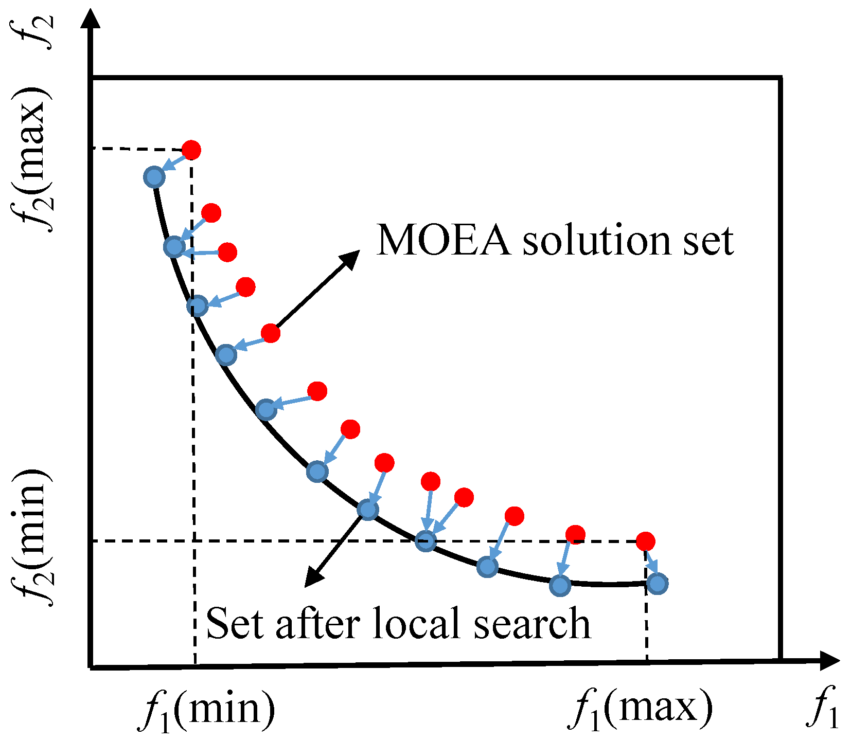
• In the hybrid framework, elite individuals are selected into the local space. These elite individuals are generated by MOEA and carry the vast majority of useful information. A multi-objective gradient search on this basis not only amplifies this advantage but also increases population diversity.
• The quality of most offspring solutions generated by local search is always better than that of global search as shown by the red dots in Figure 10c. They carry a great number of excellent genes and a great deal of knowledge and are therefore able to guide the evolutionary direction of other individuals. This information exchange substantially improves the speed of the algorithm in finding the global optimal solution.
• The proposed algorithm can quickly approximate the global optimal PF, mainly due to its good global exploration and local search capabilities. When MOEA approaches the true Pareto front, it tends to slow down and the solutions generated may oscillate. This phenomenon can be eliminated by using hybridization.

The above three mechanisms work together synergistically to produce an accelerated convergence effect that improves algorithm performance significantly. It is these acceleration mechanisms of the hybrid algorithm that make it possible to solve large-scale MOPs.

4. Hybrid Optimization Algorithm Based on GEKPLS Surrogate Model

The proposed MOHA, as presented in the preceding section, enhances the search proficiency of the algorithm. This section aims to further enhance the optimization efficiency of the hybrid algorithm by tackling the issue of costly fitness assessment in engineering optimization. Thus, we have proposed the GS-MOHA, which employs the GEKPLS surrogate model to approximate costly fitness calculations. The algorithm takes full advantage of the scalability of the hybrid algorithmic framework. The gradient information generated in the local search space not only promotes population convergence but also improves the accuracy of the surrogate model. Overall, GS-MOHA has enhanced the engineering applicability of MOHA for complex aerodynamic shape optimization in aircraft.

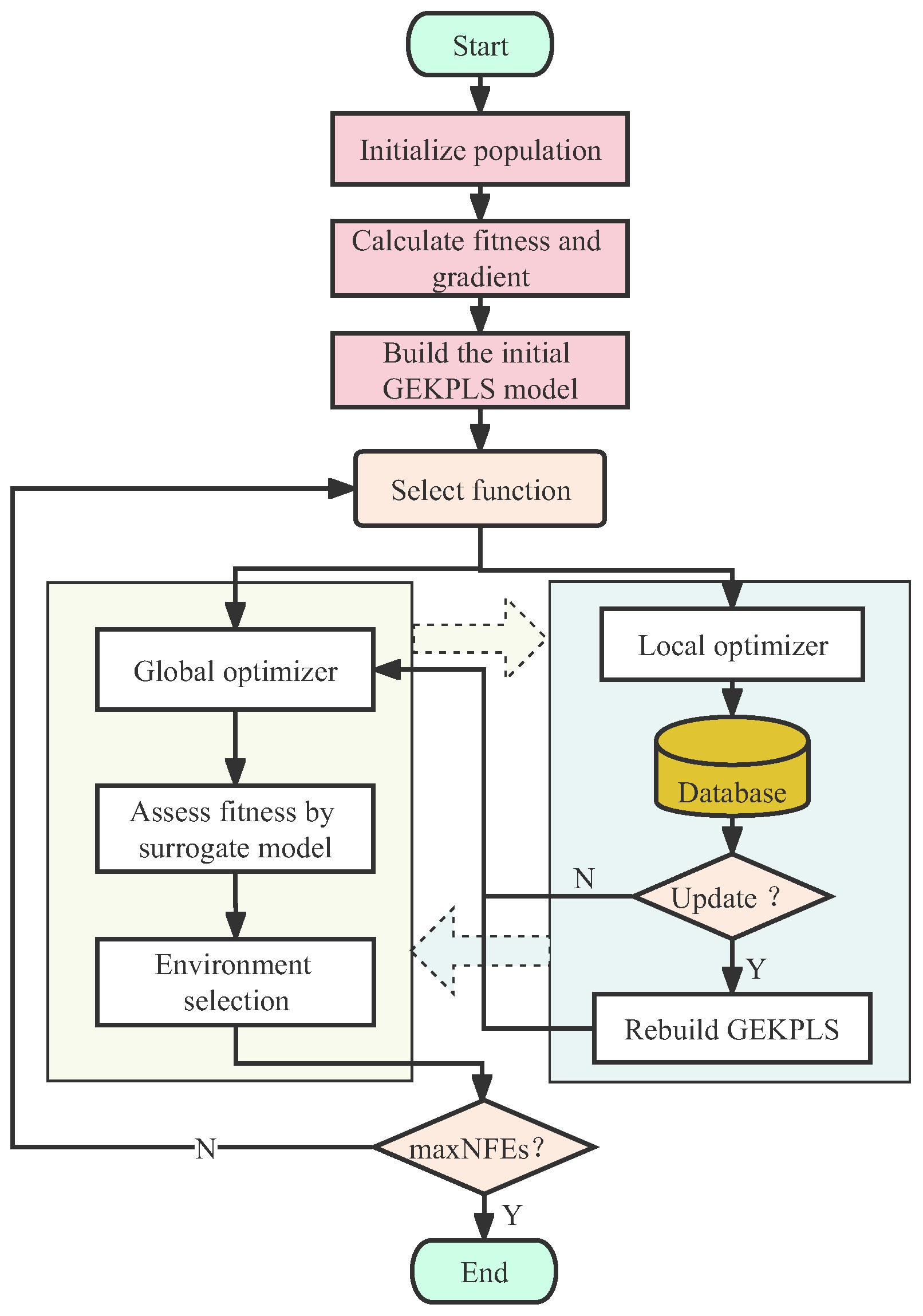
4.1. Surrogate-Assisted Hybrid Multi-Objective Algorithm Framework

In this section, we present the details of GS-MOHA proposed for solving expensive MOPs. GS-MOHA uses both surrogate-assisted global search strategies and local search update strategies to improve the optimization efficiency of MOHA. The optimization framework of GS-MOHA is plotted in Figure 11, which is similar to the MOHA framework.

To fully utilize data and save time, GS-MOHA maintains a similar framework to MOHA. The efficiency and simplicity of the hybrid algorithm framework are inherited. GS-MOHA consists of three main components: (1) global optimizer; (2) local optimizer; (3) GEKPLS surrogate model. Specifically, MOEA and MOGBA are employed as global and local optimizers, respectively, to strike a balance between global exploration and local exploitation capabilities. Unlike MOHA, we embed the GEKPLS model into the hybrid framework to reduce the number of expensive fitness evaluations. The numerical implementation of GS-MOHA is expounded in a step-by-step manner as follows:

• Step 1: Generate random populations and evaluate their objective function values and gradient values. After that, the initial surrogate model of GEKPLS is built.
• Step 2: Control the global evolution and local search behaviors of individuals using selection functions. The global optimizer uses a surrogate model for fitness calculation. The global search of the surrogate model is performed using polynomial mutation (PM) and simulated binary crossover (SBX) operators. Meanwhile, the real fitness and gradient of individuals entering the local optimizer are calculated.
• Step 3: An external database is created to store the real fitness and gradient information generated by the local optimizer in each iteration. Here, the gradient is calculated using the finite difference method, but the adjoint method is used in aerodynamic optimization.
• Step 4: Decide whether the GEKPLS model needs to be updated. If the surrogate model is updated, the GEKPLS model is rebuilt with the individual information from the external archive set. Otherwise, the original model is used for function evaluation.
• Step 5: Merging the offspring generated by the global and local optimizers. Then, the next generation population is selected through the environmental selection mechanism.
• Step 6: Stop the algorithm if the stopping criterion is satisfied. Otherwise, go to Step 2.

The proposed GS-MOHA has four significant merits:

(1)

With MOHA as the main driving engine, GS-MOHA inherits all the advantages of the hybrid algorithm and has a faster convergence speed.

(2)

Combining fitness values and gradient values at each sampling point has the potential to enrich the surrogate model. This means that GS-MOHA runs faster and with higher accuracy for the same number of sampling points. The local search technique based on gradient information not only facilitates the evolution of the population but also enhances the quality of the surrogate model.

(3)

GS-MOHA uses a multi-point infill strategy. The number of filling points is related to the number of elite solutions in local search. This infill strategy makes reasonable and efficient use of the hybrid algorithm framework.

(4)

GS-MOHA is capable of solving expensive MOPs with decision variable dimensions greater than 10. Due to the adoption of the GEKPLS and hybrid algorithm framework, the search efficiency and modeling accuracy in high-dimensional design spaces are better than traditional methods. This fulfills our primary purpose of pursuing efficiency in engineering optimization.

4.2. Model Update Management and Validation

In SAEA, model management is a very important strategy that controls the update of the surrogate model and has a great influence on the optimization results. A good model management strategy can guide the algorithm to converge to the global optimum faster, while a bad model management strategy is just the opposite. Currently, the expected improvement (EI) criterion based on the uncertainty of the predicted value is the most common. But when extended to high-dimensional multi-objective optimization, the formula becomes more complicated and only one new point can be added each time [25,26]. Other management strategies such as the probability of improvement (PI) criterion, surrogate-based optimization (SBO) criterion, and lower confidence bound (LCB) criterion are also widely used in SAEA [49,50,51]. The role of the surrogate model in SBO has changed. It is no longer a simple substitution role but constitutes an optimization mechanism based on historical data to drive sample point addition and thus the approximation of locally or globally optimal solutions. This approach is particularly suitable for multi-objective optimization. Because this method can add points in batches around PF, it focuses on high-precision surrogate modeling in the local area where the optimal solution is located rather than approximating the global space.

Algorithm 3 presents the update strategy of the GEKPLS model. Firstly, a population is randomly generated and its fitness values and gradients are calculated. Then, an initial GEKPLS surrogate model is established for each objective using the fitness values and gradient values. Next, $n_{accept}$ individuals are selected for local search using the selection function. The fitness values and gradient information of the offspring generated after the local search are saved to the external archive set, while the redundant solutions are removed. Eventually, the GEKPLS model is updated when the update conditions are satisfied. Otherwise, a global search is executed on the original model.

With the iteration of the algorithm, the solution after local search becomes closer and closer to the real PF, thus improving the accuracy of the GEKPLS model fitting the space near the PF. It is worth noting that the acceptance probability is $P=0.1$ in MOHA, while the recommended value range in the GS-MOHA is (0.01, 0.05), which is set to $P=0.02$ in this paper. The reason for this is that GS-MOHA is a surrogate-based optimization algorithm to reduce expensive CFD calculations in aerodynamic shape design. The utility of GEKPLS is mainly to replace the fitness calculations of the global optimizer with a larger population size, while the small number of children generated by the local optimizer is mainly used to update the model. Therefore, the number of individuals accessing the local space must be limited, and larger values of P increase the number of expensive fitness evaluations. Although local search techniques can improve the efficiency of the algorithm, this improvement is much smaller than the CFD computational cost. Moreover, a larger P value leads to too many individuals stored in the archive set and more redundant solutions, increasing the cost of training the model. After comprehensive consideration, GS-MOHA abandons the best acceptance probability in MOHA. The cost of doing so is a slight reduction in the effectiveness of the gradient operator, but it improves the overall performance of the algorithm.

Algorithm 3 The Surrogate-Assisted Model Update Strategy
Input: P (current population), M (number of objectives), V (decision variables), K (update frequency), T (maximum number of iterations) Output: $Q_e$ (offspring population of MOEA), $Q_g$ (offspring population of MOGBA), Q (next population)
1:	Y ← $PopulationInitialization\left(V\right)$;
2:	G ← $GradientInitialization\left(V\right)$;
3:	for $i=1:M$ do
4:	$Y_i$ ← the ith column of Y;
5:	$G_i$ ← the ith column of G;
6:	GEKPLS ← $BuildSurrogateModel(V,Y_i,G_i)$;
7:	end for
8:	for $j<T$ do
9:	if $j>0$ and $j/K==0$ then
10:	Update GEKPLS with the solutions generated by Algorithm 1;
11:	else
12:	$Q_e$ ← Predicted objective values by the ith GEKPLS model;
13:	$Q_g$ ← Algorithm 1;
14:	Q ← $Q_e$∪$Q_g$;
15:	$P_{t+1}$ ← $EnvironmentalSelection\left(Q\right)$;
16:	end if
17:	end for

The update frequency K has a significant impact on the performance of GS-MOHA. Nonetheless, there is still a lack of strict frequency adjustment criteria, and we usually set them empirically. Note that if K is too small, it increases the computation time of the algorithm and cannot fully explore the surrogate model; if K is too large, the search direction may deviate from the optimal solution due to the low accuracy of the surrogate model. To choose a reasonable update frequency, this section tests the DTLZ2 and DTLZ7 functions. DTLZ2 is a continuous concave function, while DTLZ7 is a discontinuous multimodal function, which can be a good test of the performance of the algorithm. We vary the update frequency from $K=5$ to $K=20$ in increments of 5. The number of true fitness evaluations is set to 300, and the algorithm is run 20 times independently. Figure 12 presents a comparison of the algorithm performance. When $K=10$, the algorithm has the smallest average IGD metric on DTLZ2 and DTLZ7, followed by $K=15$. Compared to other operating conditions, the data fluctuation range is smaller; therefore, the algorithm has the best performance. In addition, multiple outliers appeared at $K=5$, which may be caused by frequent model updates resulting in changing search directions. Overall, the recommended value of K is 10.

5. Numerical Experiments and Discussion

In this section, comparative experiments are conducted between MOHA and four state-of-the-art MOEAs, including MOEA/D [52], NSGA-III [36], RVEA [53], and VaEA [54]. Then, we compare GS-MOHA with two SAEAs (MOEA/D-EGO [26] and K-RVEA [27]) on the DTLZ [33] problems. Furthermore, we also analyze the efficiency and scalability of MOHA and GS-MOHA.

5.1. Performance Comparison between MOHA and Existing MOEAs

5.1.1. Experimental Setting

The algorithms are tested with DTLZ problems (DTLZ1-DTLZ7), which are well known for their scalability in decision space and objective space. Notably, we change the dimensionality of the decision variables and the number of objectives of the benchmark test function.

Table 1. Test problems and characteristics.

Problems	Features
DTLZ1	Linear, multi-modal
DTLZ3	Non-convex, multi-modal
DTLZ2,4	Non-convex, unimodal
DTLZ5,6	Non-convex, degenerate PF
DTLZ7	Mixed, disconnected, and multi-modal

provides the test functions and their features. To ensure a fair comparison, all of the algorithms are evaluated using prescribed parameter values to achieve optimal performance. This study conducted all tests on a computer with an Intel^® Core^TM i7-10700K 3.80 GHz processor and 32 G memory. The parameter settings used in all of the experiments are listed below.

(1)

Population Sizing: The population size of NSGA-III and MOEA/D is not arbitrarily specified but depends on the number of reference points or weight vectors. As recommended in [55], the population size is set at 105 when $M=3$ and 126 for the corresponding $M=5$.

(2)

Termination Conditions: An increase in the number of decision variables and objective functions will increase the optimization difficulty. For the three-objective test problems, with 30 and 50 decision variables, the maximum number of evaluations is set to 50,000 and 100,000. Similarly, when $M=5$, the evaluations are set to 100,000 and 150,000, respectively. Statistical results of all test problems were obtained by 20 independent experiments for each algorithm.

(3)

Performance Metrics: The performances of the algorithms are evaluated with IGD [37] and hypervolume (HV) [46]. In principle, both IGD and HV can evaluate the convergence and diversity of the obtained non-dominated solutions. A smaller value of IGD indicates a better quality of the obtained solution set, while HV is just the opposite: a larger value indicates better solution quality.

(4)

Control parameters: For the MOHA, the acceptance probability is set to $P=0.1$. And the gradient is estimated using a 2-point finite difference estimation with an absolute step size. The number of local gradient searches is set to one. All of the algorithms adopt the same evolutionary operators such as PM and SBX. The parameters of the evolutionary operator are consistent with the literature [55].

5.1.2. Discussion of Results

The statistical IGD and HV results of different algorithms are listed in

Table 2. IGD metric values of five algorithms on DTLZ problems, where the best result on each test problem is displayed in black and bold. (“+, −, =” indicate that the result is significantly better, significantly worse, and statistically similar to that of MOHA, respectively).

Problem	M	D	MOEA/D	NSGA-III	RVEA	VaEA	MOHA
DTLZ1	3	30	$2.1856\times {10}^0$ ($1.43\times {10}^0$) −	$8.1406\times {10}^{-1}$ ($6.33\times {10}^{-1}$) −	$1.5151\times {10}^0$ ($8.10\times {10}^{-1}$) −	$7.4534\times {10}^{-1}$ ($4.88\times {10}^{-1}$) −	$\mathbf{2}.\mathbf{0561}\times {\mathbf{10}}^{-\mathbf{2}}(\mathbf{2}.\mathbf{47}\times {\mathbf{10}}^{-\mathbf{5}})$
	3	50	$2.3154\times {10}^1$ ($8.26\times {10}^0$) −	$1.3432\times {10}^1$ ($4.21\times {10}^0$) −	$1.7094\times {10}^1$ ($4.79\times {10}^0$) −	$1.4645\times {10}^1$ ($3.83\times {10}^0$) −	$\mathbf{2}.\mathbf{0662}\times {\mathbf{10}}^{-\mathbf{2}}(\mathbf{1}.\mathbf{29}\times {\mathbf{10}}^{-\mathbf{5}})$
	5	30	$4.6352\times {10}^0$ ($1.91\times {10}^0$) −	$5.0216\times {10}^0$ ($1.65\times {10}^0$) −	$2.0707\times {10}^0$ ($1.13\times {10}^0$) −	$9.2347\times {10}^0$ ($4.52\times {10}^0$) −	$\mathbf{6}.\mathbf{4905}\times {\mathbf{10}}^{-\mathbf{2}}(\mathbf{8}.\mathbf{29}\times {\mathbf{10}}^{-\mathbf{5}})$
	5	50	$3.2270\times {10}^1$ ($8.18\times {10}^0$) −	$3.1468\times {10}^1$ ($6.19\times {10}^0$) −	$1.8731\times {10}^0$ ($4.58\times {10}^0$) −	$4.2893\times {10}^1$ ($1.05\times {10}^1$) −	$\mathbf{6}.\mathbf{8126}\times {\mathbf{10}}^{-\mathbf{2}}(\mathbf{1}.\mathbf{27}\times {\mathbf{10}}^{-\mathbf{4}})$
DTLZ2	3	30	$5.4464\times {10}^{-2}$ ($1.92\times {10}^{-7}$) =	$5.4465\times {10}^{-2}$ ($6.63\times {10}^{-7}$) −	$5.4464\times {10}^{-2}$ ($6.91\times {10}^{-7}$) −	$5.8066\times {10}^{-2}$ ($8.02\times {10}^{-4}$) −	$\mathbf{5}.\mathbf{3612}\times {\mathbf{10}}^{-\mathbf{2}}(\mathbf{4}.\mathbf{69}\times {\mathbf{10}}^{-\mathbf{7}})$
	3	50	$5.4467\times {10}^{-2}$ ($8.48\times {10}^{-7}$) −	$5.4468\times {10}^{-2}$ ($2.02\times {10}^{-6}$) −	$5.4466\times {10}^{-2}$ ($8.20\times {10}^{-7}$) −	$5.8108\times {10}^{-2}$ ($8.67\times {10}^{-4}$) −	$\mathbf{5}.\mathbf{3634}\times {\mathbf{10}}^{-\mathbf{2}}(\mathbf{6}.\mathbf{72}\times {\mathbf{10}}^{-\mathbf{7}})$
	5	30	$\mathbf{2}.\mathbf{1205}\times {\mathbf{10}}^{-\mathbf{1}}(\mathbf{1}.\mathbf{09}\times {\mathbf{10}}^{-\mathbf{4}})+$	$2.1223\times {10}^{-1}$ ($2.87\times {10}^{-5}$) −	$2.1222\times {10}^{-1}$ ($5.79\times {10}^{-6}$) −	$2.1653\times {10}^{-1}$ ($1.46\times {10}^{-3}$) −	$2.1220\times {10}^{-1}$ ($1.73\times {10}^{-5}$)
	5	50	$\mathbf{2}.\mathbf{1209}\times {\mathbf{10}}^{-\mathbf{1}}(\mathbf{1}.\mathbf{01}\times {\mathbf{10}}^{-\mathbf{4}})+$	$2.1227\times {10}^{-1}$ ($1.24\times {10}^{-5}$) −	$2.1224\times {10}^{-1}$ ($9.02\times {10}^{-6}$) −	$2.1737\times {10}^{-1}$ ($1.20\times {10}^{-3}$) −	$2.1311\times {10}^{-1}$ ($1.65\times {10}^{-5}$)
DTLZ3	3	30	$8.6438\times {10}^0$ ($4.97\times {10}^0$) −	$1.1698\times {10}^0$ ($9.57\times {10}^{-1}$) −	$6.3482\times {10}^0$ ($3.53\times {10}^0$) −	$1.6131\times {10}^0$ ($1.40\times {10}^0$) −	$\mathbf{5}.\mathbf{4491}\times {\mathbf{10}}^{-\mathbf{2}}(\mathbf{1}.\mathbf{16}\times {\mathbf{10}}^{-\mathbf{6}})$
	3	50	$7.9663\times {10}^1$ ($2.14\times {10}^1$) −	$3.3094\times {10}^1$ ($7.37\times {10}^0$) −	$6.5109\times {10}^1$ ($1.86\times {10}^1$) −	$3.3455\times {10}^1$ ($8.32\times {10}^0$) −	$\mathbf{5}.\mathbf{4493}\times {\mathbf{10}}^{-\mathbf{2}}(\mathbf{1}.\mathbf{06}\times {\mathbf{10}}^{-\mathbf{6}})$
	5	30	$1.9898\times {10}^1$ ($1.05\times {10}^1$) −	$1.4293\times {10}^1$ ($5.88\times {10}^0$) −	$7.2137\times {10}^0$ ($3.69\times {10}^0$) −	$2.4082\times {10}^1$ ($9.36\times {10}^0$) −	$\mathbf{2}.\mathbf{1790}\times {\mathbf{10}}^{-\mathbf{1}}(\mathbf{1}.\mathbf{27}\times {\mathbf{10}}^{-\mathbf{2}})$
	5	50	$1.2696\times {10}^2(3.01\times {10}^1)$−	$1.0811\times {10}^2(2.69\times {10}^1)$−	$7.6486\times {10}^1(2.17\times {10}^1)$−	$1.5170\times {10}^2(3.63\times {10}^1)$−	$\mathbf{2}.\mathbf{2840}\times {\mathbf{10}}^{-\mathbf{1}}(\mathbf{1}.\mathbf{86}\times {\mathbf{10}}^{-\mathbf{2}})$
DTLZ4	3	30	$3.9787\times {10}^{-1}(3.36\times {10}^{-1})$−	$1.8436\times {10}^{-1}(2.19\times {10}^{-1})$−	$\mathbf{5}.\mathbf{4464}\times {\mathbf{10}}^{-\mathbf{2}}(\mathbf{8}.\mathbf{32}\times {\mathbf{10}}^{-\mathbf{7}})+$	$5.8094\times {10}^{-2}(5.81\times {10}^{-4})$−	$5.4465\times {10}^{-2}(8.49\times {10}^{-7})$
	3	50	$5.5993\times {10}^{-1}(3.57\times {10}^{-1})$−	$2.0060\times {10}^{-1}(2.27\times {10}^{-1})-$	$5.4466\times {10}^{-2}(9.11\times {10}^{-7})=$	$8.8005\times {10}^{-2}(1.62\times {10}^{-1})-$	$\mathbf{5}.\mathbf{4465}\times {\mathbf{10}}^{-\mathbf{2}}(\mathbf{9}.\mathbf{40}\times {\mathbf{10}}^{-\mathbf{7}})$
	5	30	$5.2263\times {10}^{-1}(1.79\times {10}^{-1})-$	$2.8917\times {10}^{-1}(1.11\times {10}^{-1})-$	$2.4803\times {10}^{-1}(8.14\times {10}^{-2})-$	$2.1997\times {10}^{-1}(1.66\times {10}^{-3})-$	$\mathbf{2}.\mathbf{1225}\times {\mathbf{10}}^{-\mathbf{1}}(\mathbf{3}.\mathbf{56}\times {\mathbf{10}}^{-\mathbf{5}})$
	5	50	$6.3359\times {10}^{-1}(2.03\times {10}^{-1})-$	$2.7934\times {10}^{-1}(1.04\times {10}^{-1})-$	$2.4105\times {10}^{-1}(7.45\times {10}^{-2})-$	$2.2088\times {10}^{-1}(1.40\times {10}^{-3})-$	$\mathbf{2}.\mathbf{1226}\times {\mathbf{10}}^{-\mathbf{1}}(\mathbf{3}.\mathbf{84}\times {\mathbf{10}}^{-\mathbf{5}})$
DTLZ5	3	30	$3.3866\times {10}^{-2}(2.71\times {10}^{-5})-$	$1.3181\times {10}^{-2}(1.86\times {10}^{-3})-$	$7.4851\times {10}^{-2}(1.55\times {10}^{-2})-$	$5.5460\times {10}^{-3}(2.25\times {10}^{-4})-$	$\mathbf{4}.\mathbf{7204}\times {\mathbf{10}}^{-\mathbf{3}}(\mathbf{1}.\mathbf{48}\times {\mathbf{10}}^{-\mathbf{4}})$
	3	50	$3.3776\times {10}^{-2}(6.01\times {10}^{-5})-$	$1.4107\times {10}^{-2}(2.30\times {10}^{-3})-$	$7.5091\times {10}^{-2}(1.46\times {10}^{-2})-$	$5.5915\times {10}^{-3}(2.01e\times {10}^{-4})-$	$\mathbf{5}.\mathbf{1166}\times {\mathbf{10}}^{-\mathbf{3}}(\mathbf{4}.\mathbf{92}\mathbf{e}\times {\mathbf{10}}^{-\mathbf{4}})$
	5	30	$2.6013\times {10}^{-2}(6.13\times {10}^{-4})-$	$1.6185\times {10}^{-1}(4.28\times {10}^{-2})-$	$2.4838\times {10}^{-1}(5.28\times {10}^{-2})-$	$2.2965\times {10}^{-1}(3.80\times {10}^{-2})-$	$\mathbf{2}.\mathbf{4262}\times {\mathbf{10}}^{-\mathbf{2}}(\mathbf{3}.\mathbf{18}\times {\mathbf{10}}^{-\mathbf{4}})$
	5	50	$2.6340\times {10}^{-2}(6.08\times {10}^{-4})-$	$1.8359\times {10}^{-1}(3.51\times {10}^{-2})-$	$2.4593\times {10}^{-1}(5.66\times {10}^{-2})-$	$2.9337\times {10}^{-1}(3.02\times {10}^{-2})-$	$\mathbf{2}.\mathbf{5046}\times {\mathbf{10}}^{-\mathbf{2}}(\mathbf{5}.\mathbf{03}\times {\mathbf{10}}^{-\mathbf{4}})$
DTLZ6	3	30	$3.3884\times {10}^{-2}(4.63\times {10}^{-5})-$	$1.9484\times {10}^{-2}(2.68\times {10}^{-3})-$	$1.2542\times {10}^{-1}(2.85\times {10}^{-2})-$	$\mathbf{5}.\mathbf{1653}\times {\mathbf{10}}^{-\mathbf{3}}(\mathbf{1}.\mathbf{87}\times {\mathbf{10}}^{-\mathbf{4}})+$	$6.6196\times {10}^{-3}(2.38\times {10}^{-3})$
	3	50	$3.6268\times {10}^{-2}(5.89\times {10}^{-3})-$	$2.5487\times {10}^{-2}(9.27\times {10}^{-3})-$	$2.0971\times {10}^{-1}(2.16\times {10}^{-1})-$	$\mathbf{1}.\mathbf{3708}\times {\mathbf{10}}^{-\mathbf{2}}(\mathbf{1}.\mathbf{19}\times {\mathbf{10}}^{-\mathbf{2}})+$	$2.2452\times {10}^{-2}(1.98\times {10}^{-3})$
	5	30	$2.4153\times {10}^{-1}(1.95\times {10}^{-3})-$	$8.4383\times {10}^{-1}(2.68\times {10}^{-1})-$	$2.4051\times {10}^{-1}(5.79\times {10}^{-2})-$	$2.2215\times {10}^0(1.32\times {10}^0)-$	$\mathbf{7}.\mathbf{1353}\times {\mathbf{10}}^{-\mathbf{2}}(\mathbf{1}.\mathbf{01}\times {\mathbf{10}}^{-\mathbf{2}})$
	5	50	$2.9795\times {10}^{-1}(4.71\times {10}^{-1})-$	$3.5023\times {10}^0(1.41\times {10}^0)-$	$4.0863\times {10}^{-1}(2.84\times {10}^{-1})-$	$1.3260\times {10}^1(2.56\times {10}^0)-$	$\mathbf{7}.\mathbf{8761}\times {\mathbf{10}}^{-\mathbf{2}}(\mathbf{5}.\mathbf{30}\times {\mathbf{10}}^{-\mathbf{2}})$
DTLZ7	3	30	$1.5421\times {10}^{-1}(1.64\times {10}^{-1})-$	$7.0356\times {10}^{-2}(5.45\times {10}^{-2})-$	$1.0501\times {10}^{-1}(1.37\times {10}^{-3})-$	$6.4146\times {10}^{-2}(7.23\times {10}^{-2})-$	$\mathbf{6}.\mathbf{2330}\times {\mathbf{10}}^{-\mathbf{2}}(\mathbf{2}.\mathbf{93}\times {\mathbf{10}}^{-\mathbf{3}})$
	3	50	$1.7749\times {10}^{-1}(1.18\times {10}^{-1})-$	$7.7570\times {10}^{-2}(3.62\times {10}^{-3})-$	$1.0497\times {10}^{-1}(1.46\times {10}^{-3})-$	$\mathbf{6}.\mathbf{7215}\times {\mathbf{10}}^{-\mathbf{2}}(\mathbf{1}.\mathbf{55}\times {\mathbf{10}}^{-\mathbf{3}})+$	$6.8855\times {10}^{-2}(5.35\times {10}^{-2})$
	5	30	$1.0070\times {10}^0(2.10\times {10}^{-1})-$	$\mathbf{3}.\mathbf{7415}\times {\mathbf{10}}^{-\mathbf{1}}(\mathbf{3}.\mathbf{22}\times {\mathbf{10}}^{-\mathbf{2}})+$	$5.0679\times {10}^{-1}(5.78\times {10}^{-3})-$	$3.7955\times {10}^{-1}(1.10\times {10}^{-2})=$	$3.7962\times {10}^{-1}(7.72\times {10}^{-2})$
	5	50	$1.0737\times {10}^0(1.70\times {10}^{-1})-$	$4.0329\times {10}^{-1}(1.32\times {10}^{-2})-$	$5.0781\times {10}^{-1}(2.73\times {10}^{-3})-$	$3.8611\times {10}^{-1}(1.05\times {10}^{-2})=$	$\mathbf{3}.\mathbf{8598}\times {\mathbf{10}}^{-\mathbf{1}}(\mathbf{6}.\mathbf{37}\times {\mathbf{10}}^{-\mathbf{2}})$
+/−/=			2/25/1	1/27/0	1/26/1	3/23/2	N/A

and

Table 3. HV metric values of five algorithms on DTLZ problems, where the best result on each test problem is displayed in black and bold.

Problem	M	D	MOEA/D	NSGA-III	RVEA	VaEA	MOHA
DTLZ1	3	30	$6.4718\times {10}^{-3}(2.49\times {10}^{-2})-$	$8.4464\times {10}^{-2}(2.31\times {10}^{-1})-$	$2.6614\times {10}^{-2}(1.42\times {10}^{-1})-$	$1.1018\times {10}^{-1}(2.40\times {10}^{-1})-$	$\mathbf{8}.\mathbf{4172}\times {\mathbf{10}}^{-\mathbf{1}}(\mathbf{8}.\mathbf{60}\times {\mathbf{10}}^{-\mathbf{5}})$
	3	50	$0.0000\times {10}^0(0.00\times {10}^0)-$	$0.0000\times {10}^0(0.00\times {10}^0)-$	$0.0000\times {10}^0(0.00\times {10}^0)-$	$0.0000\times {10}^0(0.00\times {10}^0)-$	$\mathbf{8}.\mathbf{4172}\times {\mathbf{10}}^{-\mathbf{1}}(\mathbf{3}.\mathbf{57}\times {\mathbf{10}}^{-\mathbf{5}})$
	5	30	$0.0000\times {10}^0(0.00\times {10}^0)-$	$0.0000\times {10}^0(0.00\times {10}^0)-$	$1.9022\times {10}^{-3}(5.86\times {10}^{-3})-$	$0.0000\times {10}^0(0.00\times {10}^0)-$	$\mathbf{9}.\mathbf{7080}\times {\mathbf{10}}^{-\mathbf{1}}(\mathbf{5}.\mathbf{45}\times {\mathbf{10}}^{-\mathbf{4}})$
	5	50	$0.0000\times {10}^0(0.00\times {10}^0)-$	$0.0000\times {10}^0(0.00\times {10}^0)-$	$0.0000\times {10}^0(0.00\times {10}^0)-$	$0.0000\times {10}^0(0.00\times {10}^0)-$	$\mathbf{9}.\mathbf{7104}\times {\mathbf{10}}^{-\mathbf{1}}(\mathbf{5}.\mathbf{72}\times {\mathbf{10}}^{-\mathbf{4}})$
DTLZ2	3	30	$5.5960\times {10}^{-1}(5.26\times {10}^{-6})-$	$5.5960\times {10}^{-1}(3.92\times {10}^{-6})-$	$5.5960\times {10}^{-1}(1.09\times {10}^{-5})-$	$5.5446\times {10}^{-1}(1.28\times {10}^{-3})-$	$\mathbf{5}.\mathbf{5962}\times {\mathbf{10}}^{-\mathbf{1}}(\mathbf{1}.\mathbf{74}\times {\mathbf{10}}^{-\mathbf{6}})$
	3	50	$5.5946\times {10}^{-1}(3.57\times {10}^{-5})-$	$5.5951\times {10}^{-1}(2.92\times {10}^{-5})-$	$5.5952\times {10}^{-1}(2.23\times {10}^{-5})-$	$5.5353\times {10}^{-1}(1.38\times {10}^{-3})-$	$\mathbf{5}.\mathbf{5962}\times {\mathbf{10}}^{-\mathbf{1}}(\mathbf{2}.\mathbf{36}\times {\mathbf{10}}^{-\mathbf{6}})$
	5	30	$7.7430\times {10}^{-1}(5.28\times {10}^{-4})-$	$7.7474\times {10}^{-1}(5.24\times {10}^{-4})=$	$\mathbf{7}.\mathbf{7477}\times {\mathbf{10}}^{-\mathbf{1}}(\mathbf{3}.\mathbf{77}\times {\mathbf{10}}^{-\mathbf{4}})=$	$7.5569\times {10}^{-1}(2.71\times {10}^{-3})-$	$7.7475\times {10}^{-1}(8.94\times {10}^{-4})$
	5	50	$7.7394\times {10}^{-1}(4.73\times {10}^{-4})-$	$7.7426\times {10}^{-1}(3.72\times {10}^{-4})-$	$\mathbf{7}.\mathbf{7462}\times {\mathbf{10}}^{-\mathbf{1}}(\mathbf{3}.\mathbf{80}\times {\mathbf{10}}^{-\mathbf{4}})+$	$7.5414\times {10}^{-1}(2.97\times {10}^{-3})-$	$7.7458\times {10}^{-1}(1.58\times {10}^{-3})$
DTLZ3	3	30	$0.0000\times {10}^0(0.00\times {10}^0)-$	$1.1975\times {10}^{-1}(1.74\times {10}^{-1})-$	$9.9231\times {10}^{-4}(5.44\times {10}^{-3})-$	$9.7411\times {10}^{-2}(1.58\times {10}^{-1})-$	$\mathbf{5}.\mathbf{5961}\times {\mathbf{10}}^{-\mathbf{1}}(\mathbf{4}.\mathbf{76}\times {\mathbf{10}}^{-\mathbf{6}})$
	3	50	$0.0000\times {10}^0(0.00\times {10}^0)-$	$0.0000\times {10}^0(0.00\times {10}^0)-$	$0.0000\times {10}^0(0.00\times {10}^0)-$	$0.0000\times {10}^0(0.00\times {10}^0)-$	$\mathbf{5}.\mathbf{5961}\times {\mathbf{10}}^{-\mathbf{1}}(\mathbf{4}.\mathbf{05}\times {\mathbf{10}}^{-\mathbf{6}})$
	5	30	$1.7222\times {10}^{-2}(7.49\times {10}^{-2})-$	$0.0000\times {10}^0(0.00\times {10}^0)-$	$2.2754\times {10}^{-3}(1.25\times {10}^{-2})-$	$0.0000\times {10}^0(0.00\times {10}^0)-$	$\mathbf{7}.\mathbf{6958}\times {\mathbf{10}}^{-\mathbf{1}}(\mathbf{1}.\mathbf{31}\times {\mathbf{10}}^{-\mathbf{2}})$
	5	50	$0.0000\times {10}^0(0.00\times {10}^0)-$	$0.0000\times {10}^0(0.00\times {10}^0)-$	$0.0000\times {10}^0(0.00\times {10}^0)-$	$0.0000\times {10}^0(0.00\times {10}^0)-$	$\mathbf{7}.\mathbf{6111}\times {\mathbf{10}}^{-\mathbf{1}}(\mathbf{1}.\mathbf{81}\times {\mathbf{10}}^{-\mathbf{2}})$
DTLZ4	3	30	$3.9422\times {10}^{-1}(1.71\times {10}^{-1})-$	$5.0098\times {10}^{-1}(9.88\times {10}^{-2})-$	$5.5960\times {10}^{-1}(1.35\times {10}^{-5})-$	$5.5286\times {10}^{-1}(1.31\times {10}^{-3})-$	$\mathbf{5}.\mathbf{5962}\times {\mathbf{10}}^{-\mathbf{1}}(\mathbf{2}.\mathbf{93}\times {\mathbf{10}}^{-\mathbf{6}})$
	3	50	$3.0773\times {10}^{-1}(1.89\times {10}^{-1})-$	$4.9344\times {10}^{-1}(1.03\times {10}^{-1})-$	$5.5953\times {10}^{-1}(2.18\times {10}^{-5})-$	$5.3748\times {10}^{-1}(8.44\times {10}^{-2})-$	$\mathbf{5}.\mathbf{5962}\times {\mathbf{10}}^{-\mathbf{1}}(\mathbf{2}.\mathbf{29}\times {\mathbf{10}}^{-\mathbf{6}})$
	5	30	$5.9739\times {10}^{-1}(1.33\times {10}^{-1})-$	$7.2830\times {10}^{-1}(6.74\times {10}^{-2})-$	$7.5893\times {10}^{-1}(3.60\times {10}^{-2})-$	$7.5415\times {10}^{-1}(3.82\times {10}^{-3})-$	$\mathbf{7}.\mathbf{7497}\times {\mathbf{10}}^{-\mathbf{1}}(\mathbf{1}.\mathbf{12}\times {\mathbf{10}}^{-\mathbf{3}})$
	5	50	$5.1310\times {10}^{-1}(1.74\times {10}^{-1})-$	$7.3584\times {10}^{-1}(5.92\times {10}^{-2})-$	$7.6169\times {10}^{-1}(3.31\times {10}^{-2})-$	$7.4816\times {10}^{-1}(4.19\times {10}^{-3})-$	$\mathbf{7}.\mathbf{7496}\times {\mathbf{10}}^{-\mathbf{1}}(\mathbf{1}.\mathbf{12}\times {\mathbf{10}}^{-\mathbf{3}})$
DTLZ5	3	30	$1.8187\times {10}^{-1}(1.55\times {10}^{-5})-$	$1.9316\times {10}^{-1}(1.39\times {10}^{-3})+$	$1.5053\times {10}^{-1}(1.06\times {10}^{-2})-$	$\mathbf{1}.\mathbf{9904}\times {\mathbf{10}}^{-\mathbf{1}}(\mathbf{1}.\mathbf{68}\times {\mathbf{10}}^{-\mathbf{4}})+$	$1.8891\times {10}^{-1}(1.49\times {10}^{-3})$
	3	50	$1.8191\times {10}^{-1}(3.12\times {10}^{-5})-$	$1.9286\times {10}^{-1}(9.66\times {10}^{-4})+$	$1.4804\times {10}^{-1}(8.84\times {10}^{-3})-$	$\mathbf{1}.\mathbf{9897}\times {\mathbf{10}}^{-\mathbf{1}}(\mathbf{1}.\mathbf{76}\times {\mathbf{10}}^{-\mathbf{4}})+$	$1.8831\times {10}^{-1}(2.05\times {10}^{-3})$
	5	30	$\mathbf{1}.\mathbf{2487}\times {\mathbf{10}}^{-\mathbf{1}}(\mathbf{4}.\mathbf{20}\times {\mathbf{10}}^{-\mathbf{4}})+$	$8.3442\times {10}^{-2}(1.23\times {10}^{-2})-$	$9.1930\times {10}^{-2}(1.71\times {10}^{-3})-$	$7.6922\times {10}^{-2}(7.01\times {10}^{-3})-$	$1.1935\times {10}^{-1}(6.02\times {10}^{-3})$
	5	50	$\mathbf{1}.\mathbf{2480}\times {\mathbf{10}}^{-\mathbf{1}}(\mathbf{3}.\mathbf{68}\times {\mathbf{10}}^{-\mathbf{4}})+$	$4.8933\times {10}^{-2}(1.14\times {10}^{-2})-$	$9.3119\times {10}^{-2}(3.30\times {10}^{-3})-$	$1.4363\times {10}^{-2}(1.52\times {10}^{-2})-$	$1.1770\times {10}^{-1}(3.83\times {10}^{-3})$
DTLZ6	3	30	$1.8186\times {10}^{-1}(7.64\times {10}^{-6})-$	$1.9052\times {10}^{-1}(1.67\times {10}^{-3})+$	$1.2136\times {10}^{-1}(1.02\times {10}^{-2})-$	$\mathbf{1}.\mathbf{9946}\times {\mathbf{10}}^{-\mathbf{1}}(\mathbf{3}.\mathbf{37}\times {\mathbf{10}}^{-\mathbf{4}})+$	$1.8921\times {10}^{-1}(2.05\times {10}^{-3})$
	3	50	$1.7583\times {10}^{-1}(8.98\times {10}^{-3})-$	$1.7693\times {10}^{-1}(1.17\times {10}^{-2})-$	$6.1209\times {10}^{-2}(2.90\times {10}^{-2})-$	$1.8988\times {10}^{-1}(1.20\times {10}^{-2})=$	$\mathbf{1}.\mathbf{8869}\times {\mathbf{10}}^{-\mathbf{1}}(\mathbf{1}.\mathbf{64}\times {\mathbf{10}}^{-\mathbf{3}})$
	5	30	$\mathbf{1}.\mathbf{2392}\times {\mathbf{10}}^{-\mathbf{1}}(\mathbf{3}.\mathbf{61}\times {\mathbf{10}}^{-\mathbf{4}})+$	$1.6326\times {10}^{-5}(8.94\times {10}^{-5})-$	$9.7732\times {10}^{-2}(5.37\times {10}^{-3})-$	$0.0000\times {10}^0(0.00\times {10}^0)-$	$1.0573\times {10}^{-1}(4.87\times {10}^{-3})$
	5	50	$9.0147\times {10}^{-2}(4.27\times {10}^{-2})-$	$0.0000\times {10}^0(0.00\times {10}^0)-$	$3.0883\times {10}^{-2}(2.46\times {10}^{-2})-$	$0.0000\times {10}^0(0.00\times {10}^0)-$	$\mathbf{1}.\mathbf{0324}\times {\mathbf{10}}^{-\mathbf{1}}(\mathbf{7}.\mathbf{15}\times {\mathbf{10}}^{-\mathbf{3}})$
DTLZ7	3	30	$2.5306\times {10}^{-1}(1.38\times {10}^{-2})-$	$2.6616\times {10}^{-1}(1.11\times {10}^{-2})-$	$2.6503\times {10}^{-1}(1.07\times {10}^{-3})-$	$\mathbf{2}.\mathbf{7543}\times {\mathbf{10}}^{-\mathbf{1}}(\mathbf{9}.\mathbf{00}\times {\mathbf{10}}^{-\mathbf{3}})+$	$2.6700\times {10}^{-1}(6.31\times {10}^{-3})$
	3	50	$2.5384\times {10}^{-1}(9.80\times {10}^{-3})-$	$2.5142\times {10}^{-1}(5.64\times {10}^{-3})-$	$2.6504\times {10}^{-1}(1.14\times {10}^{-3})-$	$\mathbf{2}.\mathbf{7373}\times {\mathbf{10}}^{-\mathbf{1}}(\mathbf{7}.\mathbf{17}\times {\mathbf{10}}^{-\mathbf{4}})+$	$2.6733\times {10}^{-1}(1.86\times {10}^{-3})$
	5	30	$3.7528\times {10}^{-2}(5.34\times {10}^{-2})-$	$2.0587\times {10}^{-1}(5.77\times {10}^{-3})-$	$2.0909\times {10}^{-1}(5.42\times {10}^{-4})-$	$2.2771\times {10}^{-1}(5.54\times {10}^{-3})=$	$\mathbf{2}.\mathbf{3195}\times {\mathbf{10}}^{-\mathbf{1}}(\mathbf{1}.\mathbf{28}\times {\mathbf{10}}^{-\mathbf{2}})$
	5	50	$2.1543\times {10}^{-2}(4.24\times {10}^{-2})-$	$2.0372\times {10}^{-1}(3.77\times {10}^{-3})-$	$2.0909\times {10}^{-1}(6.67\times {10}^{-4})-$	$2.2659\times {10}^{-1}(5.18\times {10}^{-3})-$	$\mathbf{2}.\mathbf{3065}\times {\mathbf{10}}^{-\mathbf{1}}(\mathbf{1}.\mathbf{47}\times {\mathbf{10}}^{-\mathbf{2}})$
+/−/=			3/25/0	3/24/1	1/26/1	5/21/2	N/A

. The Wilcoxon rank sum test is also adopted at a significance level of 0.05. As can be seen from the table, although MOEA/D, NSGA-III, RVEA, and VaEA can solve high-dimensional MOP, the performance decreases significantly as the number of decision variables and target dimensions increases. The average values of IGD and HV calculated by MOHA are consistently good for each DTLZ problem. The increase in decision variables did not reduce the performance of the algorithm significantly for the same number of target dimensions. All exhibit good search capabilities on arbitrary unimodal, multimodal, non-convex, and discontinuous test problems. This indicates again that the hybrid strategy of coupling global evolution and local search is reasonable. In addition, for the existing MOEAs, HV becomes 0 with increasing decision variables and target dimensions, while IGD becomes larger on DTLZ1 and DTLZ3. This indicates that the multimodal high-dimensional MOP cannot be solved efficiently. However, the proposed MOHA can still maintain a stable solution, which shows good scalability.

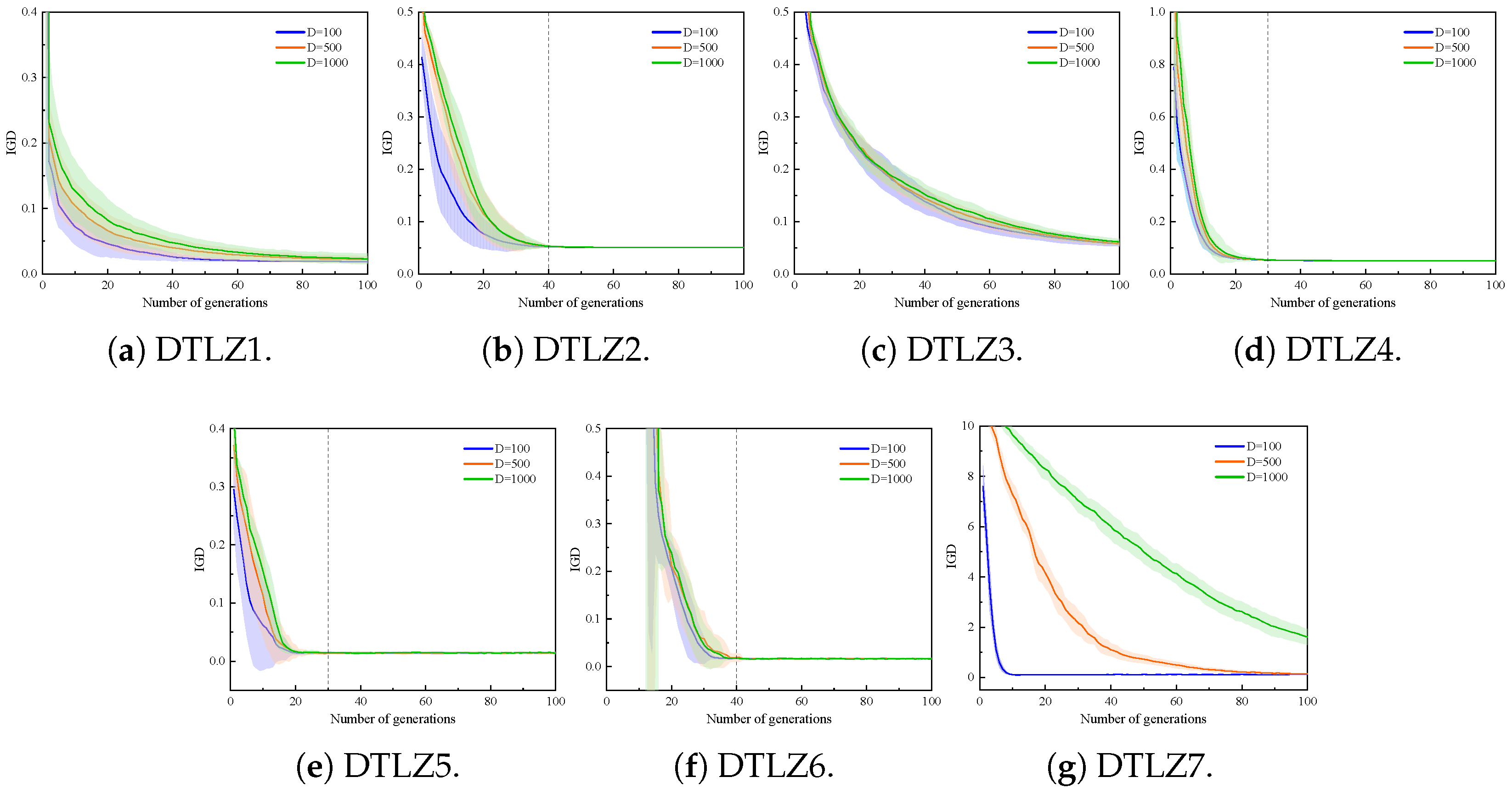
5.1.3. Performance of MOHA on Large-Scale MOPs with 1000 Decision Variables

As mentioned, MOHA demonstrates excellent performance on DTLZ problems with a number of decision variables of 30 and 50. In this section, we further challenge the ability of MOHA to solve MOPs on a larger scale of decision variables.

Figure 13 shows the average IGD metric convergence curve of MOHA on the DTLZ problems with dimensions from 100 to 1000. Overall, we can conclude that with the increase in decision variable dimensions, the convergence speed of the algorithm shows a decreasing trend, especially for DTLZ1, DTLZ3, and DTLZ7. Specifically, MOHA needs a higher number of iterations to solve the multimodal problems. This phenomenon occurs due to the fact that the landscape of the search domain can become exceedingly erratic as the number of dimensions increases. In contrast, the solution efficiency of MOHA remains high for the remaining test problems, which can converge within about 40 generations. In summary, MOHA is not sensitive to the dimensionality of decision variables, which is highly favorable for searching in high-dimensional decision spaces. For large-scale MOPs, MOHA is far more efficient than we can anticipate by balancing the exploitation and exploration capabilities. These tests illustrate the generality and efficiency of the proposed multi-objective local search operator. In the framework of gradient-based hybrid algorithms, the multi-objective local search operator is a powerful technique. It improves the ability of the algorithm to solve large-scale optimization problems. MOHA is less constrained by the dimensionality of the decision variables, and convergence can be achieved with a small number of evolutions. Therefore, this high efficiency is very meaningful for optimization problems with thousands of variables.

5.1.4. Efficiency Analysis of MOHA

From the previous analysis, the hybrid algorithm can fully leverage the advantages of both MOEA and MOGBA, achieving the goal of playing to their strengths and avoiding their weaknesses. Therefore, the algorithm can quickly approach the PF and improve the optimization efficiency dramatically. To verify the computational efficiency of MOHA,

Table 4. Approximate minimum number of iterations required for the algorithm to converge on the DTLZ problems.

Problem	M	D	MOHA	NSGA-III
DTLZ1	3	30	112	>1000
	3	50	130	>1000
	5	30	165	>1000
	5	50	188	>1000
DTLZ2	3	30	35	116
	3	50	40	158
	5	30	42	170
	5	50	48	293
DTLZ3	3	30	168	>1000
	3	50	195	>1000
	5	30	175	>1000
	5	50	210	>1000
DTLZ4	3	30	30	96
	3	50	35	184
	5	30	45	152
	5	50	48	283
DTLZ5	3	30	25	123
	3	50	30	195
	5	30	104	454
	5	50	115	611
DTLZ6	3	30	36	248
	3	50	55	692
	5	30	126	967
	5	50	144	>1000
DTLZ7	3	30	33	150
	3	50	35	216
	5	30	40	265
	5	50	48	352

summarizes the minimum number of iterations for MOHA and NSGA-III to reach convergence. From the table, since DTLZ1 and DTLZ3 are multimodal functions, the convergence speed of NSGA-III on such functions is very slow and requires greater than 1000 generations to find the Pareto optimal solutions. However, the MOHA can converge within about 210 generations, with an efficiency improvement of about five times. It is worth noting that there is a significant improvement of approximately 10 times when applying the mentioned approach on the 30-dimensional DTLZ1 problem. For the two sets of non-convex functions DTLZ2 and DTLZ4, NSGA-III can find the Pareto optimal solution within 300 generations, while MOHA requires only 50 generations. This illustrates that MOHA can solve non-convex problems effectively and converge six times faster than NSGA-III. Then, DTLZ5 and DTLZ6 are concave with degenerate PF functions, and the efficiency of MOHA is about seven times higher than that of NSGA-III. Finally, for DTLZ7, a concave/convex mixed, multimodal, discontinuous function, both MOHA and NSGA-III are able to find the Pareto optimal solution, but MOHA is still more efficient than NSGA-III.

To sum up, as the dimensionality of the objective and decision variables increases, the number of iterations of NSGA-III increases significantly, which not only increases the computational cost but may even lead to failure to search for the approximate PF. On all the DTLZ problems, the proposed MOHA always converges with a smaller number of iterations than NSGA-III. MOHA generates new offspring by mixing individuals carrying elite knowledge with MOEA through a local search of a small number of individuals. The result is a significant increase in efficiency, far exceeding our expectations. In addition, MOHA is less constrained by dimensionality, and the efficiency is generally improved by about 5–10 times with different dimensional DTLZ problems. Therefore, we can conclude that the offspring generation mechanism based on the MOGBA contributes to the rapid convergence of the algorithm and enhances the exploitation ability. By combining these two complementary offspring generation methods, the proposed MOHA is efficient and robust for various types of problems. MOHA has great potential for solving large-scale MOPs with high efficiency.

5.2. Performance Comparison between GS-MOHA and Existing SAEAs

A large population will occupy too many evaluations, which is not conducive to algorithm optimization, and the computational cost is high for excessively large evaluation times. Therefore, the initial population size is 100 and the maximum number of expensive fitness evaluations is set to 300. Both MOEA/D-EGO and K-RVEA have adopted Kriging as a surrogate model. The Kriging model is known to be unsuitable for high-dimensional problems due to the “dimension disaster”. Generally, the sampling point dimension of the Kriging model does not exceed 10 dimensions to ensure its accuracy and reliability. For expensive MOPs, when the dimensionality of the decision variables is greater than 10 ($D>10$), they can be called high-dimensional problems [29]. Therefore, we compared the performance of the three algorithms on DTLZ problems with decision variables dimensions of 10, 20, and 30. For a fair comparison, the remaining parameters of MOEA/D-EGO and K-RVEA are the same as in the literature [26,27], except for the modification of the population size. The algorithm terminates when the number of true fitness evaluations reaches 300. For each test problem, the algorithm was executed independently a total of 20 times. This section also uses IGD and HV to evaluate the performance of the algorithms.

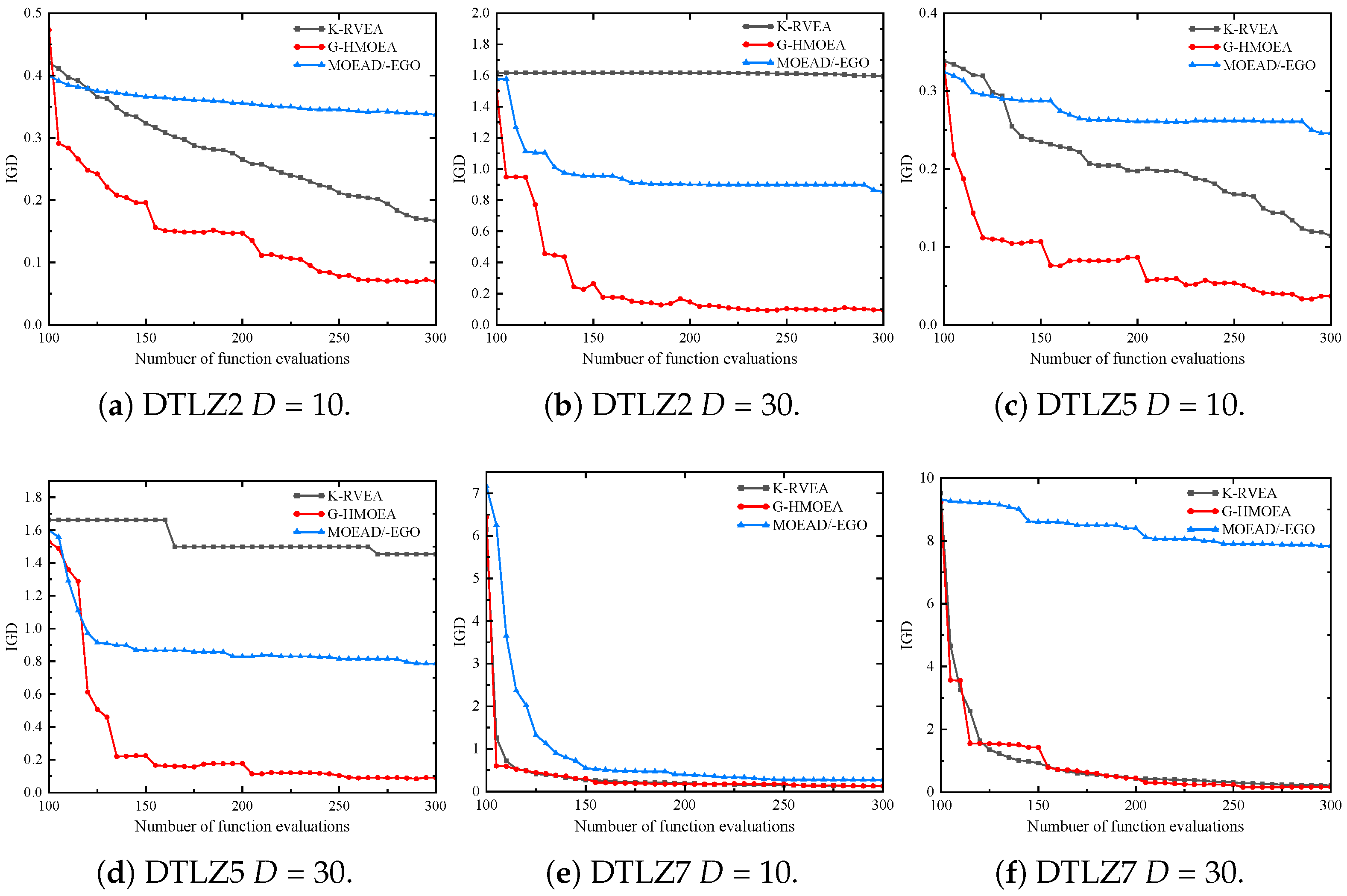
5.2.1. Experimental Results of Algorithms in Different Dimensions

Through

Table 5. IGD metric values of three algorithms on DTLZ problems, where the best result on each test problem is displayed in black and bold.

Problem	M	D	MOEA/D-EGO	K-RVEA	GS-MOHA
DTLZ1	3	10	$8.1113\times {10}^1(1.56\times {10}^1)-$	$8.9763\times {10}^1(2.03\times {10}^1)-$	$\mathbf{4}.\mathbf{4856}\times {\mathbf{10}}^{\mathbf{1}}(\mathbf{1}.\mathbf{48}\times {\mathbf{10}}^{\mathbf{1}})$
	3	20	$2.2247\times {10}^2(4.32\times {10}^1)-$	$3.2528\times {10}^2(4.39\times {10}^1)-$	$\mathbf{1}.\mathbf{0378}\times {\mathbf{10}}^{\mathbf{2}}(\mathbf{2}.\mathbf{47}\times {\mathbf{10}}^{\mathbf{1}})$
	3	30	$4.4293\times {10}^2(1.33\times {10}^2)-$	$5.9754\times {10}^2(4.73\times {10}^1)-$	$\mathbf{2}.\mathbf{6745}\times {\mathbf{10}}^{\mathbf{2}}(\mathbf{5}.\mathbf{59}\times {\mathbf{10}}^{\mathbf{1}})$
DTLZ2	3	10	$3.4606\times {10}^{-1}(2.19\times {10}^{-2})-$	$1.6513\times {10}^{-1}(3.07\times {10}^{-2})-$	$\mathbf{6}.\mathbf{3519}\times {\mathbf{10}}^{-\mathbf{2}}(\mathbf{2}.\mathbf{96}\times {\mathbf{10}}^{-\mathbf{2}})$
	3	20	$6.2647\times {10}^{-1}(7.29\times {10}^{-2})-$	$8.8597\times {10}^{-1}(1.06\times {10}^{-1})-$	$\mathbf{7}.\mathbf{1353}\times {\mathbf{10}}^{-\mathbf{2}}(\mathbf{4}.\mathbf{57}\times {\mathbf{10}}^{-\mathbf{2}})$
	3	30	$8.5044\times {10}^{-1}(1.24\times {10}^{-1})-$	$1.5940\times {10}^0(1.09\times {10}^{-1})-$	$\mathbf{9}.\mathbf{3448}\times {\mathbf{10}}^{-\mathbf{2}}(\mathbf{9}.\mathbf{13}\times {\mathbf{10}}^{-\mathbf{2}})$
DTLZ3	3	10	$1.8837\times {10}^2(1.95\times {10}^1)-$	$2.4005\times {10}^2(5.31\times {10}^1)-$	$\mathbf{1}.\mathbf{2479}\times {\mathbf{10}}^{\mathbf{2}}(\mathbf{2}.\mathbf{14}\times {\mathbf{10}}^{\mathbf{1}})$
	3	20	$5.2358\times {10}^2(9.68\times {10}^1)=$	$9.4022\times {10}^2(7.54\times {10}^1)-$	$\mathbf{4}.\mathbf{5657}\times {\mathbf{10}}^{\mathbf{2}}(\mathbf{7}.\mathbf{28}\times {\mathbf{10}}^{\mathbf{1}})$
	3	30	$9.4924\times {10}^2(2.28\times {10}^2)-$	$1.7254\times {10}^3(1.24\times {10}^2)-$	$\mathbf{6}.\mathbf{9858}\times {\mathbf{10}}^{\mathbf{2}}(\mathbf{8}.\mathbf{90}\times {\mathbf{10}}^{\mathbf{1}})$
DTLZ4	3	10	$6.2575\times {10}^{-1}(5.93\times {10}^{-2})-$	$4.0569\times {10}^{-1}(1.02\times {10}^{-1})=$	$\mathbf{3}.\mathbf{7943}\times {\mathbf{10}}^{-\mathbf{1}}(\mathbf{3}.\mathbf{97}\times {\mathbf{10}}^{-\mathbf{2}})$
	3	20	$1.1737\times {10}^0(1.17\times {10}^{-1})-$	$1.0677\times {10}^0(1.31\times {10}^{-1})-$	$\mathbf{5}.\mathbf{7216}\times {\mathbf{10}}^{-\mathbf{1}}(\mathbf{2}.\mathbf{44}\times {\mathbf{10}}^{-\mathbf{2}})$
	3	30	$1.4843\times {10}^0(2.26\times {10}^{-1})-$	$1.7804\times {10}^0(1.49\times {10}^{-1})-$	$\mathbf{7}.\mathbf{4431}\times {\mathbf{10}}^{-\mathbf{1}}(\mathbf{7}.\mathbf{37}\times {\mathbf{10}}^{-\mathbf{2}})$
DTLZ5	3	10	$2.4627\times {10}^{-1}(4.08\times {10}^{-2})-$	$1.1278\times {10}^{-1}(3.96\times {10}^{-2})-$	$\mathbf{3}.\mathbf{7622}\times {\mathbf{10}}^{-\mathbf{2}}(\mathbf{1}.\mathbf{89}\times {\mathbf{10}}^{-\mathbf{3}})$
	3	20	$5.5126\times {10}^{-1}(8.99\times {10}^{-2})-$	$7.9328\times {10}^{-1}(8.33\times {10}^{-2})-$	$\mathbf{4}.\mathbf{3125}\times {\mathbf{10}}^{-\mathbf{2}}(\mathbf{8}.\mathbf{17}\times {\mathbf{10}}^{-\mathbf{3}})$
	3	30	$7.8638\times {10}^{-1}(1.39\times {10}^{-1})-$	$1.4810\times {10}^0(1.25\times {10}^{-1})-$	$\mathbf{9}.\mathbf{0656}\times {\mathbf{10}}^{-\mathbf{2}}(\mathbf{1}.\mathbf{52}\times {\mathbf{10}}^{-\mathbf{2}})$
DTLZ6	3	10	$1.8794\times {10}^0(6.22\times {10}^{-1})-$	$3.0309\times {10}^0(3.90\times {10}^{-1})$−	$\mathbf{1}.\mathbf{4268}\times {\mathbf{10}}^{\mathbf{0}}(\mathbf{5}.\mathbf{62}\times {\mathbf{10}}^{-\mathbf{1}})$
	3	20	$\mathbf{6}.\mathbf{8555}\times {\mathbf{10}}^{\mathbf{0}}(\mathbf{1}.\mathbf{48}\times {\mathbf{10}}^{\mathbf{0}})+$	$1.0630\times {10}^1(6.86\times {10}^{-1})-$	$8.1262\times {10}^0(7.02\times {10}^{-1})$
	3	30	$\mathbf{1}.\mathbf{1799}\times {\mathbf{10}}^{\mathbf{1}}(\mathbf{1}.\mathbf{79}\times {\mathbf{10}}^{\mathbf{0}})+$	$1.9665\times {10}^1(9.64\times {10}^{-1})-$	$1.3062\times {10}^1(1.32\times {10}^0)$
DTLZ7	3	10	$2.7282\times {10}^{-1}(1.19\times {10}^{-1})-$	$\mathbf{1}.\mathbf{2710}\times {\mathbf{10}}^{-\mathbf{1}}(\mathbf{2}.\mathbf{15}\times {\mathbf{10}}^{-\mathbf{2}})+$	$1.3062\times {10}^{-1}(3.22\times {10}^{-2})$
	3	20	$4.7749\times {10}^0(1.23\times {10}^0)-$	$\mathbf{1}.\mathbf{6647}\times {\mathbf{10}}^{-\mathbf{1}}(\mathbf{2}.\mathbf{29}\times {\mathbf{10}}^{-\mathbf{2}})+$	$1.7846\times {10}^{-1}(2.47\times {10}^{-2})$
	3	30	$7.3196\times {10}^0(1.20\times {10}^0)-$	$2.3256\times {10}^{-1}(6.18\times {10}^{-2})=$	$\mathbf{1}.\mathbf{9245}\times {\mathbf{10}}^{-\mathbf{1}}(\mathbf{5}.\mathbf{74}\times {\mathbf{10}}^{-\mathbf{2}})$
+/−/=			2/18/1	2/17/2	N/A

and

Table 6. HV metric values of three algorithms on DTLZ problems, where the best result on each test problem is displayed in black and bold.

Problem	M	D	MOEA/D-EGO	KRVEA	GS-MOHA
DTLZ1	3	10	$0.0000\times {10}^0(0.00\times {10}^0)=$	$0.0000\times {10}^0(0.00\times {10}^0)=$	$0.0000\times {10}^0(0.00\times {10}^0)$
	3	20	$0.0000\times {10}^0(0.00\times {10}^0)=$	$0.0000\times {10}^0(0.00\times {10}^0)=$	$0.0000\times {10}^0(0.00\times {10}^0)$
	3	30	$0.0000\times {10}^0(0.00\times {10}^0)=$	$0.0000\times {10}^0(0.00\times {10}^0)=$	$0.0000\times {10}^0(0.00\times {10}^0)$
DTLZ2	3	10	$8.5641\times {10}^{-2}(2.70\times {10}^{-2})-$	$3.6223\times {10}^{-1}(6.05\times {10}^{-2})-$	$\mathbf{6}.\mathbf{4441}\times {\mathbf{10}}^{-\mathbf{1}}(\mathbf{5}.\mathbf{28}\times {\mathbf{10}}^{-\mathbf{2}})$
	3	20	$7.0733\times {10}^{-3}(1.17\times {10}^{-2})-$	$9.6527\times {10}^{-5}(4.32\times {10}^{-4})-$	$\mathbf{4}.\mathbf{2630}\times {\mathbf{10}}^{-\mathbf{1}}(\mathbf{3}.\mathbf{03}\times {\mathbf{10}}^{-\mathbf{2}})$
	3	30	$4.1283\times {10}^{-4}(1.85\times {10}^{-3})-$	$0.0000\times {10}^0(0.00\times {10}^0)-$	$\mathbf{2}.\mathbf{8064}\times {\mathbf{10}}^{-\mathbf{1}}(\mathbf{5}.\mathbf{70}\times {\mathbf{10}}^{-\mathbf{1}})$
DTLZ3	3	10	$0.0000\times {10}^0(0.00\times {10}^0)=$	$0.0000\times {10}^0(0.00\times {10}^0)=$	$0.0000\times {10}^0(0.00\times {10}^0)$
	3	20	$0.0000\times {10}^0(0.00\times {10}^0)=$	$0.0000\times {10}^0(0.00\times {10}^0)=$	$0.0000\times {10}^0(0.00\times {10}^0)$
	3	30	$0.0000\times {10}^0(0.00\times {10}^0)=$	$0.0000\times {10}^0(0.00\times {10}^0)=$	$0.0000\times {10}^0(0.00\times {10}^0)$
DTLZ4	3	10	$1.5058\times {10}^{-2}(2.19\times {10}^{-2})-$	$8.4914\times {10}^{-2}(1.01\times {10}^{-1})-$	$\mathbf{2}.\mathbf{7599}\times {\mathbf{10}}^{-\mathbf{1}}(\mathbf{1}.\mathbf{13}\times {\mathbf{10}}^{-\mathbf{1}})$
	3	20	$0.0000\times {10}^0(0.00\times {10}^0)-$	$0.0000\times {10}^0(0.00\times {10}^0)-$	$\mathbf{5}.\mathbf{9873}\times {\mathbf{10}}^{-\mathbf{2}}(\mathbf{2}.\mathbf{71}\times {\mathbf{10}}^{-\mathbf{2}})$
	3	30	$0.0000\times {10}^0(0.00\times {10}^0)-$	$0.0000\times {10}^0(0.00\times {10}^0)-$	$\mathbf{1}.\mathbf{4039}\times {\mathbf{10}}^{-\mathbf{2}}(\mathbf{2}.\mathbf{52}\times {\mathbf{10}}^{-\mathbf{2}})$
DTLZ5	3	10	$1.3048\times {10}^{-2}(1.31\times {10}^{-2})-$	$1.0287\times {10}^{-1}(3.24\times {10}^{-2})-$	$\mathbf{1}.\mathbf{9443}\times {\mathbf{10}}^{-\mathbf{1}}(\mathbf{1}.\mathbf{43}\times {\mathbf{10}}^{-\mathbf{3}})$
	3	20	$2.7393\times {10}^{-4}(1.23\times {10}^{-3})-$	$0.0000\times {10}^0(0.00\times {10}^0)-$	$\mathbf{1}.\mathbf{8305}\times {\mathbf{10}}^{-\mathbf{1}}(\mathbf{3}.\mathbf{28}\times {\mathbf{10}}^{-\mathbf{3}})$
	3	30	$0.0000\times {10}^0(0.00\times {10}^0)-$	$0.0000\times {10}^0(0.00\times {10}^0)-$	$\mathbf{6}.\mathbf{1012}\times {\mathbf{10}}^{-\mathbf{2}}(\mathbf{4}.\mathbf{81}\times {\mathbf{10}}^{-\mathbf{2}})$
DTLZ6	3	10	$\mathbf{4}.\mathbf{5578}\times {\mathbf{10}}^{-\mathbf{3}}(\mathbf{2}.\mathbf{04}\times {\mathbf{10}}^{-\mathbf{2}})=$	$0.0000\times {10}^0(0.00\times {10}^0)=$	$0.0000\times {10}^0(0.00\times {10}^0)$
	3	20	$0.0000\times {10}^0(0.00\times {10}^0)=$	$0.0000\times {10}^0(0.00\times {10}^0)=$	$0.0000\times {10}^0(0.00\times {10}^0)$
	3	30	$0.0000\times {10}^0(0.00\times {10}^0)=$	$0.0000\times {10}^0(0.00\times {10}^0)=$	$0.0000\times {10}^0(0.00\times {10}^0)$
DTLZ7	3	10	$1.8909\times {10}^{-1}(2.35\times {10}^{-2})-$	$\mathbf{2}.\mathbf{5303}\times {\mathbf{10}}^{-\mathbf{1}}(\mathbf{4}.\mathbf{39}\times {\mathbf{10}}^{-\mathbf{3}})+$	$2.2037\times {10}^{-1}(3.31\times {10}^{-2})$
	3	20	$0.0000\times {10}^0(0.00\times {10}^0)-$	$2.2474\times {10}^{-1}(6.93\times {10}^{-3})=$	$\mathbf{2}.\mathbf{5072}\times {\mathbf{10}}^{-\mathbf{1}}(\mathbf{2}.\mathbf{35}\times {\mathbf{10}}^{-\mathbf{2}})$
	3	30	$0.0000\times {10}^0(0.00\times {10}^0)-$	$1.9609\times {10}^{-1}(2.24\times {10}^{-2})-$	$\mathbf{2}.\mathbf{8748}\times {\mathbf{10}}^{-\mathbf{1}}(\mathbf{6}.\mathbf{52}\times {\mathbf{10}}^{-\mathbf{2}})$
+/−/=			0/12/9	1/10/10	N/A

, GS-MOHA achieves the best mean for 17 questions of the IGD metric and the best mean for 11 questions on the HV metric. For DTLZ1, DTLZ3, and DTLZ6, none of the algorithms can obtain a good Pareto distribution, which may require a higher number of evaluations. For other test problems, GS-MOHA outperforms the comparison algorithm in most situations. In addition, MOEA/D-EGO and K-RVEA performance decreases significantly when increasing from 10 to 30 dimensions, while GS-MOHA decreases slightly. This is made possible by the fact that both the GEKPLS model and the proposed MOHA are effective at solving high-dimensional decision variable problems. The combination of the two enables G-HOMEA the ability to solve expensive MOPs for high-dimensional decision variables. GS-MOHA inherits the advantages of the hybrid algorithm well and can obtain a satisfactory global optimal solution with a limited number of real fitness evaluations.

For further observations, the iteration curves of the mean IGD values of the three algorithms when the decision variables are 10 and 30 dimensions are plotted in Figure 14. Through comparison, the following three observations can be made. First, the IGD value of GS-MOHA decreases faster on all test functions and therefore converges more efficiently. It can be concluded that GS-MOHA is insensitive to changes in the dimensionality of decision variables. Second, as the dimension of decision variables increases, the convergence speed of MOEA/D-EGO and K-RVEA decreases significantly. For example, in the 30-dimensional DTLZ2 and DTLZ5 problems, the phenomenon of falling into the local optimum and thus failing to find the global optimum solution occurs. Although GS-MOHA also appears to be trapped in a local optimum, the algorithm could jump out of the local optimum and show excellent performance due to the superiority of the hybrid framework. Finally, the algorithm adopts the dual acceleration mechanism of the hybrid framework based on local search and the GEKPLS model based on gradient-enhanced Kriging, thus alleviating the “dimension disaster”.

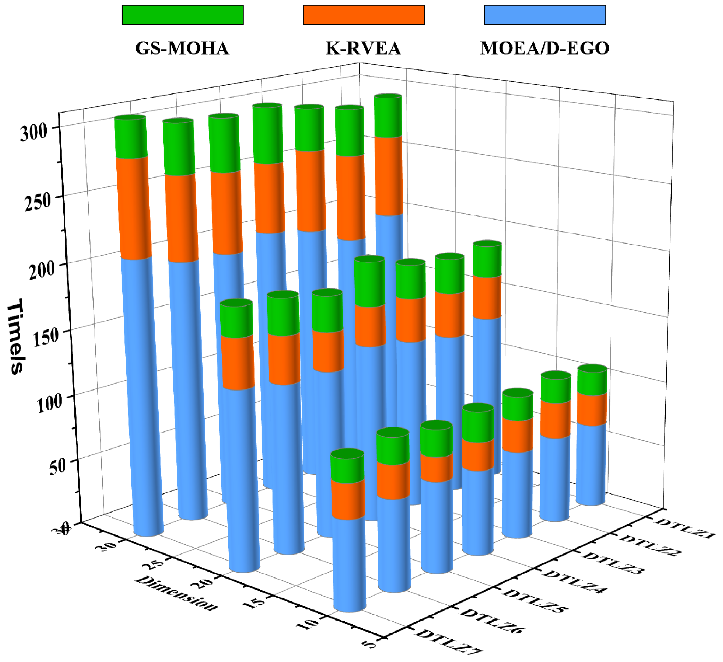
5.2.2. Efficiency Analysis of GS-MOHA

For the surrogate-assisted optimization algorithm, the time consumption is mainly generated by training the surrogate model and real fitness evaluation. With the same number of sampling points, the fitting accuracy and training time of the surrogate model deteriorates rapidly as the dimension of the decision variable increases. Therefore, the time consumption of the algorithm is one of the important metrics to measure its performance.

Figure 15 shows the mean running times of these three algorithms for different decision variable dimensions. According to the results in Figure 15, the overall running time of the algorithm tends to increase with the growth of dimensionality. Specifically, the runtime of GS-MOHA in the 10-dimensional DTLZ instances is significantly smaller than that of MOEA/D-EGO but similar to that of K-RVEA. For the 30-dimensional test problems, the computational efficiency of the proposed GS-MOHA is about two times that of K-RVEA and about five times higher than that of MOEA/D-EGO, which is demonstrated in Figure 15 clearly. The reason why the proposed GS-MOHA has high operating efficiency is because it adopts the GEKPLS surrogate model. The GEKPLS model has the advantage of fast training speed and high accuracy in high-dimensional space. In contrast, MOEA/D-EGO and K-RVEA use traditional Kriging models, so the training time increases significantly as the dimensionality of the decision variables increases. Furthermore, GS-MOHA adopts a hybrid algorithm framework, which also has a certain acceleration effect on the evolution of the algorithm. Based on the above empirical results, GS-MOHA can significantly reduce the optimization time required to solve expensive MOPs with high-dimensional decision variables and has good prospects for engineering applications.

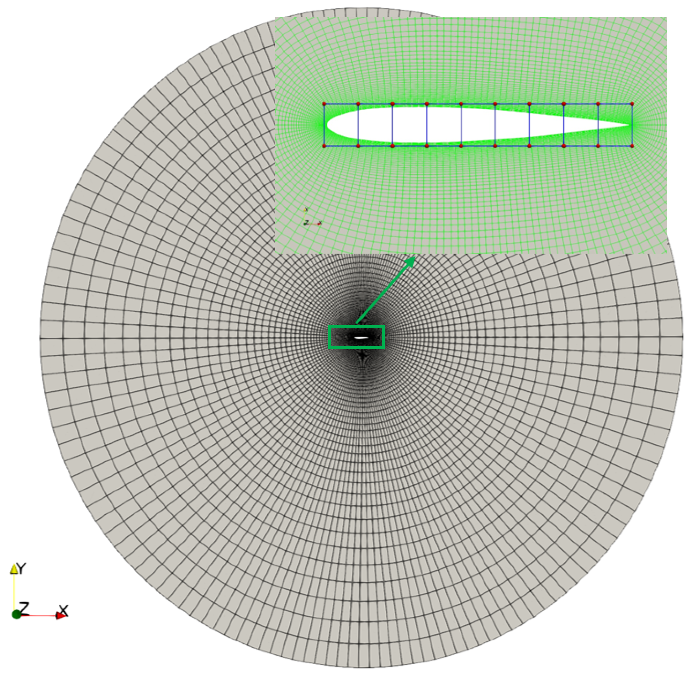
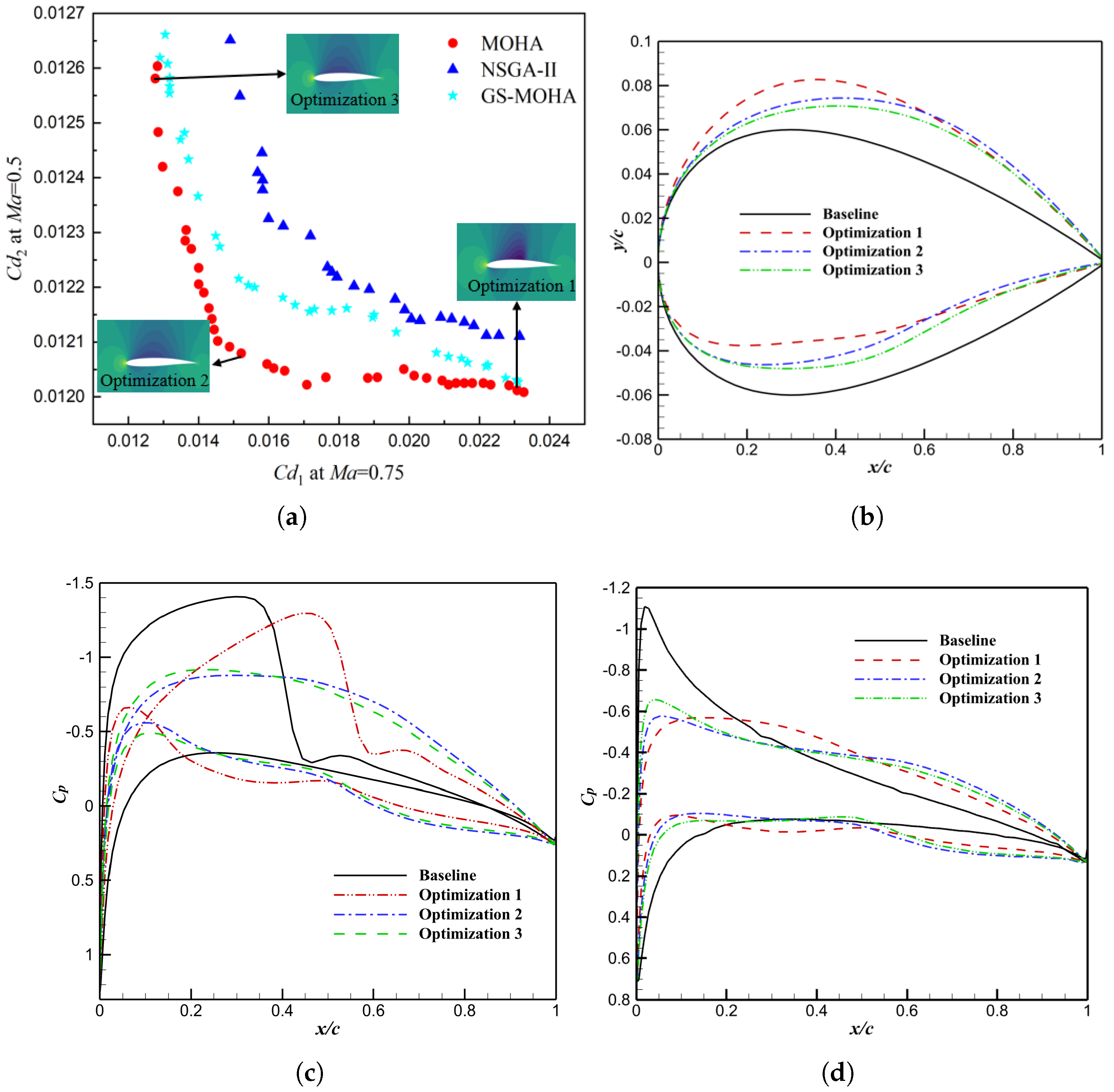
6. Multi-Objective Aerodynamic Shape Optimization of Airfoil

The airfoil shape design optimization problem [2,56] has been extensively studied to verify the efficiency of hybrid algorithms in aerodynamic optimization problems. Aircraft aerodynamic design experience has shown that the mechanism of increasing lift and decreasing drag is different in different speed domains, and thus the requirements for airfoil shape are significantly different. For the sake of simplicity, a bi-objective airfoil design optimization problem is used to verify the efficiency of the proposed algorithm and its value in engineering applications, considering two different flight states. A multi-objective optimization problem is carried out using the NACA0012 airfoil as the baseline airfoil. The objective of the optimization problem is to minimize the drag coefficient ($C_d$) in two states simultaneously by changing the airfoil shape of NACA0012. The initial design state is:

$$\begin{array}{cc}\hfill & \left(1\right)M{a}_1=0.75,R{e}_1=5.5\times {10}^6,{\alpha }_1={2.0}^{\circ }\hfill \\ \hfill & \left(2\right)M{a}_2=0.5,R{e}_2=4.5\times {10}^6,{\alpha }_2={2.5}^{\circ }\hfill \end{array}$$

(8)

where $M{a}_1$ and $M{a}_2$ represent Mach numbers, $R{e}_1$ and $R{e}_2$ are the Reynolds numbers, and ${\alpha }_1$ and ${\alpha }_2$ are the angles of attack. The computation of $C_d$ and lift coefficient ($C_l$) involves aerodynamic simulation, so the open-source DAFoam [57] solver was used. The solver uses the $S-A$ turbulence model to accurately simulate the airflow around the aircraft by solving the RANS equations. Furthermore, it has developed an efficient discrete adjoint method. With this solver, we can easily calculate the $C_d$, $C_l$ and gradient information of the airfoil. In addition, a structural meshing of the airfoil was performed with a mesh number of $4.6\times {10}^4$ and a first layer mesh height of $2\times {10}^{-5}$. The control points were then moved by the free-form deformation (FFD) [58] parameterization method, thus changing the shape of the airfoil of NACA0012. We used 22 design variables, which include the variations in FFD control points in the y-direction $(y_1,y_2,\cdots ,y_{20})$ and two angles of attack $({\alpha }_1,{\alpha }_2)$. A schematic diagram of the mesh and parameterization of the geometric model is shown in Figure 16.

The mathematical model of this multi-objective optimization problem is formulated as follows:

$$\left\{\begin{array}{c}\min :f_1\left(x\right)=C_{d1},f_2\left(x\right)=C_{d2}\hfill \\ s.t.:\begin{array}{cc}& A\ge A_0,t\ge 0.95t_0,C{l}_1\ge C{l}_{\mathrm{ini}1}\end{array},C{l}_2\ge C{l}_{\mathrm{ini}2}\hfill \end{array}\right.$$

(9)

where $A_0,t_0,C{l}_{\mathrm{ini}1}$, and $C{l}_{\mathrm{ini}2}$ are the area, thickness, and lift coefficients of the baseline airfoil for both states. Using the above optimization model, three algorithms NSGA-II, MOHA, and GS-MOHA are used for optimization comparison. The parameter settings and optimization results of the three algorithms are compared, as shown in

Table 7. Comparison of parameter settings and optimization efficiency of algorithms.

	NSGA-II	MOHA	GS-MOHA
Population size	50	50	50
Number of design variables	22	22	22
Number of CFD evaluations	4000	2000	1000
Number of gradient evaluations	-	115	1000
Number of CPU	16	16	16
Number of non-dominated solutions	25	37	33
CPU cost (h)	≈133	≈71	≈26

and Figure 17.

Optimization 1 has the best subsonic performance, and Optimization 3 is the best airfoil for transonic performance. By comparing the pressure distributions, it is observed that the shock waves in Optimization 2 and Optimization 3 are largely eliminated in the transonic state. Compared to the baseline airfoil, the optimized airfoil exhibits a maximum thickness shift towards the trailing edge, the increased camber, and a concave shape on the lower surface. These changes help improve the lift characteristics and reduce the drag of the airfoil in both subsonic and transonic states.

Compared with NSGA-II, MOHA exhibits significantly superior PF distribution and convergence with only 2000 evaluations. Therefore, this validates the superiority of the proposed algorithm as the introduction of gradient information in evolutionary algorithms can enhance optimization results and improve efficiency. Moreover, the optimization results of GS-MOHA are also superior to those of NSGA-II while consuming only a quarter of the computational iterations for flow field calculations. Hence, this signifies that under limited flow field calculation iterations, the surrogate-assisted algorithm can significantly reduce the optimization time and demonstrate tremendous engineering practical value.

Although the example of airfoil optimization is relatively simple, it still effectively demonstrates the superiority of the proposed algorithms. When faced with the optimization of complex shapes, the decision variables increase, leading to an increase in the number of iterations of the algorithm and the population size. But the essence of the optimization algorithms remains the same. It is crucial to consider parameterization, flow field solving, and adjoint solving, among other issues. Therefore, the proposed algorithm has the potential to be fully extended to solve complex aerodynamic shape optimization problems.

7. Conclusions

This paper proposed two efficient optimization algorithms (i.e., MOHA and GS-MOHA) based on a bilayer parallel hybrid algorithm framework to solve large-scale MOPs and expensive MOPs in engineering optimization. The hybrid framework couples global evolutionary and local multi-objective gradient search techniques, which jointly determine the performance of the algorithm. Then, the diversity and convergence of the algorithm are balanced through the information exchange of the bilayer space. A multi-objective gradient operator based on dynamic random weights is designed to improve the ability of GBAs to find non-convex and disconnected PFs in MOHA. The efficiency of the algorithm can be greatly improved by incorporating individuals with excellent genes after gradient update into the evolutionary process. Moreover, embedding the GEKPLS surrogate model in the hybrid algorithm framework further improves the engineering application capability of MOHA. Eventually, in order to validate the performance of the proposed algorithm, the DTLZ problem with different numbers of decision variables and objectives as well as the multi-objective shape optimization problem of NACA0012 are tested. The following conclusions can be achieved:

(1)

The proposed MOHA is insensitive to the dimension of MOPs. For benchmark test functions with different numbers of decision variables (30, 50) and objectives (3, 5), the convergence and diversity of MOHA are significantly better than the comparison algorithms (i.e., MOEA/D, NSGA-III, RVEA, and VaEA) and the computational efficiency is increased by about 5–10 times. Furthermore, MOHA still illustrates good stability and efficiency for large-scale MOPs with decision variables up to 1000 dimensions. This demonstrates that MOHA is an efficient optimization algorithm capable of solving large-scale MOPs.

(2)

GS-MOHA could solve expensive MOPs efficiently in high dimensions ($D>10$). GEKPLS utilizes the PLS method to accelerate Kriging construction. The higher the dimensionality of the decision variables, the more significant the efficiency improvement of the algorithm. For the 30-dimensional DTLZ problems, the runtime of GS-MOHA is about half that of K-RVEA and one-fifth that of MOEA/D-EGO.

(3)

The rational use of low-cost gradient information is a very promising approach in the framework of hybrid algorithms. We can not only promote the evolution of MOEA and maintain population diversity through multi-objective gradient search but also use this low-cost gradient information to improve the accuracy of Kriging.

(4)

Computing gradients in local search can use the adjoint method, which does not impose an additional huge computational burden, because the cost of computing gradients using the adjoint method is roughly equivalent to that of fitness evaluation. Moreover, unlike the finite-difference approximation, the computational cost of the adjoint method is independent of the dimensionality of the decision variables. This makes it easy to apply our proposed two hybrid algorithms to the high-dimensional aerodynamic shape optimization design.

(5)

In this work, the optimization efficiency of MOHA and GS-MOHA was preliminarily validated on a multi-objective optimization problem of NACA0012 with 22 design variables. The results demonstrated promising engineering application potential. The proposed algorithms will be applied to the multi-objective aerodynamic optimization of complex aircraft shapes in the future.

References

1. Tang, Z.; Zhang, L. A new Nash optimization method based on alternate elitist information exchange for multi-objective aerodynamic shape design. Appl. Math. Model. 2019, 68, 244–266. [Google Scholar] [CrossRef]
2. Jing, S.; Zhao, Q.; Zhao, G.; Wang, Q. Multi-Objective Airfoil Optimization Under Unsteady-Freestream Dynamic Stall Conditions. J. Aircr. 2023, 60, 293–309. [Google Scholar] [CrossRef]
3. Anosri, S.; Panagant, N.; Champasak, P.; Bureerat, S.; Thipyopas, C.; Kumar, S.; Pholdee, N.; Yıldız, B.S.; Yildiz, A.R. A Comparative Study of State-of-the-art Metaheuristics for Solving Many-objective Optimization Problems of Fixed Wing Unmanned Aerial Vehicle Conceptual Design. Arch. Comput. Methods Eng. 2023, 30, 3657–3671. [Google Scholar] [CrossRef]
4. Yu, Y.; Lyu, Z.; Xu, Z.; Martins, J.R. On the influence of optimization algorithm and initial design on wing aerodynamic shape optimization. Aerosp. Sci. Technol. 2018, 75, 183–199. [Google Scholar] [CrossRef]
5. Dai, Y.H. Convergence properties of the BFGS algoritm. Siam J. Optim. 2002, 13, 693–701. [Google Scholar] [CrossRef]
6. Zhu, C.; Byrd, R.H.; Lu, P.; Nocedal, J. Algorithm 778: L-BFGS-B: Fortran subroutines for large-scale bound-constrained optimization. ACM Trans. Math. Softw. (TOMS) 1997, 23, 550–560. [Google Scholar] [CrossRef]
7. Yuan, G.; Hu, W. A conjugate gradient algorithm for large-scale unconstrained optimization problems and nonlinear equations. J. Inequal. Appl. 2018, 2018, 1–19. [Google Scholar] [CrossRef]
8. Bomze, I.M.; Demyanov, V.F.; Fletcher, R.; Terlaky, T.; Fletcher, R. Nonlinear Optimization; Springer: Berlin, Germany, 2010. [Google Scholar]
9. Jameson, A. Optimum aerodynamic design using CFD and control theory. In Proceedings of the 12th Computational Fluid Dynamics Conference, San Diego, CA, USA, 19–22 June 1995; p. 1729. [Google Scholar]
10. Wang, Z.; Pei, Y.; Li, J. A Survey on Search Strategy of Evolutionary Multi-Objective Optimization Algorithms. Appl. Sci. 2023, 13, 4643. [Google Scholar] [CrossRef]
11. Lyu, Z.; Martins, J.R. Aerodynamic design optimization studies of a blended-wing-body aircraft. J. Aircr. 2014, 51, 1604–1617. [Google Scholar] [CrossRef]
12. Lyu, Z.; Kenway, G.K.; Martins, J.R. Aerodynamic shape optimization investigations of the common research model wing benchmark. AIAA J. 2015, 53, 968–985. [Google Scholar] [CrossRef]
13. Gao, W.; Wang, Y.; Liu, L.; Huang, L. A gradient-based search method for multi-objective optimization problems. Inf. Sci. 2021, 578, 129–146. [Google Scholar] [CrossRef]
14. Zhao, X.; Tang, Z.; Cao, F.; Zhu, C.; Periaux, J. An Efficient Hybrid Evolutionary Optimization Method Coupling Cultural Algorithm with Genetic Algorithms and Its Application to Aerodynamic Shape Design. Appl. Sci. 2022, 12, 3482. [Google Scholar] [CrossRef]
15. Kiani, F.; Nematzadeh, S.; Anka, F.A.; Findikli, M.A. Chaotic Sand Cat Swarm Optimization. Mathematics 2023, 11, 2340. [Google Scholar] [CrossRef]
16. He, C.; Zhang, Y.; Gong, D.; Ji, X. A review of surrogate-assisted evolutionary algorithms for expensive optimization problems. Expert Syst. Appl. 2023, 217, 119495. [Google Scholar] [CrossRef]
17. Li, J.; Cai, J.; Qu, K. Surrogate-based aerodynamic shape optimization with the active subspace method. Struct. Multidiscip. Optim. 2019, 59, 403–419. [Google Scholar] [CrossRef]
18. He, Y.; Sun, J.; Song, P.; Wang, X.; Usmani, A.S. Preference-driven Kriging-based multiobjective optimization method with a novel multipoint infill criterion and application to airfoil shape design. Aerosp. Sci. Technol. 2020, 96, 105555. [Google Scholar] [CrossRef]
19. Yang, Z.; Qiu, H.; Gao, L.; Chen, L.; Liu, J. Surrogate-assisted MOEA/D for expensive constrained multi-objective optimization. Inf. Sci. 2023, 639, 119016. [Google Scholar] [CrossRef]
20. Khuri, A.I.; Mukhopadhyay, S. Response surface methodology. Wiley Interdiscip. Rev. Comput. Stat. 2010, 2, 128–149. [Google Scholar] [CrossRef]
21. Martin, J.D.; Simpson, T.W. Use of Kriging models to approximate deterministic computer models. AIAA J. 2005, 43, 853–863. [Google Scholar] [CrossRef]
22. Dongare, A.; Kharde, R.; Kachare, A.D. Introduction to artificial neural network. Int. J. Eng. Innov. Technol. (IJEIT) 2012, 2, 189–194. [Google Scholar]
23. Buhmann, M.D. Radial basis functions. Acta Numer. 2000, 9, 1–38. [Google Scholar] [CrossRef]
24. Zhong, L.; Liu, R.; Miao, X.; Chen, Y.; Li, S.; Ji, H. Compressor Performance Prediction Based on the Interpolation Method and Support Vector Machine. Aerospace 2023, 10, 558. [Google Scholar] [CrossRef]
25. Knowles, J. ParEGO: A hybrid algorithm with on-line landscape approximation for expensive multiobjective optimization problems. IEEE Trans. Evol. Comput. 2006, 10, 50–66. [Google Scholar] [CrossRef]
26. Zhang, Q.; Liu, W.; Tsang, E.; Virginas, B. Expensive multiobjective optimization by MOEA/D with Gaussian process model. IEEE Trans. Evol. Comput. 2009, 14, 456–474. [Google Scholar] [CrossRef]
27. Chugh, T.; Jin, Y.; Miettinen, K.; Hakanen, J.; Sindhya, K. A surrogate-assisted reference vector guided evolutionary algorithm for computationally expensive many-objective optimization. IEEE Trans. Evol. Comput. 2016, 22, 129–142. [Google Scholar] [CrossRef]
28. Cai, X.; Ruan, G.; Yuan, B.; Gao, L. Complementary surrogate-assisted differential evolution algorithm for expensive multi-objective problems under a limited computational budget. Inf. Sci. 2023, 632, 791–814. [Google Scholar] [CrossRef]
29. Bouhlel, M.A.; Martins, J.R.R.A. Gradient-enhanced Kriging for high-dimensional problems. Eng. Comput. 2019, 35, 157–173. [Google Scholar] [CrossRef]
30. Hong, W.J.; Yang, P.; Tang, K. Evolutionary Computation for Large-scale Multi-objective Optimization: A Decade of Progresses. Int. J. Autom. Comput. 2021, 18, 155–169. [Google Scholar] [CrossRef]
31. Xu, Y.; Zhang, H.; Huang, L.; Qu, R.; Nojima, Y. A Pareto Front grid guided multi-objective evolutionary algorithm. Appl. Soft Comput. 2023, 136, 110095. [Google Scholar] [CrossRef]
32. Cao, B.; Zhao, J.; Gu, Y.; Ling, Y.; Ma, X. Applying graph-based differential grouping for multiobjective large-scale optimization. Swarm Evol. Comput. 2020, 53, 100626. [Google Scholar] [CrossRef]
33. Huband, S.; Hingston, P.; Barone, L.; While, L. A review of multiobjective test problems and a scalable test problem toolkit. IEEE Trans. Evol. Comput. 2006, 10, 477–506. [Google Scholar] [CrossRef]
34. Deb, K.; Pratap, A.; Agarwal, S.; Meyarivan, T. A fast and elitist multiobjective genetic algorithm: NSGA-II. IEEE Trans. Evol. Comput. 2002, 6, 182–197. [Google Scholar] [CrossRef]
35. Marler, R.T.; Arora, J.S. The weighted sum method for multi-objective optimization: New insights. Struct. Multidiscip. Optim. 2010, 41, 853–862. [Google Scholar] [CrossRef]
36. Deb, K.; Jain, H. An Evolutionary Many-Objective Optimization Algorithm Using Reference-Point-Based Nondominated Sorting Approach, Part I: Solving Problems With Box Constraints. IEEE Trans. Evol. Comput. 2014, 18, 577–601. [Google Scholar] [CrossRef]
37. Zitzler, E.; Thiele, L.; Laumanns, M.; Fonseca, C.M.; Da Fonseca, V.G. Performance assessment of multiobjective optimizers: An analysis and review. IEEE Trans. Evol. Comput. 2003, 7, 117–132. [Google Scholar] [CrossRef]
38. Zuhal, L.R.; Zakaria, K.; Palar, P.S.; Shimoyama, K.; Liem, R.P. Polynomial-chaos–Kriging with gradient information for surrogate modeling in aerodynamic design. AIAA J. 2021, 59, 2950–2967. [Google Scholar] [CrossRef]
39. Han, Z.H.; Zhang, Y.; Song, C.X.; Zhang, K.S. Weighted gradient-enhanced Kriging for high-dimensional surrogate modeling and design optimization. Aiaa J. 2017, 55, 4330–4346. [Google Scholar] [CrossRef]
40. Liu, F.; Zhang, Q.; Han, Z. MOEA/D with gradient-enhanced Kriging for expensive multiobjective optimization. Nat. Comput. 2022, 22, 329–339. [Google Scholar] [CrossRef]
41. Bouhlel, M.A.; Bartoli, N.; Otsmane, A.; Morlier, J. Improving Kriging surrogates of high-dimensional design models by Partial Least Squares dimension reduction. Struct. Multidiscip. Optim. 2016, 53, 935–952. [Google Scholar] [CrossRef]
42. Tang, Z.; Hu, X.; Périaux, J. Multi-level Hybridized Optimization Methods Coupling Local Search Deterministic and Global Search Evolutionary Algorithms. Arch. Comput. Methods Eng. 2020, 27, 939–975. [Google Scholar] [CrossRef]
43. Zhang, Y.; Wang, G.; Wang, H. NSGA-II/SDR-OLS: A Novel Large-Scale Many-Objective Optimization Method Using Opposition-Based Learning and Local Search. Mathematics 2023, 11, 1911. [Google Scholar] [CrossRef]
44. Bouaziz, H.; Bardou, D.; Berghida, M.; Chouali, S.; Lemouari, A. A novel hybrid multi-objective algorithm to solve the generalized cubic cell formation problem. Comput. Oper. Res. 2023, 150, 106069. [Google Scholar] [CrossRef]
45. Nayyef, H.M.; Ibrahim, A.A.; Mohd Zainuri, M.A.A.; Zulkifley, M.A.; Shareef, H. A Novel Hybrid Algorithm Based on Jellyfish Search and Particle Swarm Optimization. Mathematics 2023, 11, 3210. [Google Scholar] [CrossRef]
46. Cao, B.; Zhang, W.; Wang, X.; Zhao, J.; Gu, Y.; Zhang, Y. A memetic algorithm based on two_Arch2 for multi-depot heterogeneous-vehicle capacitated arc routing problem. Swarm Evol. Comput. 2021, 63, 100864. [Google Scholar] [CrossRef]
47. Deb, K.; Goel, T. A Hybrid Multi-objective Evolutionary Approach to Engineering Shape Design. In Proceedings of the Evolutionary Multi-Criterion Optimization, Zurich, Switzerland, 7–9 March 2001; Springer: Berlin/Heidelberg, Germany, 2001; pp. 385–399. [Google Scholar]
48. Sun, Y.; Zhang, L.; Gu, X. A hybrid co-evolutionary cultural algorithm based on particle swarm optimization for solving global optimization problems. Neurocomputing 2012, 98, 76–89. [Google Scholar] [CrossRef]
49. Forrester, A.I.J.; Keane, A.J. Recent advances in surrogate-based optimization. Prog. Aerosp. Sci. 2009, 45, 50–79. [Google Scholar] [CrossRef]
50. Parr, J.M.; Keane, A.J.; Forrester, A.I.; Holden, C.M. Infill sampling criteria for surrogate-based optimization with constraint handling. Eng. Optim. 2012, 44, 1147–1166. [Google Scholar] [CrossRef]
51. Han, Z.H. SurroOpt: A generic surrogate-based optimization code for aerodynamic and multidisciplinary design. In Proceedings of the 30th Congress of the International Council of the Aeronautical Sciences—ICAS 2016, Daejeon, Republic of Korea, 25–30 September 2016. [Google Scholar]
52. Zhang, Q.; Li, H. MOEA/D: A Multiobjective Evolutionary Algorithm Based on Decomposition. IEEE Trans. Evol. Comput. 2007, 11, 712–731. [Google Scholar] [CrossRef]
53. Cheng, R.; Jin, Y.; Olhofer, M.; Sendhoff, B. A Reference Vector Guided Evolutionary Algorithm for Many-Objective Optimization. IEEE Trans. Evol. Comput. 2016, 20, 773–791. [Google Scholar] [CrossRef]
54. Xiang, Y.; Zhou, Y.; Li, M.; Chen, Z. A Vector Angle-Based Evolutionary Algorithm for Unconstrained Many-Objective Optimization. IEEE Trans. Evol. Comput. 2017, 21, 131–152. [Google Scholar] [CrossRef]
55. Zhang, X.; Tian, Y.; Cheng, R.; Jin, Y. A Decision Variable Clustering-Based Evolutionary Algorithm for Large-Scale Many-Objective Optimization. IEEE Trans. Evol. Comput. 2018, 22, 97–112. [Google Scholar] [CrossRef]
56. Areias, P.; Correia, R.; Melicio, R. Airfoil Analysis and Optimization Using a Petrov–Galerkin Finite Element and Machine Learning. Aerospace 2023, 10, 638. [Google Scholar] [CrossRef]
57. He, P.; Mader, C.A.; Martins, J.R.; Maki, K.J. Dafoam: An open-source adjoint framework for multidisciplinary design optimization with openfoam. AIAA J. 2020, 58, 1304–1319. [Google Scholar] [CrossRef]
58. Kenway, G.; Kennedy, G.; Martins, J.R. A CAD-free approach to high-fidelity aerostructural optimization. In Proceedings of the 13th AIAA/ISSMO Multidisciplinary Analysis Optimization Conference, Ft. Worth, TX, USA, 13–15 September 2010; p. 9231. [Google Scholar]
Figure 1. The proportion of non-dominated solutions in relation to (a) the number of objectives and (b) the dimension of decision variables, respectively. The error bar is a standard deviation.
Mathematics 11 03844 g001
Figure 2. Weighted sum method applied to MOP with non-convex Pareto front. A and B are extreme points and C is the local optimum point.
Mathematics 11 03844 g002
Figure 3. Comparison of average IGD convergence curve of MOGBA and NSGA-III algorithm on (a) DTLZ2 D = 10 and (b) DTLZ2 D = 30. The error band is the standard deviation.
Mathematics 11 03844 g003
Figure 4. Performance comparison of surrogate models: (a) accuracy at different number of sampling points when d = 10 , (b) accuracy at different number of sampling points when d = 20 , (c) training time with different number of sampling points, and (d) training time of GEKPLS in different dimensions.
Mathematics 11 03844 g004
Figure 5. High-dimensional global optimization problems faced in aerodynamic shape design.
Mathematics 11 03844 g005
Figure 6. The process of proposing the algorithm in this paper.
Mathematics 11 03844 g006
Figure 7. Improving the quality of MOEA solution sets using local search techniques.
Mathematics 11 03844 g007
Figure 8. Hybrid algorithm framework of global evolution and multi-objective local gradient search.
Mathematics 11 03844 g008
Figure 9. Influence of local search frequency P on algorithm performance: (a) Box plot of the MOHA for different P (red dots are outliers, black dots are means, and black dashed lines are medians), and (b) average IGD convergence curves for different P.
Mathematics 11 03844 g009
Figure 10. The evolution of PF for different algorithms on ZDT2: (a) the evolution process of PF after 100 generations with NSGA-III, and (b,c) the evolution process of PF after 20 generations with MOGBA and MOHA. The red dots are the offspring generated by the local search.
Mathematics 11 03844 g010
Figure 11. Flow chart of the GS-MOHA algorithm.
Mathematics 11 03844 g011
Figure 12. Effect of model update frequency K on algorithm performance: (a) box plot of different frequencies on DTLZ2 and (b) box plot of different frequencies on DTLZ7. (Red dots are outliers, black dots are means, and black dashed lines are medians.)
Mathematics 11 03844 g012
Figure 13. Average IGD convergence curves of MOHA on 100, 500, and 1000-dimensional DTLZ problems, averaged over 20 runs. The error band is the standard deviation.
Mathematics 11 03844 g013
Figure 14. Convergence curves of three algorithms in the 10- and 30-dimensional DTLZ2, DTLZ5, and DTLZ7 problems.
Mathematics 11 03844 g014
Figure 15. 3D stacked bar chart of algorithm runtimes.
Mathematics 11 03844 g015
Figure 16. Mesh and FFD control points of the NACA0012.
Mathematics 11 03844 g016
Figure 17. Comparison of airfoil optimization results. (a) Comparison of the PFs of the three algorithms; (b) comparison of the geometrical shapes of the airfoil; (c) comparison of the pressure coefficient distribution of airfoil in State 1; and (d) comparison of the pressure coefficient distribution of airfoil in State 2.
Mathematics 11 03844 g017