1. Introduction
Elastic modulus (
E) is one of the key parameters characterizing the properties of rock, and the accurate estimation of the
E of rock is essential for the safe construction of geotechnical engineering [
1,
2,
3,
4,
5]. The
E of rock can be determined by situ and laboratory tests, and the test process should comply with a series of operating specifications. However, it is sometimes difficult to extract high-quality core specimens from fragile, weak, and stratified rock masses. Additionally, the actual testing process is often limited by time and cost constraints [
6,
7,
8]. Therefore, it is essential to develop economical, non-destructive, and indirect methods to estimate the
E of rock.
In the early stage of the development of rock mechanics, several scholars attempted to estimate the
E of rock by some easily accessible rock indexes, such as the point-load index, slake durability index, Schmidt hammer rebound number, and
P-wave velocity [
9,
10,
11,
12]. As a result, several empirical formulas between
E and the above indexes were established. For example, Sachpazis [
13] calculated a correlation coefficient of 0.78 between
E and the Schmidt hammer rebound number in carbonate rocks. Lashkaripour [
14] analyzed the correlation between the porosity and
E of mudrocks. Yasar and Erdogan [
15] determined the statistical relations between the hardness and
E of rocks. Moradian and Behnia [
16] derived fit equations for
E and the
P-wave velocity of sedimentary rocks by using an ultrasonic test. Armaghani et al. [
17] proposed several simple and multiple regression equations to calculate the
E of granite rocks. Shan and Di [
18] developed formulas to calculate the
E of multiple-jointed basalt rocks by laboratory tests. Karakus et al. [
19] adopted a multiple regression model to analyze the elastic properties of intact rock. However, the estimation results of these empirical formulas are only applicable to specific rock data and do not reach the generalization purpose.
On the other hand, in recent years, machine learning (ML) approaches have garnered considerable interest in geotechnical engineering because of their powerful nonlinear data processing capabilities [
20,
21,
22]. With the accumulation of data, some researchers have attempted to develop ML models to estimate the
E of rock. For instance, Armaghani et al. [
17] proposed an adaptive neuro-fuzzy inference system (ANFIS) for predicting unconfined compressive strength (UCS) and
E of granite rocks. Cao et al. [
23] hybridized an extreme gradient boosting machine (XGBoost) with the firefly algorithm to estimate the
E and UCS of granite rock. Meng and Wu [
24] combined the experimental, numerical, and random forest (RF) methods to predict the UCS and the
E of frozen fractured rock. Abdi et al. [
25] investigated the feasibility of tree-based techniques, including RF, Adaboost, XGBoost, and Catboost models, in predicting the
E of weak rock. Acar and Kaya [
26] adopted the least square support vector machine (LS-SVM) model to predict the
E of weak rock. Several scholars [
27,
28,
29] adopted different artificial neural network models (ANN) to predict the
E of different types of rocks, respectively. More related works on the estimation of
E using ML methods and details are tabulated in
Table 1.
In comparison to other methods, ML approaches can yield dependable results by establishing the nonlinear relationship between input and output variables [
37,
38]. It is a promising method for estimating the
E of rock. Recently, the XGBoost and RF algorithms have shown great potential to improve prediction accuracy and have been successfully applied in many fields, such as electricity consumption forecasting [
39,
40], infectious disease prediction [
41,
42], mining maximum subsidence prediction [
43,
44], and heavy metal contamination prediction [
45,
46]. XGBoost and RF are two efficient ensemble methods that combine multiple homogeneous weak learners in certain ways to reduce overfitting. However, the ML algorithms require a proper hyperparameter setting to improve the accuracy. As a novel heuristic optimization algorithm, the dwarf mongoose optimization (DMO) algorithm has proven to have a strong global search capability and high search efficiency in solving optimization problems [
47]. Therefore, it may be an efficient approach to optimize the hyperparameters of XGBoost and RF models. The available studies show that the DMO algorithm has not been integrated with the XGBoost and RF models to estimate the
E of rock.
This study aims to investigate the feasibility of XGBoost and RF algorithms optimized by the DMO approach to estimate the E of rock. First, a dataset comprising 90 specimens with five indicators was compiled from available rock mechanics data. Next, the DMO-XGBoost and DMO-RF models were developed. The proposed models can be used to estimate the E of rock easily by avoiding the complexity of core specimen preparation in the laboratory.
2. Methodology
2.1. XGBoost Algorithm
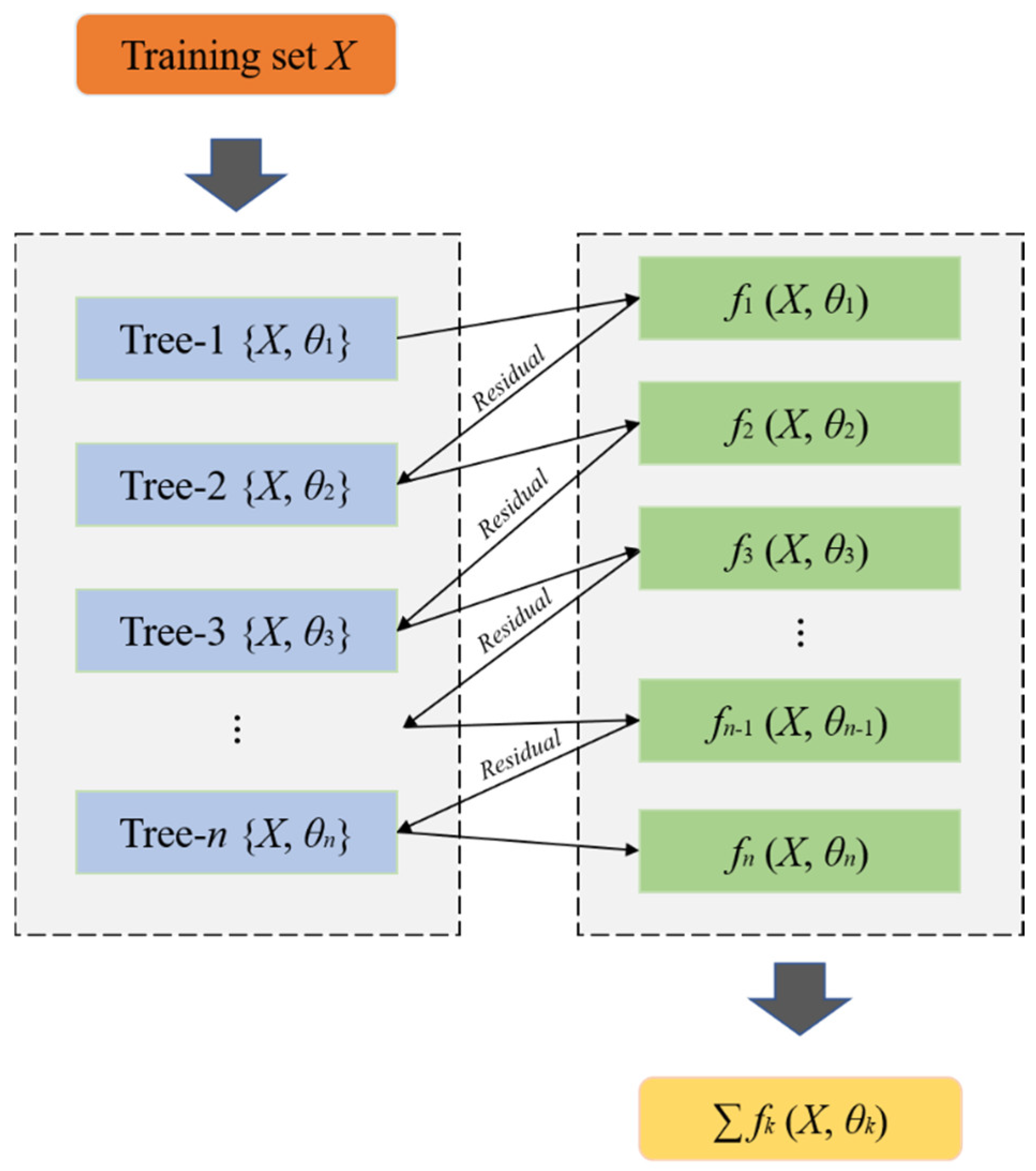
XGBoost is a boosting ensemble algorithm with a decision tree (DT) as the base learner that improves the classical gradient boosting decision tree (GBDT) algorithm [
48]. It is designed using an efficient, flexible, and portable distributed gradient boosting framework. Compared with GBDT, the calculation speed is faster while retaining excellent performance. The flowchart of this algorithm is indicated in
Figure 1. The core principle of XGBoost is to build DTs one after another and train the subsequent DT with the residuals of the previous ones. The values computed by all the constructed DTs are integrated to achieve a better result. It has been regarded as an advanced evaluator with ultra-high performance in both classification and regression [
21]. The XGBoost algorithm is explained as follows:
where
denotes the final model,
is the previous model,
represents the features corresponding to the sample
i,
is the newly generated DT model, and
t is the total number of DT models.
The objective function of the ensemble algorithm is an alternative. In order to avoid overfitting and improve iteration efficiency, XGBoost introduces model complexity to measure the computational efficiency [
49]. Accordingly, the objective function of XGBoost can be given by:
where
is the actual value,
is a convex loss function describing how well the model fits with training data, and
is the penalty term for regularization to avoid overfitting.
Gradient statistics are applied to the loss function, which effectively eliminates constant parameters. The simplified objective function is obtained as follows:
where
and
are the first and second order gradient statistics of the loss function, respectively. The penalty term
is evaluated by:
where
α and
λ are regularization parameters, whose default values are 1 and 0, respectively,
T is the number of leaf nodes controlled by the parameter
γ, and
w denotes the corresponding weight of the leaf nodes.
2.2. Random Forest Algorithm
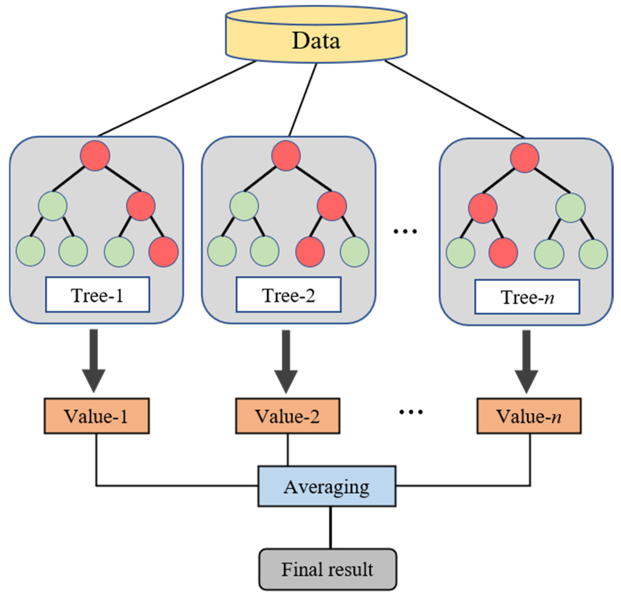
RF is a bagging ensemble algorithm with DT as the base learner [
50]. Its principle diagram is shown in
Figure 2. Different DTs are constructed to set up a forest by extracting sample and feature subsets from the original data. It is a stochastic process that ensures the independence of each DT, which improves the generalization capacity and avoids overfitting [
51]. Moreover, all constructed DTs tend to grow freely without pruning, which makes the construction process of each DT fast and the computational efficiency of RF improved. By integrating the results generated by all constructed DTs, the voting (for classification problems) or averaging (for regression problems) approach is used to determine the final results [
21]. According to the type of output variable in this paper, the RF algorithm is explained as follows:
where
represents the predicted value of the RF model,
is the predicted value of each DT, and
T represents the number of constructed DTs.
2.3. Dwarf Mongoose Optimization
The DMO algorithm is a swarm intelligence optimization algorithm that simulates the seminomadic life of dwarf mongoose in nature. The dwarf mongooses are known for foraging and scouting as a unit, and the DMO algorithm finds the optimal solution by simulating their social behavior. The DMO algorithm divides the swarm into three groups: the alpha group, the scout group, and the babysitter group [
47,
52,
53].
Firstly, the alpha group leads the scout group to forage and scout for a new sleeping mound, leaving the babysitters group to take care of the young dwarf mongooses in the old sleeping mound. Secondly, when a food source is not found, the alpha and scout groups will go back to the old sleeping mound to exchange members with the babysitter group. Thirdly, the alpha group continues to go out foraging and scouting for new sleeping mounds. The family returns intermittently to exchange babysitters and repeats the cycle until a food source is found.
The process of DMO for hyperparameter tuning can be broken down into the following steps [
47]:
(1) Initialization: The DMO algorithm starts by initializing the population of solutions as follows:
where
X is the set of current candidate populations,
n denotes the population size, and
d is the dimension of the problem. These solutions represent different sets of hyperparameters for the XGBoost and RF models.
(2) Objective function: The DMO algorithm requires an objective function that quantifies the performance of each solution. In this study, the average root mean squared error (RMSE) values of five-fold cross-validation (CV) were employed as the fitness function. The foraging behavior of the dwarf mongoose is mimicked by dividing the population into alpha, scout, and babysitter groups. The probability of each individual becoming alpha is computed by:
where
fiti denotes the fitness value of the
i-th individual.
(3) Behavior of dwarf mongooses: In the optimization of the DMO process, these dwarf mongooses work together to find food and a new sleeping mound. The movement of dwarf mongooses is determined by the leader of its subgroup. Their movement is based on the position of the alpha and the current position of the solution, which is calculated as follows:
where
Xi is the position of the alpha group, and
smi denotes the current position of the solution.
(4) Cooperative search: DMO encourages a cooperative search among the solutions in the population. This means that solutions collaborate and share information to improve the overall performance of the population. In the context of hyperparameter optimization, it implies that solutions with promising hyperparameters influence or guide other solutions towards better hyperparameter configurations.
(5) Communication and information sharing: In DMO, solutions share information about their performance and hyperparameters with others. This communication helps the population converge toward better solutions.
(6) Update hyperparameters: Based on the cooperative search and shared information, the hyperparameters of each solution are updated.
(7) Fitness evaluation: After updating the hyperparameters, the fitness of each solution is re-evaluated using the objective function. Solutions that perform better are favored and contribute more to the cooperative search process.
(8) Termination: The algorithm terminates when a stopping criterion is met.
(9) Final solution selection: Once the optimization process concludes, the solution with the best-performing hyperparameters, according to the objective function, is selected as the final model configuration.
2.4. Model Evaluation Metrics
In this study, four metrics were employed to assess the performance of the proposed models, including the coefficient of determination (
R2 score), the RMSE, the mean absolute error (MAE), and the variance accounted for (VAF). RMSE and VAF are maximization performance metrics, while MAE and VAF are minimization performance metrics [
54].
R2 score represents the proportion of the squared correlation between the predicted and actual values of the target variable, which can be calculated by:
where
indicates the actual value,
indicates the predicted value of the model, and
represents the average of the actual values.
RMSE represents the standard deviation of the fitted error between the predicted value and the actual value, which can be calculated by:
where
n indicates the total number of samples.
VAF characterizes the prediction performance by comparing the standard deviation of the fitted error with the standard deviation of the actual value, which is defined as:
where var indicates the variance.
MAE represents the average error between predicted value and actual value, which can be calculated by:
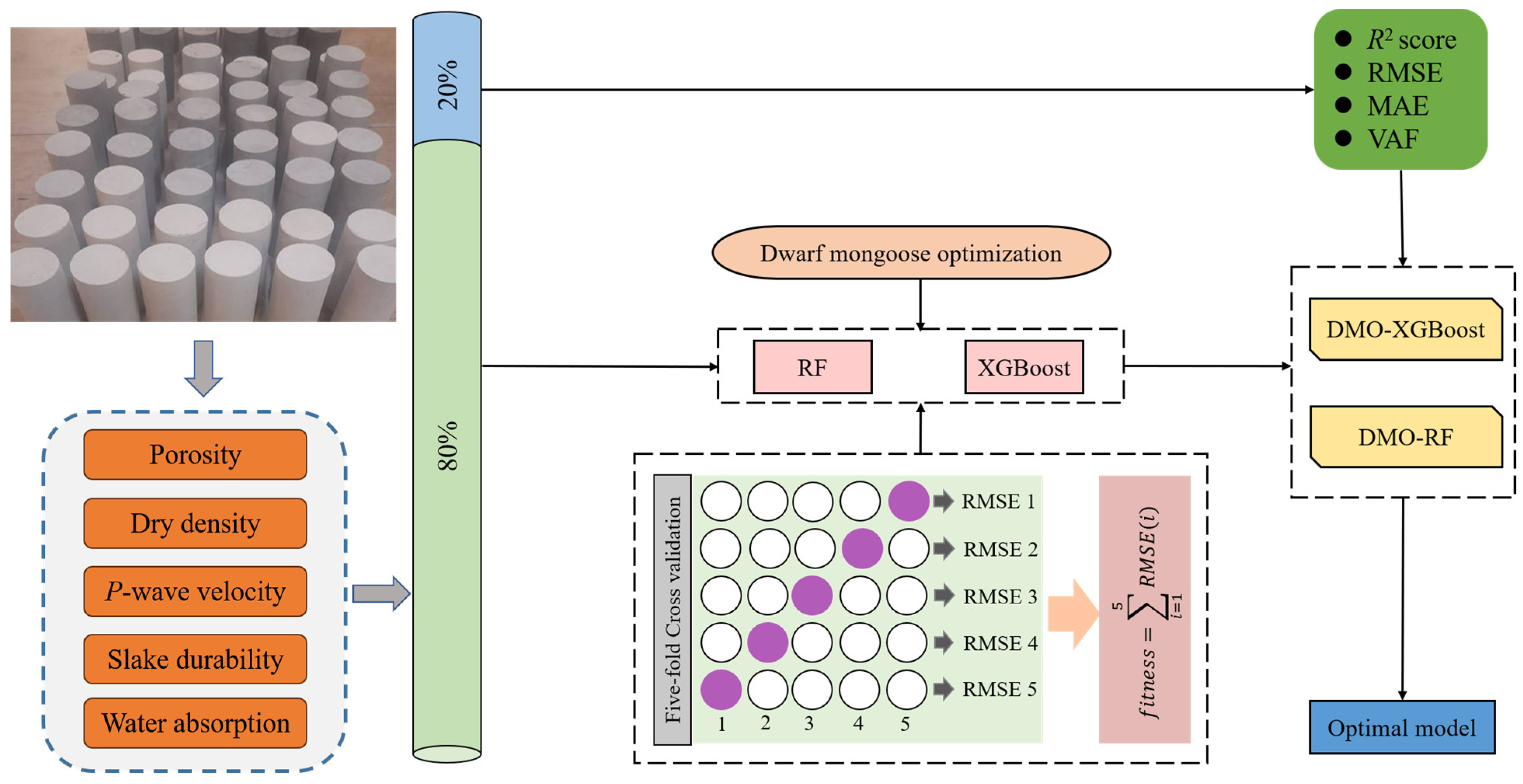
2.5. Proposed Approach
In this study, two novel hybrid ensemble learning models were proposed to estimate the
E of rock by optimizing the XGBoost and RF models through the DMO algorithm. The structure of the proposed approach is indicated in
Figure 3. Firstly, a database including 90 rock samples with five indicators was established. Secondly, 80% of the samples were utilized for training, while the remaining 20% were reserved for testing [
55]. Thirdly, to validate the superiority of the proposed hybrid ensemble learning models, a comparison against default XGBoost and RF models was performed. Finally, the
R2 score, RMSE, MAE, and VAF were adopted to evaluate the performance of models on the test set.
The XGBoost and RF algorithms were implemented on the Python library “sci-kit-learn” [
56], and the DMO algorithm was implemented on the Python library “MELPY” [
57,
58]. All experiments were processed using a Windows 10, 64-bit computer with 8 Gb of RAM running an Intel
® Core™ i7-9700F CPU @ 3.00 GHz × 2.
3. Data and Variables
According to the work of Abdi et al. [
25], four types of rocks, including marl, siltstone, claystone, and limestone, were collected and cored in the laboratory to obtain standard core samples. A total of 90 rock samples were obtained for conducting physical tests and developing
E-estimation models. Among the 90 samples, each set of data contains five indicators, including porosity (
A1), dry density (
A2),
P-wave velocity (
A3), slake durability (
A4), and water absorption (
A5). Among them, porosity (
A1) is an important factor in determining the strength and deformation behavior of rock, and water absorption (
A5) is related to porosity. Dry density (
A2) and
P-wave velocity (
A3) are two common petrophysical properties related to the
E of rock. Yagiz et al. [
28] found that slake durability (
A4) cycles have a significant effect on the prediction of UCS and modulus of elasticity for carbonate rocks. It is important that these five indicators can be conveniently measured in the laboratory, and therefore, they were selected as input indicators. The detailed descriptions of these indicators are displayed in
Table 2, and the statistics of the dataset are illustrated in
Table 3.
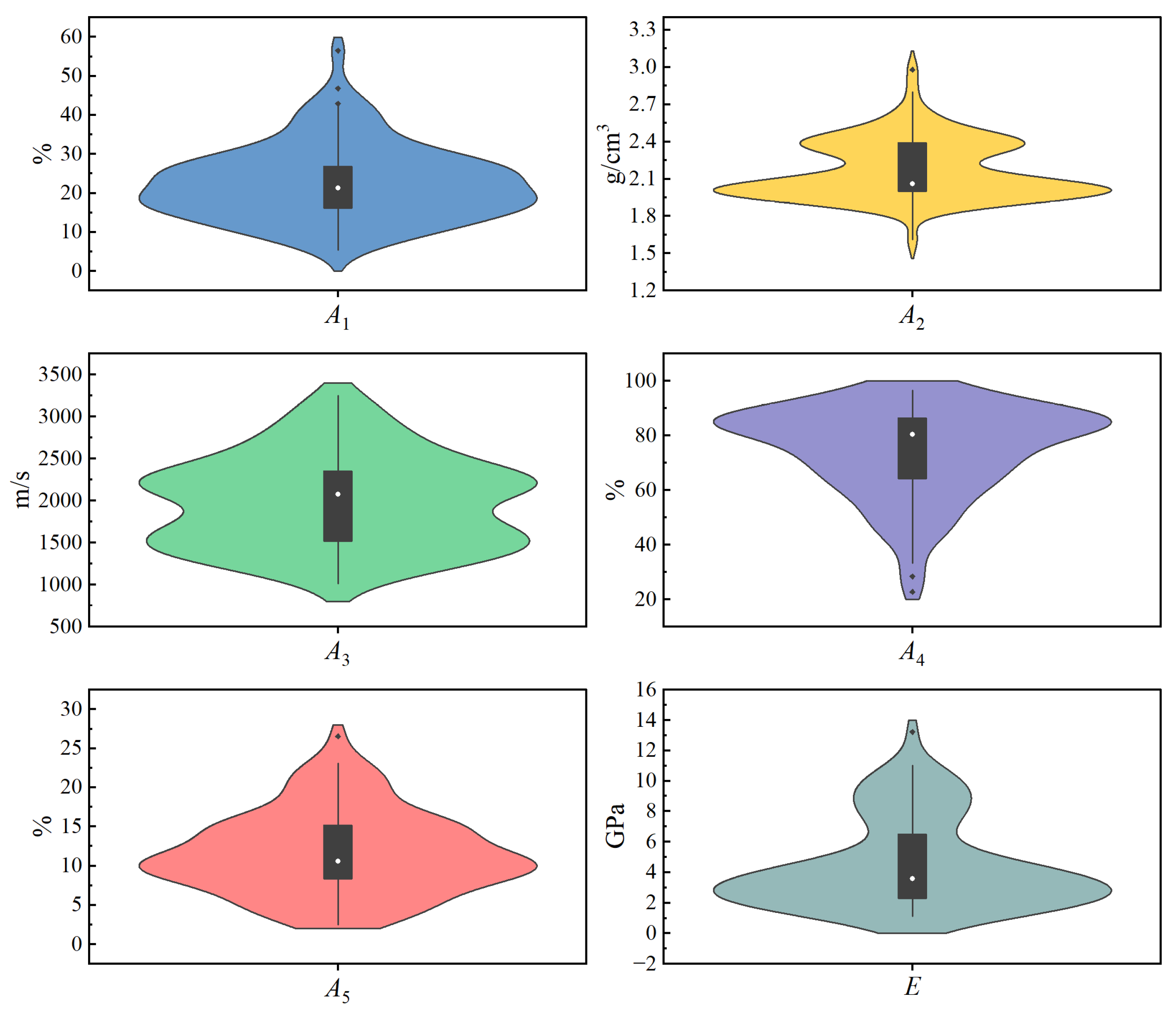
The violin plots of the five indicators and
E are shown in
Figure 4. These plots are a combination of box plots and density plots, offering insights into the overall distribution of the dataset. In each violin plot, the white dot at the center represents the median of the samples, the upper and lower extents of the thick black line denote the third and first quartiles of the samples, the top and bottom of the thin black line indicate the upper and lower adjacent values, and the black dots are outliers. From
Figure 4, it can be seen that the distribution of all the data is relatively balanced, but there are some outliers, which indicates the complexity of estimating the
E of rock.
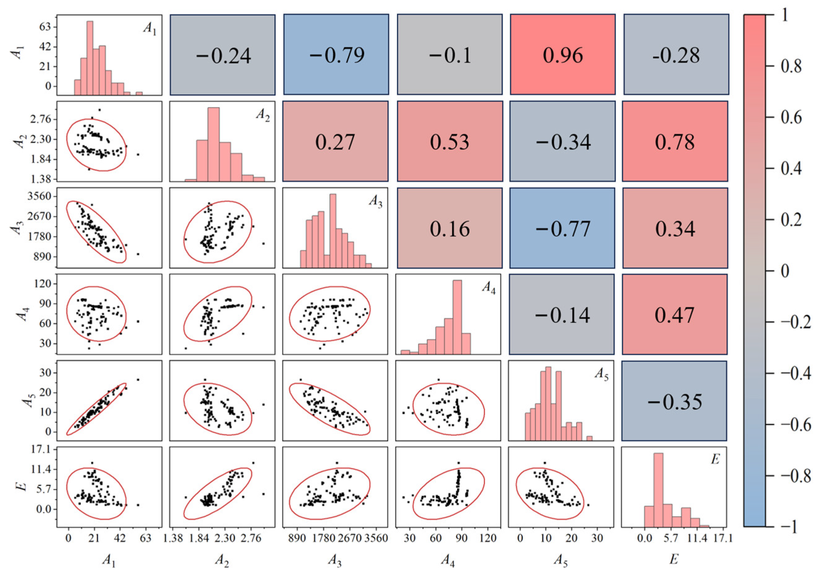
To visualize the distribution of this dataset, the correlation pair plots and heatmap of the Pearson correlation coefficient between indicators and
E are displayed in
Figure 5. The results show that
A2,
A3, and
A4 are positively correlated with
E, while others are negatively correlated. Among them, the strongest correlation was found between
A2 and
E with an absolute value of the correlation coefficient of 0.78, and the weakest correlation was found between
A1 and
E with an absolute value of the correlation coefficient of 0.28.
5. Discussion
5.1. Comparison with Different Classical Hybrid Models
To verify the effectiveness of the proposed DMO algorithm, the classical simulated annealing (SA) and Bayesian optimization (BO) algorithms were introduced to optimize the RF and XGBoost models for comparison [
62,
63,
64,
65]. The evaluation metrics of the SA-RF, SA-XGBoost, BO-RF, and BO-XGBoost models in the training and testing phases are shown in
Table 6.
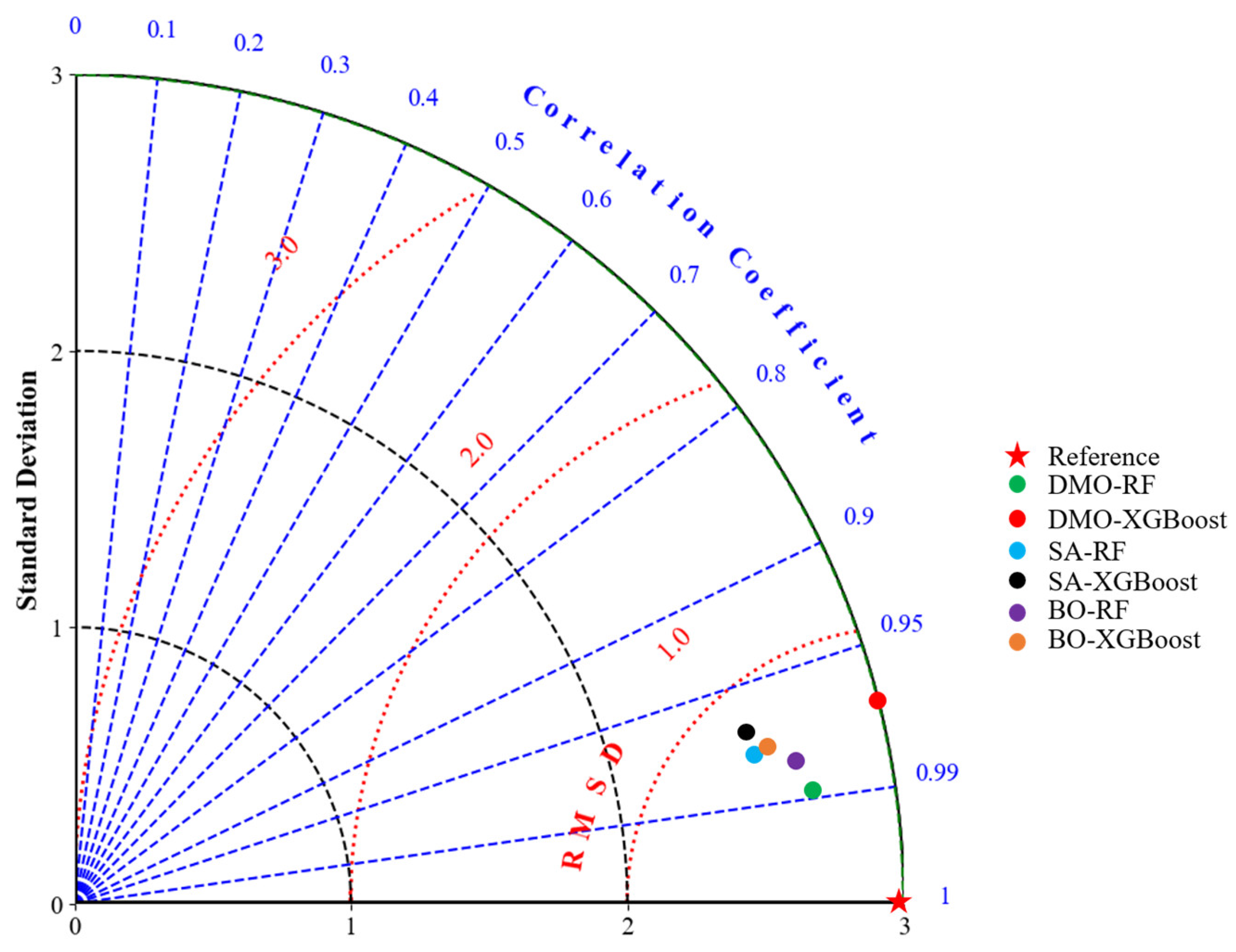
To compare the developed models more visually, the Taylor diagram was plotted, as seen in
Figure 8. A complete Taylor diagram consists of three components: standard deviation (SD, black and green dashed line), root mean square deviation (RMSD, red dashed line), and correlation coefficient (CC, blue dashed line) [
66]. The red pentacle in
Figure 8 was the reference point, which represents the actual
E values, and the scatters represent the different prediction models. The scatter with the closest distance to the reference point (with the lowest RMSD value) corresponds to the optimal prediction model. The SD, RMSE, and CC values of all scatters are calculated in
Table 7. It can be seen that the DMO-RF model was the best model that was closest to the reference point with an RMSD of 0.530, followed by the BO-RF, DMO-XGBoost, BO-XGBoost, SA-RF, and SA-XGBoost models.
5.2. Comparison with Other ML Models
To confirm the performance of the developed models, three other ML models were introduced for comparison, namely the SVM, decision tree (DT), and multilayer perceptron neural network (MLPNN). The hyperparameters of these models were default. In addition, Adaptive boosting machine (Adaboost) and Category gradient boosting machine (CatBoost) methods were developed by Abdi et al. [
25] on the same dataset. Furthermore, to visually compare the seven ML models, a scoring system was implemented to give corresponding scores to each model [
67]. The values and scores of all models on four evaluation metrics are calculated in
Table 8. It can be seen that the overall score ranking for all models is DMO-RF (28) > DMO-XGBoost (24) > CatBoost (20) > Adaboost (16) > SVM (12) > MLPNN (8) > DT (4).
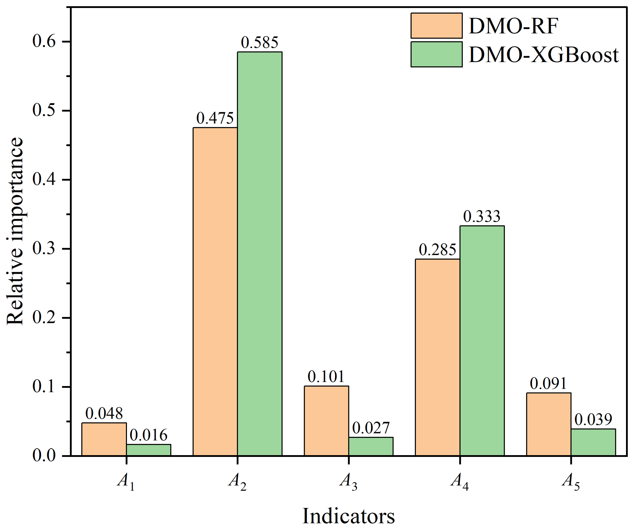
5.3. Relative Importance of Indicators
In this study, the relative importance of each indicator was determined by combining the DMO-RF and DMO-XGBoost models with the permutation feature importance technique, which is indicated in
Figure 9 [
68,
69]. Based on the DMO-RF model, the rank of the indicators’ importance was
A2 >
A4 >
A3 >
A5 >
A1. According to the DMO-XGBoost model, the rank of the indicators’ importance was
A2 >
A4 >
A5 >
A3 >
A1. The results were consistent with the calculations of the feature importance analysis module built into the XGBoost and RF models. Apparently, two indicators were the most important:
A2 (dry density) and
A4 (slake durability). The results can be used as a reference for developing more reliable
E estimation models of rock in the future.
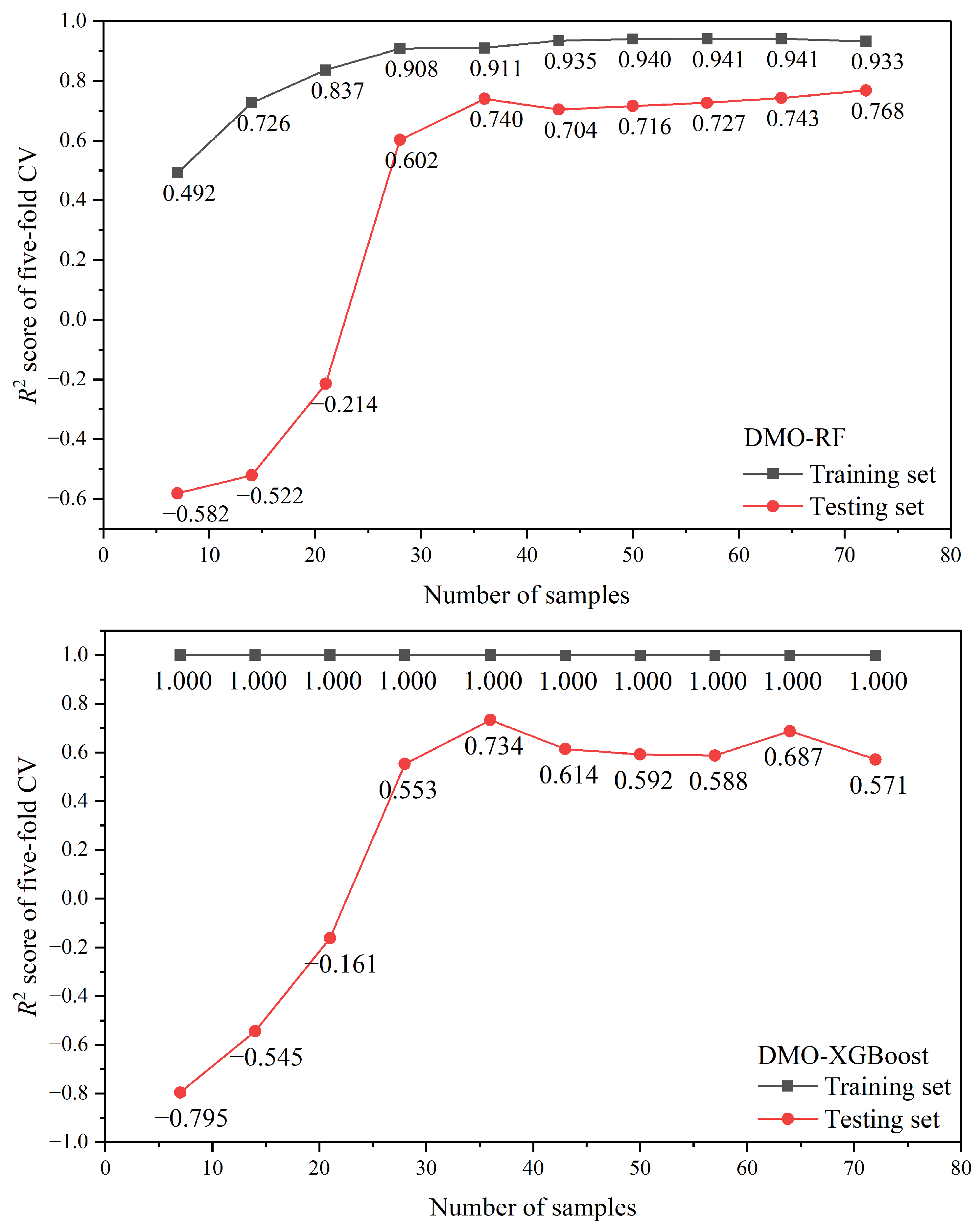
5.4. Overfitting Validation
Furthermore, to further analyze whether the proposed DMO-RF and DMO-XGBoost models suffered from overfitting or underfitting, the convergence curves are plotted in
Figure 10. The horizontal axis represents the number of samples, while the vertical axis represents the
R2 score obtained through a five-fold CV. It can be seen that the DMO-RF and DMO-XGBoost models tended to converge as the sample size increased. However, the DMO-RF model performed with less error between the training and test sets than the DMO-XGBoost model, which indicates that the proposed DMO-RF model effectively mitigated the issue of generalization error and exhibited a certain degree of resistance against overfitting.
5.5. Limitations
Although the proposed hybrid ensemble approaches obtained excellent results in estimating the E of rock, there are still some limitations to consider:
(1) The dataset used in this study is relatively small, and the specimens in the original dataset were composed of four types of weak rocks, including marl, siltstone, claystone, and limestone. There is no consideration of other types of rock, such as granite, basalt, and other hard rocks. This situation might lead to the presence of a sampling bias that might affect the generalizability of the proposed ML models. Therefore, it is crucial to expand the database by collecting various types of rock cases to increase the quantity and quality of the dataset.
(2) More indicators should be considered. Although the five indicators in this study affect the E of rock significantly, other factors such as depth of coring, mineral composition, grain size distribution, and RQD index also have an effect on the E of rock. It is valuable to explore the influences of these indicators on the E of rock estimation.
Although the aforementioned limitations exist, the developed DMO-XGBoost and DMO-RF models in this study could be considered a feasible and practical tool for estimating the E of rock. Compared to traditional expensive and time-consuming laboratory testing methods for rock mechanical parameters, the proposed models have potential advantages in terms of cost savings and time efficiency. Geotechnical engineers can significantly reduce the need for costly laboratory testing, providing project budget savings while enabling faster and more effective assessment of geologic and geotechnical risks. In addition, the developed models could be extended to estimate other geotechnical parameters, such as UCS, rock shear strength, and rock brittleness, et al.
6. Conclusions
E is one of the important parameters in rock mechanics. Accurately estimating the E of rock is significant for the design and construction of geotechnical projects. In this study, DMO-XGBoost and DMO-RF models were developed to estimate the E of rock. The effectiveness of the proposed models was verified using a database including 90 rock samples with five indicators. To avoid overfitting or selection bias, the five-fold CV method was combined with the DMO algorithm to tune the hyperparameters on the training set (80% of the dataset). The R2 score, RMSE, MAE, and VAF were adopted to evaluate the performance of models on the test set (20% of the dataset). In addition, two default ensemble models (XGBoost and RF) were introduced and compared with the proposed two hybrid models. Overall, the DMO algorithm improved the predictive performance of the default XGBoost and RF models, and the DMO-RF model performed best with an R2 of 0.967, RMSE of 0.541, MAE of 0.447, and VAF of 0.969 on the test set. Furthermore, the classical SA and BO algorithms were introduced to optimize the RF and XGBoost models for comparison, and the Taylor diagram was plotted to determine the comprehensive rank, which was DMO-RF > BO-RF > DMO-XGBoost > BO-XGBoost > SA-RF > SA-XGBoost. The permutation feature importance technique revealed that dry density and slake durability were more influential than other indicators in the evaluation results. Based on the convergence curves, it was verified that the DMO-RF model can reduce the generalization error and avoid overfitting.
In future work, a larger dataset containing higher-quality data should be established to improve the estimation performance. In conclusion, the proposed DMO-RF model in this paper can be considered a viable and useful tool in estimating the E of rock and can be recommended for the application of other geotechnical parameter estimations, such as UCS, rock shear strength, and rock brittleness, amongst others.


