Abstract
Knowledge graphs (KGs) have gained prominence for representing real-world facts, with queries of KGs being crucial for their application. Aggregate queries, as one of the most important parts of KG queries (e.g., “ What is the average price of cars produced in Germany?”), can provide users with valuable statistical insights. An efficient solution for KG aggregate queries is approximate aggregate queries with semantic-aware sampling (AQS). This balances the query time and result accuracy by estimating an approximate aggregate result based on random samples collected from a KG, ensuring that the relative error of the approximate aggregate result is bounded by a predefined error. However, AQS is tailored for simple aggregate queries and exhibits varying performance for complex aggregate queries. This is because a complex aggregate query usually consists of multiple simple aggregate queries, and each sub-query influences the overall processing time and result quality. Setting a large error bound for each sub-query yields quick results but with a lower quality, while aiming for high-quality results demands a smaller predefined error bound for each sub-query, leading to a longer processing time. Hence, devising efficient and effective methods for executing complex aggregate queries has emerged as a significant research challenge within contemporary KG querying. To tackle this challenge, we first introduced an execution cost model tailored for original AQS (i.e., supporting simple queries) and founded on Taylor’s theorem. This model aids in identifying the initial parameters that play a pivotal role in the efficiency and efficacy of AQS. Subsequently, we conducted an in-depth exploration of the intrinsic relationship of the error bounds between a complex aggregate query and its constituent simple queries (i.e., sub-queries), and then we formalized an execution cost model for complex aggregate queries, given the accuracy constraints on the error bounds of all sub-queries. Harnessing the multi-objective optimization genetic algorithm, we refined the error bounds of all sub-queries with moderate values, to achieve a balance of query time and result accuracy for the complex aggregate query. An extensive experimental study on real-world datasets demonstrated our solution’s superiority in effectiveness and efficiency.
Keywords:
simple aggregate query; complex aggregate query; execution cost model; knowledge graph; multi-objective optimization; effectiveness and efficiency trade-off; genetic algorithm; Taylor’s theorem; normal equation; CentOS workstation; JAVA; Python MSC:
68W25
1. Introduction
In 2012, Google introduced the concept of knowledge graphs (KG), to manage large amounts of real-world information, represented as a comprehensive graph.In this graph, entities with attributes are denoted as nodes, while relationships between entities are represented as edges. KGs play a pivotal role in various applications, including intelligent search, question answering, and semantic search [1,2]. KG queries stand out as a fundamental component of the above applications and have been widely studied in the literature. They can be divided into two categories, according to the query type. At the beginning, KG queries primarily focused on addressing the factoid query problem. Factoid queries were defined as enumerations of noun phrases [3], such as “Find all cars produced in Germany”. A common technique for answering factoid queries is a graph query [4,5,6,7,8,9]. This approach involves constructing a query graph to represent the user’s intent and identifying exact or approximate matches with the query graph within the KG. Recently, there has been growing interest in extracting statistical insights from these entity sets. For instance, the aggregate query [10] “What is the average price of cars produced in Germany?” aims to calculate the average price of all automobiles linked through the semantic relation “product” to the specific entity “Germany”. Notably, it was observed that 31% of queries in the real query log LinkedGeoData13 and 30% of queries in WikiData17 were identified as aggregate queries [11].
- Existing solutions. A straightforward method for handling aggregate queries for KGs is to perform additional aggregate operations on the answers returned by factoid queries. The effectiveness of this method depends on the quality of answers provided by the factoid queries. In addition, this method tends to overlook answers with equivalent meanings but differing structures [4,6,9,12,13,14,15], thus resulting in inaccurate results. The concept of an "accurate" answer is often contingent upon the user’s query intent and may even be inherently ambiguous [16,17]. Moreover, this still suffers from the inefficiency issue, due to the extra time required to run additional aggregate operations. Therefore, the method of approximate aggregate queries with semantic-aware sampling (AQS) [18,19] was proposed to tackle the issues encountered above. It utilizes a random walk based on KG embedding to collect high-quality random samples through semantic-aware sampling and calculates approximate aggregate results based on random samples using the bag of little bootstraps (BLB) method. It returns a confidence interval regarding the approximate result and ensures that the relative error of the approximate result is bounded by a predefined error bound. We discuss this in Section 2 in more detail. AQS performs well for simple aggregate queries of KGs, in both effectiveness and efficiency. However, it cannot be directly extended to complex aggregate queries of KGs. Here, we call an aggregate query of a KG G (e.g., How many cars are produced in Germany?, see Figure 1, middle left part), which is simple if formed as a query graph Q with only one specific entity (e.g., Germany) and a predicate (e.g., product), and this aims to find the aggregate results for an attribute (e.g., the aggregate function = COUNT for a wildcard attribute ∗) of target entities (e.g., cars) that are semantically related to the given specific entity following the specific predicate. We call a query complex if it is a combination of a set of simple aggregate queries (i.e., sub-queries). In Section 2, we formally define simple and complex aggregate queries. The reason why AQS cannot adapt to complex queries comes from the fact that even if each sub-query satisfies the predefined error bound (guaranteed by performing AQS for each sub-query), the accuracy of the complex query may still not be guaranteed. We next show this problem of AQS clearly.
- Efficiency vs. effectiveness trade-off problem. In AQS, efficiency refers to the response time of a query, and effectiveness (or accuracy) refers to the relative error of the approximate aggregate result regarding the ground truth. Intuitively, the accuracy of a complex query can be guaranteed if we set quite a small predefined error bound for each sub-query of the complex query. However, this would significantly increase the response time, as the AQS would require more time to collect additional samples to achieve a good approximate aggregate result. This creates an efficiency vs. effectiveness trade-off problem for complex aggregate queries using AQS. More precisely, the essence of this problem is how to configure appropriate predefined error bounds for each sub-query, so that the complex query’s accuracy is guaranteed and its response time is as short as possible. We clarify this in the following two examples.

Figure 1.
Simple and complex aggregate queries on a knowledge graph (taking DBpedia as an example).
Figure 1.
Simple and complex aggregate queries on a knowledge graph (taking DBpedia as an example).

Example 1.
Effectiveness issue. Considering the complex aggregate query “how many times the number of cars produced in Germany is that in China?” with two sub-queries (see Figure 1, top part). This consists of two sub-queries: “how many cars produced in Germany” (ground truth in DBpedia and aggregate function is COUNT) and “how many cars produced in China” (ground truth in DBpedia and aggregate function is COUNT). The ground truth of is . With a predefined error bound for , the aim is to ensure the relative error of the approximate result of remains within . Setting appears straightforward ( and are predefined error bounds for sub-queries), yielding and for and , respectively. Although the relative error of each remains within its own (e.g., for and for ), the relative error of ’s approximate result ( and ) exceeds the specified , leading to an accumulation of errors. Worse still, the relative error of the final aggregate result may increase with an increasing number of sub-queries in a complex query.
To address this, a simple method is to set an smaller than e for each sub-query to obtain more accurate sub-query results, thus minimizing the relative error of . However, this raises another efficiency issue, which we show below.
Example 2.
Efficiency issue.Given for two sub-queries, we obtain two approximate aggregate results using AQS as and . The relative error of each sub-query’s aggregate result remains within , and the relative error of the complex query’s aggregate result is . However, this configuration results in a significant increase in the querying time for each sub-query. The response time of in this case is 1253.97 ms. Compared to the time (797.52 ms) consumed in the case of Example 1, simply reducing the error bounds e for all sub-queries from 1% to 0.5% resulted in a 57.2% increment in the response time. The smaller the sub-query’s error bound , the longer the response time of a complex query. This is because we need to collect more representative samples to refine the approximate aggregate result of each sub-query.
In summary, configuring appropriate error bounds for sub-queries is crucial for achieving a trade-off between the effectiveness and efficiency of complex aggregate queries when using AQS.We next briefly show our solution using the problem–solution tree illustrated in Figure 2.
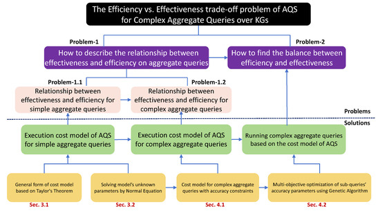
Figure 2.
Problem–solution tree of the effectiveness vs. efficiency trade-off problem and our solution.
- Our solution and contributions. As shown in Figure 2, we focus on the effectiveness vs. efficiency trade-off problem of AQS for aggregate queries of KGs. We start with the preliminaries of AQS and formally define this problem in Section 2. To solve it, we first study the relationship between effectiveness and efficiency on aggregate queries for KGs (Problem-1), then we leverage this relationship to achieve a balance between the two (Problem-2). For Problem-1, we first study the relationship between effectiveness and efficiency for simple aggregate queries (Problem-1.1), then we extend this to complex aggregate queries (Problem-1.2). To solve Problem-1.1, in Section 3, we first present a cost model of AQS for simple aggregate queries on the basis of Taylor’s theorem (Section 3.1). Then, we show how to determine the parameters of this cost model using a normal equation (Section 3.2). Next, we solve Problem-1.2 by exploring the relationship between the sub-query error bound and the complex aggregate query error bound, establishing a general form of the execution cost model for complex aggregate queries, with accuracy constraints given the relationship of the error bounds (Section 4.1). Finally, in Section 4.2, we employ a multi-objective optimization genetic algorithm to determine the optimal error bounds for sub-queries, thus minimizing the total response time for a complex aggregate query, while returning a sufficiently accurate approximate aggregate result for the complex query. In the context of simple aggregate queries, our approach using a cost model for AQS exhibited 1.8X efficiency improvement, on average, compared to the original AQS without the cost model. For complex aggregate queries, our method stands as the sole solution capable of meeting predefined user error bounds, while maintaining a commendable level of efficiency.
- We present an execution cost model for AQS based on Taylor’s theorem and obtain appropriate parameters for this cost model using the normal equation.
- We extend the cost model of AQS to complex aggregate queries, associated with a set of accuracy constraints on the complex aggregate queries, as well as the relationship between the sub-query error bound and complex query error bound.
- We leverage a genetic algorithm to determine the optimal error bounds for sub-queries, achieving a balance between efficiency and accuracy.
- We conducted experiments with three widely used real-world KGs, to demonstrate the effectiveness and efficiency of our method.
2. Preliminaries
We first provide the preliminaries and then formalize the problem studied in this paper. Frequently used notations are summarized in Table 1.

Table 1.
Frequently used notations.
Definition 1.
Knowledge Graph. defines the knowledge graph (KG), where a finite set of nodes V and a set of edges are encompassed. (1) An entity is represented by a node , and the relationship between two entities is denoted by an edge . (2) Names and various types are assigned to each node using the label function L, while each edge is associated with a predicate. (3) A set of numerical attributes denoted as are possessed by each node , and the value of the numerical attribute of u is indicated by .
Example 3.
A unique name and at least one type are possessed by each node u in a KG G. In Figure 1, the name = and the type = are held by the entity . Additionally, a set of numerical attributes, such as = , , are associated with it. Furthermore, the predicate = is associated with the edge . The value corresponding to the value attribute a of node u can be represented as . For instance, = 245.
We start with a simple aggregate query, which is defined in the query graph for a simple question—one of the most common questions [20,21], involving a single specific entity and a single predicate, taking the target entities as the answers [22]. We first obtain the execution cost model for the simple aggregate query, then we use it to form the model for complex aggregate queries.
Definition 2.
Simple aggregate query. defines the simple aggregate query over a KG G, where Q is the query graph used for candidate answer retrieval from G, and represents the aggregate function applied to the numerical attribute a of the answer to Q (considering three widely used non-extreme aggregate functions .). The query graph consists of a query node set , an edge set , and a label function . For a simple question, the query node set comprises two nodes, with representing a specific node and denoting the target node. The types and name are known for , whereas only the types are known for . Additionally, the edge set contains one edge with a predicate .
In this paper, we consider a complex aggregate query having multiple sub-queries as a complex aggregate query, such as star queries [23].
Definition 3.
Complex aggregate query. We define a complex aggregate query for G as , where (1) is a set of simple aggregate queries , each of which is defined as in Definition 2, constituting , (2) represents a user-defined function (UDF) for the results of all the simple aggregate queries, combining arithmetic operations such as and /.
Example 4.
Figure 1 illustrates that the query graph Q for the simple question “How many cars are produced in Germany?” contains a specific node (type: , name: ), a target node (type: ), and an edge (predicate: ). Additionally, is defined as for the wildcard attribute . Furthermore, the complex question “How many times the number of cars produced in Germany is that in China?” consists of two simple queries, and , with the aggregate function defined using the aggregate results () of and for the wildcard attribute .
- Approximate aggregate queries with semantic-aware sampling (AQS) [18] has recently been developed as an efficient and effective solution for answering simple aggregate queries for KGs, and it is briefly described as follows. When a simple aggregate query is posed for a KG G, the process of AQS comprises three main steps: (1) Semantic-aware sampling. A semantic-aware online sampling algorithm based on random walk for G is employed by AQS to gather answers from G, forming a random sample that likely represents entities with semantic similarity to the query graph Q. (2) Correctness validation of a random sample. AQS uses a greedy algorithm to filter the correct answers from the random sample, where a correct answer is defined as one with a semantic similarity greater than a predefined threshold . (3) Estimation and accuracy guarantee. With the random sample in hand, AQS estimates an approximate aggregate result . Subsequently, an accuracy guarantee for is provided by iteratively computing a tight confidence interval CI at a high confidence level , with representing the half-width of the CI (also known as the margin of error). This CI indicates that the ground truth V is covered by the interval with a probability of . We terminate AQS when the condition is satisfied, showing that the relative error of regarding V has an upper bound of e with a probability of (Theorem 2 in [18]).
Given the above definitions, the following problem captured our interest: an accurate execution cost model for AQS for complex aggregate queries of KGs needs to be designed. Typically, as the predefined error bound e decreases, the query time of AQS (or the execution cost) increases. An underlying relationship exists between the query time and e, and we aimed to derive this relationship to formulate our execution cost model.
Problem 1.
Given a complex aggregate query , we aimed to: (1) collect training data for the execution cost (i.e., running time) t regarding the independent variable x (e.g., x is the predefined error bound e, etc., and and are the observations of t and x), by running AQS, and (2) deriving the execution cost of AQS for regarding x by using D, as follows:
In Equation (1), the execution cost of the complex aggregate query is denoted as . This cost is composed of the individual costs of each simple aggregate query , represented as , where our execution cost model estimates . In Section 3, the independent variables that may affect the efficiency of AQS, such as the predefined error bound e, are discussed. To minimize the error between and the exact cost t with respect to the specific variable x, we adopt the mean squared error (MSE) as the loss function . This paper focuses on providing a solution to deriving the execution cost model for a specific complex aggregate query . It should be noted that different queries have distinct cost models (as explained in Section 3.1). In Section 4, we explore how to utilize the obtained cost model for a particular query, to formulate a universal cost model applicable to all queries (e.g., using the average as a simple method).
3. Execution Cost Model of AQS for Simple Aggregate Queries
In this section, the execution cost model for a simple aggregate query is studied, where the execution cost of a complex aggregate query is the sum of the cost of each sub-query. The relationship between the time consumed in each step of AQS [18] and the predefined error bound e is analyzed. Subsequently, a general form of the cost model is presented based on Taylor’s theorem in Section 3.1. Finally, in Section 3.2, the training data are collected, and the normal equation is applied, to determine the unknown parameters of the cost model, thereby providing an execution cost model for .
3.1. Execution Cost of AQS
As mentioned in Section 2, AQS consists of three main steps, thus the total execution cost of AQS for a simple aggregate query involves three parts. The execution cost of each step is next briefly analyzed (for detailed information on AQS, readers are referred to [18]), and then the Taylor’s theorem is used to approximate the cost of each step.
- Cost of semantic-aware random walk sampling. This step has three phases, where a query graph Q and a knowledge graph (KG) G are given. In the first phase, AQS finds the mapping node for the specific node that satisfies and . Afterward, a BFS is initiated from to extract an n-bounded subgraph with respect to , where each entity u from is within n hops from . In the second phase, AQS utilizes a KG embedding model (e.g., TransE [24]) to obtain the predicate similarity of each edge to the query edge . Consequently, AQS formulates a transition matrix based on the predicate similarities and performs random walk on until reaching convergence. Lastly, AQS employs the continuous sampling [25] technique to collect answers with greater semantic similarity to Q, forming a random sample S. Phases (1)–(2) are dedicated to random walk for , and the last phase is utilized for random sampling. Thus, the execution costs of phases (1)–(2) and phase (3) are denoted as and , respectively.
The above procedure establishes the relationship between and two factors: the size of and the convergence rate of random walk. The size of primarily depends on the mapping node corresponding to the specific node , because AQS restricts the consideration to the n-bounded subgraph with respect to , resulting in various sizes of for different . Conversely, the convergence rate of random walk is significantly influenced by the predicate of the query edge. Each different predicate in the query edge implies a distinct predicate similarity , which in turn leads to the formation of different transition matrices . Employing a random walk using distinct would consequently yield various convergence rates. For a specific simple aggregate query , the size of and the query edge’s predicate are predetermined, thus making a constant. Nevertheless, different queries exhibit different execution costs. Let us contemplate the following three queries:
- Q1: “How many cars are produced in Germany?”
- Q2: “How many Spanish football players are there?”
- Q3: “How many football players are there in Germany?”
Considering and , their n-bounded subgraphs differ due to the distinct specific nodes with the names and , respectively. Consequently, they exhibit a different . Moreover, considering and , they share the same n-bounded subgraph because of the identical with the name . However, the predicates of and differ ( and ), resulting in distinct transition matrices and, consequently, different values. In this paper, is treated as a constant for a particular query (we will discuss how to determine later in Section 3.1). Unlike , the execution cost is not a constant and depends on the size of the random sample (e.g., ) obtained through continuous sampling. Generally, a larger requires more for continuous sampling. Intuitively, a small predefined error bound e indicates that AQS needs more iterations to achieve a high-quality confidence interval, by collecting a larger random sample. Hence, the sample size is determined by the value of e, making essentially related to e, as shown in Equation (2), where the function estimates the sample size for a given e, and the function estimates based on the estimated sample size . We will present the general forms of and later in Section 3.1 and introduce the training procedure in Section 3.2.
- Cost of Correctness validation for the random sample. After obtaining a random sample S through semantic-aware random walk sampling, AQS employs a process of correctness validation to identify the correct answers within S. Subsequently, AQS can directly utilize these correct answers for approximate result estimation. In essence, correctness validation involves enumerating all answers in S, making its execution cost dependent on the sample size . Similarly to the execution cost mentioned earlier, can also be estimated as . In other words, a smaller predefined error bound e necessitates a larger sample size , thereby resulting in a longer time for correctness validation.
- Cost of estimation and accuracy guarantee. After validating a random sample S for correctness, AQS employs two unbiased estimators and one consistent estimator for , and , respectively, to estimate the approximate aggregate result for the query in the form of a confidence interval . Simultaneously, AQS provides a robust accuracy guarantee by iteratively refining until . Intuitively, a smaller predefined error bound e requires more iterations for refinement; thus, the execution cost of this step is dependent on e, and can be expressed as . In summary, we define .
- General cost model based on Taylor’s theorem. Based on the above analysis, we can derive the total execution cost of AQS as . Since both and are related to the sample size determined by the predefined error bound e, we can simplify T by combining and together as :where , which is a constant with respect to a particular query , can be obtained by running AQS multiple times for and computing the average query time. Since the relationship between the predefined error bound e and T is non-linear, estimating T becomes a non-linear regression problem. To address this problem, we utilize Taylor’s theorem [26] to present the general form of each unknown term in Equation (3) (e.g., and ). Taylor’s theorem provides an approximation of a n-times differentiable function around a given point using a polynomial of degree n (known as the n-th order Taylor polynomial). By applying Taylor’s theorem, the terms , , and can be approximated using the n-th order Taylor polynomials.
3.2. Cost Model Training
Given a particular aggregate query , our objective is to determine each term in Equation (3). To estimate the execution time , we repeatedly run AQS for and calculate the average time of , treating it as a constant in Equation (3). On the other hand, for and , we utilize the normal equation to estimate the parameters for a specific order n.
- Estimation of . To estimate , we perform only the first two phases of the first step in AQS, which involve constructing a n-bounded subgraph and performing the random walk until convergence. We repeat these phases for r times and calculate the average time as the estimation of for the given query , where is the running time of the i-th execution.
- Estimation of . To estimate the parameters for a given n-th order Taylor polynomial, such as Equations (4)–(6), we first collect a set of statistics during the runtime as the training data. Next, we use the normal equation to obtain the optimal solution that minimizes the mean squared error (MSE). The details are presented below.
- Collecting training data. The focus of our data collection is the relationships among the sample size , the predefined error bound e, and the execution cost of each step in AQS. We collect run-time statistics in the form of quadruples , where represents an observation of the independent variable e (with a random value in the range ), denotes the total size of the sample required by AQS for a specific , records the execution time of continuous sampling and correctness validation in AQS for , and represents the execution time for estimation and the accuracy guarantee in AQS for . To compile the training data, we generate m observations of e as in our implementation, resulting in m quadruples. Subsequently, we extract information from these statistics to formulate distinct training data for different n-th order Taylor polynomials and to estimate the parameters .
- (1) Training data for . Based on the analysis in Section 3.1, is directly influenced by the sample size , which is primarily determined by the predefined error bound e. Therefore, we initially collect a set of tuples as training data, to estimate the parameters for (Equation (4)). Subsequently, we gather another set of tuples as training data, to estimate the parameters for (Equation (5)). By substituting Equation (4) with the optimal and Equation (5) with the optimal , we can derive the final execution cost model for .
- (2) Training data for . As mentioned in Section 3.1, is associated with the predefined error bound e. Thus, we collect a set of tuples as training data to estimate the parameters for (Equation (6)).
- Training using the normal equation. For illustrative purposes, we will use as an example to explain the training process, which is identical for both and . Given the training data collected for , the training using the normal equation proceeds as follows:
(1) We first transform the non-linear Taylor polynomial of (Equation (6)) into a linear form by assuming , resulting in .
(2) We represent the parameters, features, and observed execution costs as an -dimensional column vector , an matrix X, and an m-dimensional column vector Y, respectively. We show X and Y as
where represents the n-order feature of the m-th observation , defined as , and corresponds to the m-th observation of the execution cost with respect to . (3) Finally, we employ the normal equation based on the MSE metric to solve for the parameters , as shown below.
4. Complex Aggregate Query Method Based on the Cost Model of AQS
In Section 3, we discuss the cost model of AQS for simple aggregate queries. It is natural that the total cost of a complex aggregate query is the sum of the cost of ’s sub-queries. Therefore, the goal of processing using the cost model of AQS is to determine the optimal error bound of each sub-query to minimize the total running time of , on the premise of satisfying the accuracy constrains on , i.e., ensuring the relative error of the final aggregate result of is bounded by the predefined e of . In this section, we first explore the relationship between the error bound of each sub-query and the error bound of the complex aggregate query and establish the accuracy constraints on complex aggregate queries based on such a relationship (Section 4.1). Then, we leverage a generic algorithm to obtain the optimal error bounds for sub-queries (Section 4.2).
4.1. Accuracy Constraints on Complex Aggregate Queries
From Definition 3, a complex aggregate query is composed of a set of sub-queries , is a UDF for all simple aggregate query results. Among them, each sub-query will obtain an approximate result through the AQS method, and the relative error of the approximate result is determined using the error bound of the sub-query . The larger , the greater the probability that the approximate result will deviate from the true value . Obviously, in order to make the result of satisfy the user-defined error bound e, the error bounds configured for all sub-queries must satisfy a certain accuracy constraint.
In [18], Wang et al. provided a theorem to show that, given a simple aggregate query with a computed confidence interval CI (the user-specific confidence level is ), if , then the probability of the relative error satisfying is . We next discuss how to leverage the above theorem to derive the accuracy constraint of . To be more precise, the error bound e for a complex aggregate query is guaranteed only if the accuracy constraint of holds. To achieve this, we start with a complex aggregate query consisting of two sub-queries, then provide the general form of the accuracy constraints for multiple sub-queries.
Given a complex aggregate query and a user-desired error bound e for , the error bound of is , and the preset error bound of is , the estimated aggregate results of sub-queries using AQS are and , respectively, and the MoEs are and , where both satisfy . Next, we will use different UDFs to derive the error bound constraints between the predefiened error bound e and the error bounds of all sub-queries.
- Case 1: .In this scenario, if , the true value of is , and the approximate query result is . We want to determine the accuracy requirements between e and that ensure . We consider two cases:When is to the right side of the confidence interval, specifically , we have.When is to the left side of the confidence interval, specifically , we have.In summary, if any sub-query satisfies , then is established under the accuracy condition of and .
- Case 2: .In this scenario, if , the true value of is , and the approximate query result is . Similarly to Case 1, we consider two cases and derive the accuracy requirements between e and . The explanation of this result can be summarized as follows:If any sub-query satisfies , then is established under the accuracy conditions of and .
- Case 3: .In this case, when and represents , the approximate query result is . Two scenarios are analyzed, and accuracy conditions between e and are derived. The explanation of the result can be summarized as follows:If any sub-query satisfies , then is established under the accuracy condition of .
- Case 4: .In the final case, when and represents , the query result is , we once again consider two scenarios and derive the corresponding accuracy conditions. The explanation of this result can be summarized as follows:If any sub-query satisfies , then is established under the condition of and .
- General formFrom the aforementioned inference, we can extend these arithmetic operators to encompass a broader spectrum, eventually abstracting all operations between sub-queries into a single symbol, we can thereby establish the accuracy constrains on the complex aggregate queries as follows: Given a complex aggregate query , the query result of is calculated using the expression formed by connecting the results of its sub-queries with a series of operators. The query results of can be expressed as , and a series of operators are abstracted into ⊕, then the final result of the complex aggregate query can be expressed as . We can utilize operator priorities (e.g., numeric operators, string operators, logical operators, etc.) to execute combined operations for each sub-query. Operators with a higher priority are combined initially, followed by the combination of lower priority operators. Additionally, parentheses can be employed to modify the priority order of operators during the combination process. This enables the determination of error-bound constraints for sub-queries in a bottom-up approach. Supposing that the operator between and holds the highest priority, it becomes imperative to ensure that the error bound adheres to specific constraints, denoted as . In cases where the computation of requires the involvement of operators from , their corresponding error bound constraints can be represented as , and so forth. Ultimately, we derive the general form of the error bound constraint for complex aggregate queries expressed as Equation (9).
4.2. Multi-Objective Optimization Based on Genetic Algorithm
Given a complex aggregate query , the cost model of the sub-query is . Then the mathematical formulation of the multi-objective optimization problem of running based on AQS is presented as in Equation (10): finding the optimal error bounds of sub-queries to minimize the total running time of , while ensuring the constraint of the error bound on complex aggregate queries is satisfied.
Given that conventional multi-objective optimization algorithms are susceptible to convergence toward local optima, compounded by the inherent unstructured attributes of our problem, we opted to employ a genetic algorithm for multi-objective optimization to effectively tackle the issue. Algorithm 1 shows the whole procedure of multi-objective optimization based on the genetic algorithm.
| Algorithm 1 Multi-objective Optimization Based on the Genetic Algorithm |
| Input: error bound constraint , the sub-query’s cost model |
| Output: optimal combination of error bounds |
| 1 initpop = initPopulation(s,n); |
| 2 for |
| 3 do pop = encoding(); |
| 4 fitness(); |
| 5 crossover(); |
| 6 mutation(); |
| 7 decoding(); |
| 8 roulettewheel(); |
| 9 findBest(); |
| 10 return the best ; |
Initially, we utilize the initPopulation() function to initialize our population. The size of this population is denoted as s, with each individual corresponding to a combination of error parameters for a complex aggregate query. A complex aggregate query error parameter combination consists of n sub-query error bounds. To facilitate storage, we employ a two-dimensional array, , where each denotes the error bound for the j-th sub-query of the i-th complex aggregate query. Subsequently, considering that the error bound for each sub-query must not exceed the predefined error bound of the complex query, we generate random numbers to represent the error bound of the sub-queries, where e represents the predefined error bound for the complex aggregate query. This process completes the initialization of our population. Next, binary coding (encoding()) is applied to convert the parameters of the problem space into chromosomes in the genetic space, meaning each individual is binarized.
In the subsequent fitness() phase, the pivotal question is how to construct the fitness function to compute the fitness of each individual. To address this, let us begin by analyzing Equation (11). Our objective is to minimize the response time, while adhering to accuracy constraints. Therefore, we aim to capture the fitness using the response time, with higher fitness values being more favorable for subsequent calculations. Accordingly, we calculate the potential execution times of sub-queries based on the parameters of the sub-query model and error parameters. We then sum these execution times, resulting in the total possible execution time for the complex aggregate query under this error parameter combination. To emphasize the preference for higher fitness values, we make this execution time negative and add a large positive number (in our JAVA program, we employed 2,147,483,647 for this purpose). Additionally, for individuals that do not satisfy the accuracy constraints, we set their fitness to zero. The specific fitness function is represented by Equation (11).
In Equation (11), i represents the i-th sub-query, j represents the j-th group, then represents the time required for the complex aggregate query under the j-th group of parameters, and is equal to 2,147,483,647. Thus, as long as our fitness is greater, this means that the potential response time required for complex aggregate queries under this set of parameters is shorter. This method of calculating the fitness function reveals that a higher fitness corresponds to superior individuals.
In the subsequent crossover() phase, there are many choices for the crossover that are applicable to binary encoding, such as a single-point crossover, uniform crossover, and heuristic crossover. We show the effect of different crossover algorithms on the query performance in Section 5.4.2 and select the heuristic crossover as the default. We used the heuristic crossover as follows: (1) Generate a set of non-repeating random numbers from the interval , where represents the length of the encoding. These numbers indicate the gene positions where genetic crossovers will occur. Assume parents A and B and offspring C. Let k represent the numbers from the generated set. When , indicating that the gene positions of the parents are the same, the offspring directly inherit that gene position (). When , we determine the value of this gene position by comparing the fitness of the two parents. If A has a higher fitness, then ; conversely, if B has a higher fitness, then . Through this crossover method, we preserve the genetic traits of high-quality individuals to the greatest extent possible.
To prevent the algorithm from converging prematurely into local optima, it is essential to utilize the mutation() process to increase population diversity and introduce a certain level of randomness. Common mutation strategies include gene-wise mutation, uniform mutation, and inversion mutation. We show the effect of different mutation algorithms on query performance in Section 5.4.2 and select the uniform mutation as the default. The process of uniform mutation involves two steps: (1) randomly selecting an individual and k gene positions; (2) generating a random number r uniformly within the range . If r falls within the interval , the current gene position’s value remains unchanged (0 changes to 1, and 1 changes to 0). If r falls within the interval , the value of the current gene position is altered (0 changes to 1, and 1 changes to 0).
In the decoding() process, we convert the binary code of the chromosome into a decimal representation. This step is pivotal in transforming the genetic space’s chromosome parameters into corresponding parameters within the problem space. Thus, we initiate the computation of selection probabilities using Equation (12).
During the roulettewheel() process, a random number within the range [0, 1] is generated. If this random number falls within or below the cumulative probability of a given individual (where the cumulative probability is the sum of the probabilities of all preceding individuals in the list), and is greater than the cumulative probability of the preceding individual, the individual is chosen to enter the offspring population. Next, in the findBest() phase, we select the best individual to be one of the parents for the next generation. Thereafter, the process outlined in step 2 is iterated, until either the maximum iteration limit is reached or the optimal individual within the population is identified. Ultimately, the the ideal error parameter combination that satisfies Equation (10) is returned.
In Section 5.4.2, we consider the performance of the combination of mutation and crossover algorithms in the genetic algorithm. This discussion will provide an additional perspective on our choice of a uniform mutation and heuristic crossover.
5. Experiments
We conducted experiments to evaluate the effectiveness and efficiency, and a sensitivity analysis was made of the important parameters. Our codes were implemented in java1.8, and all experiments were conducted on a single core of a 2.1 GHZ, 64 GB memory AMD-6272 server, running with CentOS Linux.
5.1. Experimental Setup
- Datasets. We used three real-world datasets, as shown in Table 2. (1) DBpedia [27] is an open-domain knowledge base, which was constructed from Wikipedia. (2) Freebase [28] is a knowledge base collected from many sources, including wiki contributions submitted by individuals and users. (3) YAGO [29] is a knowledge base containing information from Wikipedia, WordNet, and GeoNames. We used the CORE part of YAGO (excluding information from GeoName) as our dataset.
Table 2. Statistics of the datasets.
- Query workload. In this section, we conducted experiments on three datasets to evaluate our method. As shown in Table 3 and Table 4, 10 of the 127 simple aggregate query instances were used in the experiment, and 8 of the 138 complex aggregate query instances were used in the experiment. We have placed the aggregate operations used in simple aggregate queries and the corresponding attributes for the questions in column of the Table 3. Additionally, since COUNT is used to calculate the number of entities and does not correspond to a specific attribute, we have represented it with the * symbol. (1) The experiment selected 10 fact-type queries from QALD-4 [30,31] (the benchmark set of fact-type queries on DBpedia) as the basis, and modified them to form simple aggregate queries of COUNT, AVG, and SUM, such as in Table 3, and we generated complex aggregate queries based on these simple aggregate queries, such as in Table 4. (2) We selected 12 fact-type queries from Freebase’s fact-type query benchmark set WebQuestions [32] as the benchmark set, and expanded them into AVG and SUM queries, such as in Table 3, and according to these simple aggregate queries, we generated complex aggregate queries such as in Table 4. (3) Finally, this paper generated some queries for the YAGO dataset, such as in Table 3, and we generated complex aggregate queries in the same way as in DBpedia and Freebase, such as in Table 4.
Table 3. Ten query examples (10/127) that we used in Section 5.
Table 4. Eight query examples (8/138) that we used in Section 5.
- Metrics. We used quantitative analysis methods and employed four metrics for assessment: (1) the error rate of costmodel (ERCM). ERCM was used to measure the error rate of a query’s predicted running time returned by our cost model compared to its real running time. Given the predicted running time was and the real running time was t, then ERCM was calculated as . (2) Precision of cost model with ERCM below 5% (PCM-5%): PCM-5% is computed as the ratio of queries exhibiting ERCM ≤ 5% to the total number of queries. These first two metrics were intended to assess the accuracy of our execution cost model in predicting the execution times of AQS. To further evaluate the efficiency and effectiveness of the simple and complex aggregate queries using our execution cost model, we introduced the subsequent two measurement indicators: (3) Relative error of query. Given the ground truth of a query denoted by V and the result returned by a specific method is , the relative error is calculated as . (4) Response time. This metric pertains to the time taken by the method to produce a response. Throughout our experimental investigations, each query was executed a minimum of five times. The reported metric values are averages computed across all queries.
- Comparison methods. To evaluate the efficiency and effectiveness of running complex aggregate queries over KGs using the cost model, we compared our approach with several other methods in the literature for graph queries of KGs: (1) ours, (2) AQS [18], the latest research supporting aggregate queries for KGs, (3) SGQ [9], a semantic-guided query algorithm for KGs, (4) GraB [7], a structure-similarity-based index-free query method, and (5) QGA [33], a keyword-based graph search method. In addition, (6) EAQ [34] is another a solution for aggregating queries on KGs: It collects candidate entities via link prediction and only computes aggregate results for simple queries. Since methods (3)–(6) do not support complex aggregate queries, we first extended them to handle complex aggregate queries by adding additional aggregate operations to the results returned by each sub-query to compute the final result.
5.2. Evaluation of the Execution Cost Model of AQS
We set the default parameters as follows: the size n of the n-th order of Taylor polynomial was configured as and the size of the training data was . As mentioned in Section 3.2, we collected the statistics of the runtime for m different randomly selected predefined error bounds e and then extract information from these statistics to form the training data. We evaluated the execution cost model of AQS using the following three aspects.
5.2.1. Effectiveness Evaluation
Table 5 (Effectiveness results) demonstrates the consistently high accuracy of our method in estimating the AQS running times across all datasets. This was evident with the utilization of ERCM and PCM-5% metrics. For instance, for DBpedia, approximately 86.08% of the COUNT queries had estimated execution costs that fell within an average 5% error margin when compared to the actual runtime. Nonetheless, a significant disparity existed between the real running times of a small fraction of queries and the duration forecasted by our execution cost model. To delve deeper into this phenomenon, we present the model’s curve alongside the actual query running time on the same figure, for an in-depth analysis. Using Q1 and Q7 from Table 3 as illustrative examples, we present the prediction curves of the respective execution cost models, as well as the actual running times for AQS, in Figure 3. The red point represents the actual running time of AQS for a predefined error bound e, and the blue line represents our cost model. There are a limited number of red data points that deviate significantly from our predicted curve. However, we found that most of the red points were around our cost model, which indicates that our cost model could predict the running time of AQS.
Table 5.
Effectiveness results for the three datasets.
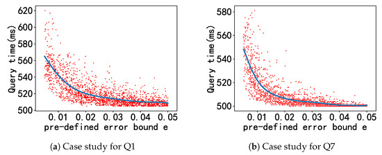
Figure 3.
Case studies: Real running time vs. predicted running time for Q1 and Q7.
5.2.2. Efficiency Evaluation
Table 6 (Efficiency results) reports the running time for our cost model, including the detail time for each step (the collect training data and training) and the total time. Note that the training data collection was the most time-consuming step, because we needed to run AQS for different predefined error bounds e to retrieve the runtime statistics. While our training was very efficient, as we did not set a high order of Taylor’s polynomial for our cost model (and we did not have a large parameter size), the normal equation performed quite efficiently. Moreover, the total time was acceptable for an offline application scenario.
Table 6.
Efficiency results for the three datasets.
5.2.3. Effect of the Size of Training Data
We varied the training data size m from 500 to 10,000, to assess its impact on the effectiveness and efficiency of our cost model. The results of the three datasets exhibited similar trends, as shown in Figure 4. (1) As m increased, the ERCM decreased and the PCM-5% increased, which was a reasonable observation, since more training data leads to an improved accuracy. (2) We observed that the accuracy improvement became stable when . (3) Both the time for training data collection and the training step increased with the increase in m, with the training data collection being more sensitive to m than the training step. (4) The time increment became more pronounced when . Ultimately, we found that by setting , we could strike a balance between the effectiveness and efficiency of our model.
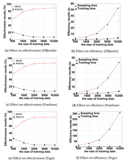
Figure 4.
Effect of the training data size on effectiveness and efficiency.
5.2.4. Discussion of the Execution Cost Model of AQS
From the results above, we can conclude that our execution cost model provided reasonably accurate predictions for AQS runtime. However, it is essential to take note of the presence of a small number of red points deviating significantly from the predicted curve in Figure 3. As clarified in Section 3.1, this “singularity” phenomenon is mainly due to the random sampling strategy employed by AQS. In rare cases, this strategy leads to the accumulation of a large number of very low-quality samples, resulting in . In this case, the AQS estimation and accuracy guarantee mechanism initiates multiple rounds of sampling, refining the CI until . This process results in a substantial increase in both and , ultimately culminating in an exceedingly prolonged query execution time. Furthermore, we observed that our execution cost model demonstrated remarkable efficiency. Nevertheless, it is essential to consider that opting for a higher order of Taylor polynomial in the cost model could enhance the accuracy but could also result in significantly increased computational costs and training time overheads. This trade-off might not be worthwhile for aggregate queries that prioritize efficiency.
5.3. Evaluation of Simple Aggregate Queries Based on the Cost Model
In this section, we used the parameters obtained from model training to find the best predefined error bound in the interval through a grid search. Within this predefined error bound, the required execution time for simple aggregate queries predicted by the model was minimal. Then, we used to run simple aggregate queries with AQS and compared its effectiveness and efficiency with comparable methods. We show the evaluation results with the default configuration as the predefined error bound and the confidence level .
5.3.1. Effectiveness and Efficiency Evaluation
It is evident from Figure 5 and Figure 6 that, first, both our model and the AQS yielded results that closely approximated the ground-truth, effectively satisfying the user-defined error criteria. Second, the response times for our model and AQS were significantly reduced in comparison to the alternative approaches. Additionally, we observed a robust correlation between our relative error and response time and those of AQS. This phenomenon can be attributed to our execution cost model, which demonstrated a tendency where the predicted execution times decreased as the predefined error bound was relaxed (as evident in Figure 3. Consequently, our value typically aligned closely with the e value used directly by AQS. However, it is worth noting that our relative error tended to be slightly larger than that of AQS, while our response time was slightly smaller. This phenomenon can be traced back to the bias introduced by the "singularity" encountered during the execution of AQS.
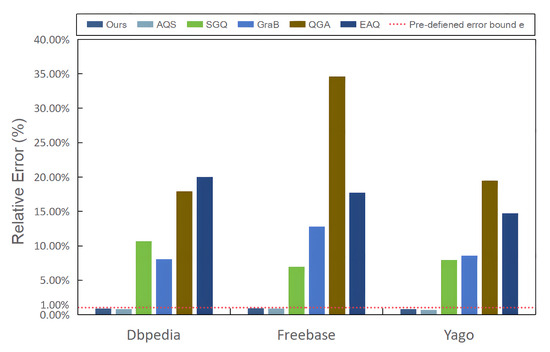
Figure 5.
Relative error of the different methods for the simple aggregate query.
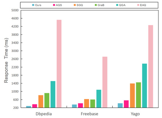
Figure 6.
Reponse time of the different methods for the simple aggregate query.
5.3.2. Discussion of Simple Aggregate Queries Based on the Cost Model
When we applied our execution cost model to simple aggregate queries, we once again confirmed the occurrence of the “singularity” phenomenon in AQS. In such instances, our model employed , which tended to be smaller than the e value use by AQS. This adjustment allowed for modest increases in the sample size during the initial round of sampling and resampling, effectively reducing the number of rounds required to satisfy the error constraints. Consequently, this prevented substantial increases in and , due to multiple rounds of sampling. However, the reduction in the number of sampling rounds resulted in an overall smaller sample size for our method when compared to AQS. As a consequence, our tended to be wider than those determined by AQS, indicating that our results may not be as precise as those provided by AQS. This observation is consistent with our research findings and underscores the need for further investigation in the domain of complex aggregate queries. At the same time, this also caused us to think that, while our approach can mitigate the impact of this “singularity” by selecting smaller error bounds and reducing the number of resampling rounds after its occurrence, it cannot fundamentally resolve the shortcomings in AQS’s sampling strategy. In future work, we may explore a better sampling strategy, such as a preference-based semantic similarity sampling strategy.
5.4. Evaluation of Complex Aggregate Queries Based on Cost Model
In this section, we first explore the imperative need for the optimization of the sub-query error bounds (Section 5.4.1). In the following section, we assess the effectiveness and efficiency of different combinations of widely employed mutation and crossover algorithms within genetic algorithms. We conducted this evaluation within the context of complex aggregate queries and identified the top-performing combination, which served as the default mutation and crossover algorithms.(Section 5.4.2). Then, we compared our method using the cost model with the optimal predefined error bounds with comparable method, in terms of effectiveness and efficiency for complex aggregate queries (Section 5.4.3). We show the experimental results with the default parameter configuration as follows: the predefined error bound for complex query , the confidence level , and the number of iterations in the genetic algorithm . Finally, we study the parameter sensitivity in Section 5.4.4.
5.4.1. Necessity of the Optimization of Sub-Queries’ Error Bounds
To illustrate the necessity of finding the optimal error bounds of all sub-queries using multi-objective optimization based on a genetic algorithm, we demonstrate the performance in terms of the relative error and response time across four different error-bound configuration strategies. These four strategies were (1) optimal error bounds (OEB), which configured sub-queries with optimal error bounds resolved by the genetic algorithm presented in Section 4. In this context, we specifically opted for the heuristic crossover and uniform mutation as the crossover and mutation techniques within the genetic algorithm. The rationale behind this choice will be elaborated upon in Section 5.4.2. (2) Minimal error bounds (MEB), which configures sub-queries with minimal error bounds, i.e., each sub-query is performed with the minimal error bound, to achieve the most accurate result. (3) Random error bounds (REB), which assigns a random error bound for a sub-query. (4) Optimal error bounds regarding sub-queries (OEB-S), which directly uses the method presented in Section 3 to compute the optimal error bound for each sub-query. From Figure 7, we can observe that both Ours-OEB and Ours-MEB could satisfy the predefined error bounds. Ours-OEB exhibited a remarkably close adherence to the predefined error bounds. Conversely, Ours-REB and Ours-OEB-S failed to meet the predefined error bound constraints. Notably, Ours-REB demonstrated the largest relative error, while Ours-OEB-S, although satisfying the error constraints for individual sub-queries, did not necessarily ensure the adherence of the complex aggregate queries to these error bounds. Furthermore, Figure 8 reveals that Ours-MEB had the highest response time, due to the stringent accuracy requirements. On the other hand, Ours-REB had the lowest response time, since the parameters were allocated randomly, essentially imposing the loosest error bound constraint. Additionally, Ours-OEB fell between Ours-OEB-S and Ours-MEB in terms of response time, as the error bound constraints of Ours-OEB were relatively looser than those of Ours-MEP, but tighter than those of Ours-OEB-S. The aforementioned observations align with our earlier conclusion that "tighter error bound constraints entail longer response times." Overall, Ours-OEB exhibited exceptional performance in terms of relative error and response time. Concurrently, the inability of Ours-OEB-S to satisfy the predefined error bound constraints underscores the necessity of the optimization of sub-query error bounds using a genetic algorithm (Section 4.2).
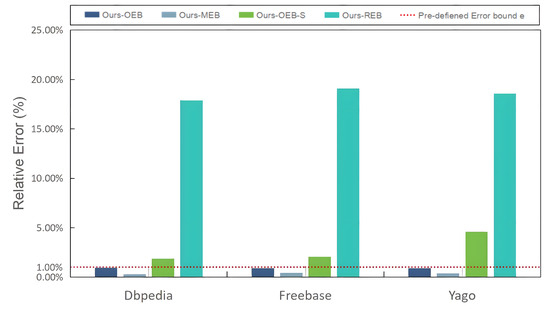
Figure 7.
Relative error under the different parameter optimization directions.
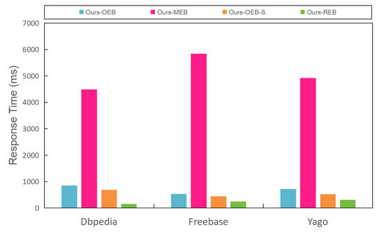
Figure 8.
Response times under different parameter optimization directions.
5.4.2. Effect of the Crossover and Mutation Algorithms Used in Genetic Algorithms
Considering the substantial influence of mutation and crossover algorithms within genetic algorithms on the eventual outcomes. To determine the combination of mutation and crossover operations with the most significant impact on parameter optimization in genetic algorithms, we chose various common crossover and mutation algorithms as combinations. We evaluated the effectiveness and efficiency of these combinations by analyzing their response time and relative error.
Since our encoding method is binary, we opted for single-point crossover(SC), heuristic crossover(HC), and uniform crossover(UC) as the crossover algorithms. For the mutation algorithms, we selected gene-wise mutation(GM), uniform mutation(UM), and inversion mutation(IM). By pairing the crossover algorithms with the mutation algorithms, we formed a total of nine combinations: (1) Ours-OEB-SC-GM; (2) Ours-OEB-SC-UM; (3) Ours-OEB-SC-IM; (4) Ours-OEB-UC-GM; (5) Ours-OEB-UC-UM; (6) Ours-OEB-UC-IM; (7) Ours-OEB-HC-GM; (8) Ours-OEB-HC-UM; (9) Ours-OEB-HC-IM.
From Figure 9, we found that “Our-OEB-SC-GM” achieved the lowest relative error. This was because the single-point crossover and basic gene-wise mutation only mildly diversified the population. However, the single-point crossover tended to become trapped in local optima, often failing to find the optimal balance point satisfying Equation (10) during sub-query parameter optimization. Tighter error bound parameters for sub-queries significantly increased the response time. Combining the data in Figure 10, we can observe that the “Our-OEB-SC-GM” method exhibited the longest overall execution time. However, it is crucial to note that the sub-query parameter optimization time for this method was relatively short. The extended execution time in this case primarily resulted from the prolonged AQS execution.
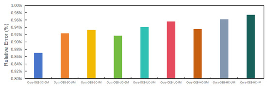
Figure 9.
Relative error under different combinations of crossover algorithms and mutation algorithms.
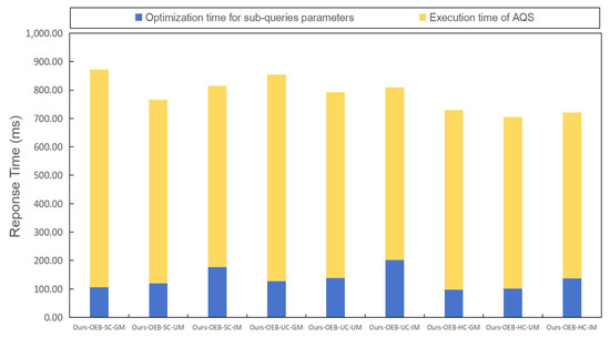
Figure 10.
Response time under different combinations of crossover algorithms and mutation algorithms.
Increasing population diversity through uniform mutation and inversion mutation comes at the cost of additional time overheads. Figure 10 illustrates that, when the crossover algorithms were the same, the gene-wise mutation combination resulted in the lowest sub-query parameter optimization time, while the inversion mutation combination led to the highest. Inversion mutation substantially increased the number of individuals to be processed and disrupted the genetic structure of good individuals, resulting in a much slower algorithm convergence. Additionally, boundary checks and validation introduced additional time overheads.
Moreover, the method with the shortest overall time was “Ours-OEB-HC-UM”. Furthermore, as shown in Figure 10, this method boasted the shortest sub-query parameter optimization time. Primarily, heuristic crossover aligned well with our problem’s characteristics. It tended to retain genes of individuals with a high fitness, making sub-queries more efficient. Simultaneously, this trait significantly reduced duplicate individual generation and accelerated genetic algorithm convergence, while uniform mutation introduced less computational overheads than inversion mutation. It effectively enhanced the population diversity without leading to local optima. Considering Figure 9, “Ours-OEB-HC-UM” was already very close to the optimal balance point between efficiency and effectiveness. Although "Our-OEB-HC-IM" was even closer, considering the time overheads introduced by inversion mutation, we lean towards using “Ours-OEB-HC-UM” as our optimal model.
5.4.3. Effectiveness and Efficiency Evaluation
Next, we assessed the effectiveness and efficiency of each method by examining the relative error and response time in the context of complex aggregate queries. Figure 11 reveals that, with the exception of Ours-OEB-HC-UM, the methods failed to meet the predefined error bounds. The explanation for AQS’s limitations was discussed in the “efficiency vs. effectiveness trade-off problem” and elsewhere, and will not be reiterated here. Regarding EAQ, GraB, and QGA, their disregard for the semantic similarity within the knowledge graph resulted in the omission of answers with similar semantics and patterns. Given that complex aggregate queries often involve multiple types of entity and predicate, these methods are prone to increased errors. As for SGQ, it adjusted its model parameters based on the query problem during querying. However, when dealing with complex aggregate queries involving multiple query problems, the model parameters were influenced by several query problems simultaneously, rendering the parameters of the model unreasonable.
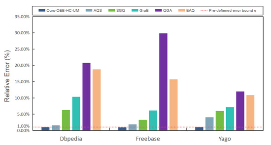
Figure 11.
The relative error of the different methods with different data.
In Figure 12, it became evident that EAQ had the longest execution time, as this required traversing all potential candidate results during querying. On the other hand, the other methods (GraB, QGA, SGQ) often employed dynamic pruning and branch strategies to adjust the search scope and avoid fruitless searches. In contrast, AQS and Ours-OEB-HC-UM employed sampling estimation to narrow down the search scope and avoid exhaustive searches. Furthermore, we observed that the execution time of AQS was slightly shorter than that of Ours-OEB-HC-UM. This was because Ours-OEB-HC-UM imposed tighter constraints on sub-queries within complex aggregate queries, to ensure adherence to the predefined error bounds. Consequently, Ours-OEB-HC-UM exhibited a longer response time. This phenomenon was also observed for simple aggregate queries.
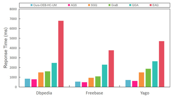
Figure 12.
The response time of the different methods with different data.
5.4.4. Parameter Sensitivity
We provide the parameter sensitivity results of Ours-OEB-HC-UM on the Dbpedia datasets, which include the predefined error bound e, genetic algorithm iteration number r, and confidence level . The results of the other datasets showed a similar trend.
- User-desired error bound e. Figure 13 presents the relative error rate and query time for the complex aggregate query results across various predefined error bounds, ranging from 1% to 5%. The results illustrated in Figure 13 effectively showcase the adaptability of the proposed method to different accuracy requirements. Additionally, a noteworthy observation gleaned from the figure revealed that as the predefined error bound became more lenient, the query response time experienced a reduction. This phenomenon closely paralleled the behavior observed in the simple aggregate queries, thus reaffirming the conclusion that "complex aggregate queries consist of multiple simple aggregate queries". The primary factor contributing to the enhanced efficiency was that a more relaxed error bound often necessitates fewer samples and sampling rounds, resulting in a reduced search space and a decrease in the number of iterations, ultimately leading to quicker query responses.
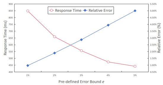 Figure 13. The response time and relative error under different predefiend error bounds.
- Iterations r. Figure 14 depicts the relative error rate and query time of the complex aggregate query results across a range of iterations for the genetic algorithm, from 10 to 1000. It is evident from Figure 11 that when the number of iterations fell within the range of 10 to 50, there was a notable increase in the relative error rate. However, once the number of iterations surpassed 50, the relative error rate remained relatively stable. This behavior stemmed from the fact that when the number of iterations was insufficient, the genetic algorithm struggled to converge towards the optimal solution that satisfied Equation (10). Consequently, the error bound remained smaller, resulting in more accurate query results.Furthermore, Figure 14 highlights that if the number of iterations was either too low or too high, this led to increased response times. There are two primary reasons for this: (1) A lower number of iterations yields inaccurate results from the genetic algorithm, causing a bias in the error bound of the sub-queries. (2) While this bias may contribute to more accurate sub-queries results, it simultaneously increases the time consumption of the sub-queries, ultimately leading to a longer complex aggregate query time. Conversely, a higher number of iterations consumes a significant amount of time during the iterative process, with marginal improvements in the relative error rate of the final result.
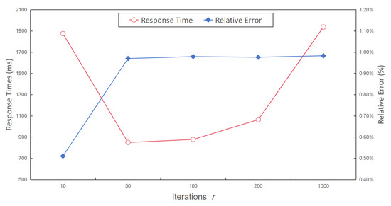 Figure 14. The response time and relative error with a different number of iterations.
- Confidence level . Figure 15 presents the relative error rate and response time for complex aggregate query results, while varying the confidence level from 86% to 98%. The results depicted in Figure 15 reveal a conspicuous trend: as the confidence level increased, the relative error rate decreased. This phenomenon can be primarily attributed to the fact that higher confidence levels correspond to smaller half-widths of the result interval, resulting in a more tightly constrained confidence interval and more precise estimated results. Furthermore, as illustrated in Figure 15, an escalation in the confidence level was associated with a gradual increase in query response time. This can be explained by the need for more query time to obtain a narrower confidence interval when striving for a higher confidence level.
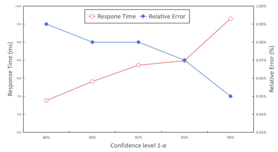 Figure 15. The response time and relative error with different confidence levels.
5.4.5. Discussion of Complex Aggregate Queries Based on the Cost Model
In the previous sections, we highlighted the importance of parameter optimization, examined various genetic algorithm crossover and mutation techniques, and evaluated our model’s performance with complex aggregate queries.
Our experiments stressed the significance of parameter optimization for precise outcomes with complex aggregate queries. The different crossover and mutation methods impacted the query efficiency differently. A single-point crossover may become trapped in local optima, while a uniform crossover slows the convergence. Tailored to our problem, the heuristic crossover emerged as the best choice, preserving solutions, reducing redundancy, and speeding up convergence. Gene-wise mutation lacks diversity expansion, and inversion mutation disrupts the genetic structures. In contrast, uniform mutation diversifies without disrupting the genetic structures. Our experimental data strongly favored heuristic crossover and uniform mutation.
Our approach excels in both effectiveness and efficiency when handling complex aggregate queries, while adhering to user-defined error bounds. The other methods, lacking optimization or relying on lower-quality factoid query results, fell short in both effectiveness and efficiency.
In our sensitivity analysis, we explored error bounds, iterations, and confidence levels. A tighter error bound ensured a higher precision but could lengthen response times. Increasing iterations introduced increased time overheads, without significant accuracy gains. Both excessively low and high confidence levels reduced the efficiency. Ultimately, we found a balance between efficiency and effectiveness, with a 95% confidence level and 50 iterations.
6. Related Work
- Online Aggregation. Online aggregation is one of the earliest approaches for performing an aggregate query. The concept of online aggregation (OLA) was initially introduced in [35]. This technology relies on sampling techniques to provide approximate aggregate outcomes within relational data contexts. Since its inception, a substantial body of subsequent research has emerged, considering various dimensions including (1) OLA implementation concerning joins and group-by operations [36,37,38,39,40,41,42], (2) OLA adaptation for distributed environments [43,44,45,46,47,48], and (3) optimizing multi-query scenarios for OLA [49,50]. However, it is important to note that none of these established approaches can be readily applied to address aggregate queries within knowledge graphs (KGs). The inherent reason behind this incompatibility is the distinctive nature of a KG’s schema-flexible structure, which significantly diverges from the rigid framework of relational data. To bridge this gap, a breakthrough was achieved in [18]. Here, a pioneering semantic-aware sampling methodology, meticulously tailored for KGs, was devised. This groundbreaking innovation acts as a pivotal solution, harmonizing traditional OLA techniques with the complex landscape of aggregate query processing within knowledge graphs.
- Factoid Query for KGs. Factoid query is an important application of knowledge graph queries, which aims to retrieve clear and factual answers from structured knowledge storage systems (such as knowledge graphs or semantic databases) in response to specific questions raised by users [4,7,12,14,51,52]. They retrieve queries for specific facts or factual information from knowledge graphs or semantic databases through keyword matching, entity recognition, and learning [4,6,7,8,9,12,13,14,15,51,52,53,54]. However, this querying method is limited to retrieving direct and factual answers from knowledge graphs or structured databases. It typically necessitates a one-to-one mapping between the query and the answer, and furthermore demands that the user provides a highly precise description of the input question. Otherwise, the query response may yield a substantial error. Simultaneously, factoid queries are unable to infer additional information concealed within the KGs. This limitation served as one of the motivations behind the introduction of aggregate queries.
- Aggregate Query for KGs. At present, the prevailing methods for addressing aggregate queries predominantly involve the utilization of fact queries, typically SPARQL aggregate queries [8,55,56,57,58] and AQS. Nevertheless, this approach frequently imposes supplementary time overheads, due to the incorporation of extra aggregate operations into the factoid query. Furthermore, the effectiveness of this approach is contingent upon the quality of the results yielded by the factoid query. However, it is worth noting that AQS still lacks the capacity to comprehensively support complex aggregate queries employing "sampling estimation" models. In light of these constraints, we introduced a pioneering cost model designed to notably enhance the efficiency and precision of complex aggregate queries.
7. Conclusions
In this paper, we first introduced an execution cost model for AQS for simple aggregate queries of KGs, using Taylor’s theorem. Then, we utilized runtime statistics gathered from AQS as training data and employed normal equations to determine the parameters of the cost model. Building upon this foundational cost mode, we developed a method explicitly tailored for addressing complex aggregate queries using AQS, which achieved a trade-off between effectiveness and efficiency. Finally, our empirical findings, based on real-world datasets, compellingly illustrated the effectiveness and efficiency of our method. In the future, we will focus on the extension of our method to aggregate queries with the MAX/MIN function and grouping by operation, thus making applicable to more general scenarios.
Author Contributions
S.Y., X.X., Y.W. and T.F. Writing—original draft. All authors were actively involved in all activities related to this paper. All authors have read and agreed to the published version of the manuscript.
Funding
This work was supported by the National NSF of China (62072149), the Primary R&D Plan of Zhejiang (2021C03156 and 2023C03198), and the Fundamental Research Funds for the Provincial Universities of Zhejiang (GK219909299001-006).
Data Availability Statement
We have shared the code and datasets we used in this research through the following GitHub link: https://github.com/KGLab-HDU/Complex-Aggregate-Queries.
Conflicts of Interest
The authors declare no conflict of interest.
References
- Guha, R.V.; McCool, R.; Miller, E. Semantic Search. In Proceedings of the WWW 2003, Budapest, Hungary, 20–24 May 2003. [Google Scholar]
- Namaki, M.H.; Song, Q.; Wu, Y.; Yang, S. Answering Why-questions by Exemplars in Attributed Graphs. In Proceedings of the SIGMOD 2019, Amsterdam, The Netherlands, 30 June 30–5 July 2019; pp. 1481–1498. [Google Scholar]
- Agichtein, E.; Cucerzan, S.; Brill, E. Analysis of Factoid Questions for Effective Relation Extraction. In Proceedings of the SIGIR 2005, Salvador, Brazil, 15–19 August 2005. [Google Scholar]
- Khan, A.; Wu, Y.; Aggarwal, C.C.; Yan, X. NeMa: Fast Graph Search with Label Similarity. PVLDB 2013, 6, 181–192. [Google Scholar]
- Zou, L.; Huang, R.; Wang, H.; Yu, J.X.; He, W.; Zhao, D. Natural Language Question Answering over RDF: A Graph Driven Approach. In Proceedings of the SIGMOD 2014, Snowbird, UT, USA, 22–27 June 2014. [Google Scholar]
- Yang, S.; Han, F.; Wu, Y.; Yan, X. Fast Top-k Search in Knowledge Graphs. In Proceedings of the ICDE 2016, Helsinki, Finland, 16–20 May 2016. [Google Scholar]
- Jin, J.; Khemmarat, S.; Gao, L.; Luo, J. Querying Web-Scale Information Networks Through Bounding Matching Scores. In Proceedings of the WWW 2015, Florence, Italy, 18–22 May 2015. [Google Scholar]
- Zou, L.; Özsu, M.T.; Chen, L.; Shen, X.; Huang, R.; Zhao, D. gStore: A Graph-based SPARQL Query Engine. VLDB J. 2014, 23, 565–590. [Google Scholar] [CrossRef]
- Wang, Y.; Khan, A.; Wu, T.; Jin, J.; Yan, H. Semantic Guided and Response Times Bounded Top-k Similarity Search over Knowledge Graphs. In Proceedings of the ICDE 2020, Dallas, TX, USA, 20–24 April 2020. [Google Scholar]
- Cui, W.; Xiao, Y.; Wang, H.; Song, Y.; Hwang, S.W.; Wang, W. KBQA: Learning Question Answering over QA Corpora and Knowledge Bases. PVLDB 2017, 10, 565–576. [Google Scholar] [CrossRef]
- Bonifati, A.; Martens, W.; Timm, T. An Analytical Study of Large SPARQL Query Logs. PVLDB 2017, 11, 149–161. [Google Scholar]
- Khan, A.; Li, N.; Yan, X.; Guan, Z.; Chakraborty, S.; Tao, S. Neighborhood Based Fast Graph Search in Large Networks. In Proceedings of the SIGMOD 2011, Athens, Greece, 12–16 June 2011. [Google Scholar]
- Yang, S.; Wu, Y.; Sun, H.; Yan, X. Schemaless and Structureless Graph Querying. PVLDB 2014, 7, 565–576. [Google Scholar] [CrossRef][Green Version]
- Fan, W.; Li, J.; Ma, S.; Wang, H.; Wu, Y. Graph Homomorphism Revisited for Graph Matching. PVLDB 2010, 3, 1161–1172. [Google Scholar] [CrossRef]
- Zheng, W.; Zou, L.; Peng, W.; Yan, X.; Song, S.; Zhao, D. Semantic SPARQL Similarity Search over RDF Knowledge Graphs. PVLDB 2016, 9, 840–851. [Google Scholar] [CrossRef]
- Lissandrini, M.; Pedersen, T.B.; Hose, K.; Mottin, D. Knowledge Graph Exploration: Where Are We and Where Are We Going? ACM SIGWEB Newsletter: New York, NY, USA, 2020. [Google Scholar]
- Wu, Y.; Khan, A. Graph Pattern Matching. In Encyclopedia of Big Data Technologies; Springer: Berlin/Heidelberg, Germany, 2019. [Google Scholar]
- Wang, Y.; Khan, A.; Xu, X.; Jin, J.; Hong, Q.; Fu, T. Aggregate Queries on Knowledge Graphs: Fast Approximation with Semantic-aware Sampling. In Proceedings of the ICDE 2022, Kuala Lumpur, Malaysia, 9–12 May 2022. [Google Scholar]
- Wang, Y.; Khan, A.; Xu, X.; Ye, S.; Pan, S.; Zhou, Y. Approximate and Interactive Processing of Aggregate Queries on Knowledge Graphs: A Demonstration. In Proceedings of the 31st ACM International Conference on Information & Knowledge Management, Atlanta, GA, USA, 17–21 October 2022; Hasan, M.A., Xiong, L., Eds.; ACM: New York, NY, USA, 2022; pp. 5034–5038. [Google Scholar] [CrossRef]
- Bao, J.; Duan, N.; Yan, Z.; Zhou, M.; Zhao, T. Constraint-based Question Answering with Knowledge Graph. In Proceedings of the COLING 2016, Osaka, Japan, 11–16 December 2016. [Google Scholar]
- Bordes, A.; Usunier, N.; Chopra, S.; Weston, J. Large-scale Simple Question Answering with Memory Networks. arXiv 2015, arXiv:1506.02075. [Google Scholar]
- Huang, X.; Zhang, J.; Li, D.; Li, P. Knowledge Graph Embedding Based Question Answering. In Proceedings of the WSDM 2019, Melbourne, Australia, 11–15 February 2019. [Google Scholar]
- Jin, J.; Khemmarat, S.; Gao, L.; Luo, J. A Distributed Approach for Top-k Star Queries on Massive Information Networks. In Proceedings of the ICPADS 2014, Hsinchu, Taiwan, 16–19 December 2014. [Google Scholar]
- Bordes, A.; Usunier, N.; García-Durán, A.; Weston, J.; Yakhnenko, O. Translating Embeddings for Modeling Multi-relational Data. In Proceedings of the NIPS 2013, Lake Tahoe, NV, USA, 5–10 December 2013. [Google Scholar]
- Li, Y.; Wu, Z.; Lin, S.; Xie, H.; Lv, M.; Xu, Y.; Lui, J.C. Walking with Perception: Efficient Random Walk Sampling via Common Neighbor Awareness. In Proceedings of the ICDE 2019, Macao, China, 8–11 April 2019. [Google Scholar]
- Mangasarian, O.L. Nonlinear Programming; SIAM: Philadelphia, PA, USA, 1994. [Google Scholar]
- Lehmann, J.; Isele, R.; Jakob, M.; Jentzsch, A.; Kontokostas, D.; Mendes, P.N.; Hellmann, S.; Morsey, M.; van Kleef, P.; Auer, S.; et al. DBpedia—A Large-Scale, Multilingual Knowledge Base Extracted from Wikipedia. Semant. Web 2015, 6, 167–195. [Google Scholar] [CrossRef]
- Bollacker, K.D.; Evans, C.; Paritosh, P.; Sturge, T.; Taylor, J. Freebase: A Collaboratively Created Graph Database for Structuring Human Knowledge. In Proceedings of the SIGMOD 2008, Vancouver, BC, Canada, 9–12 June 2008. [Google Scholar]
- Hoffart, J.; Suchanek, F.M.; Berberich, K.; Weikum, G. YAGO2: A Spatially and Temporally Enhanced Knowledge Base from Wikipedia. Artif. Intell. 2013, 194, 28–61. [Google Scholar] [CrossRef]
- QALD-4. Available online: http://qald.aksw.org/index.php?x=challenge&q=4 (accessed on 9 December 2014).
- Unger, C.; Forascu, C.; Lopez, V.; Ngomo, A.C.N.; Cabrio, E.; Cimiano, P.; Walter, S. Question Answering over Linked Data (QALD-4). In Proceedings of the Working Notes for CLEF 2014 Conference, Sheffield, UK, 15–18 September 2014. [Google Scholar]
- Berant, J.; Chou, A.; Frostig, R.; Liang, P. Semantic Parsing on Freebase from Question-answer Pairs. In Proceedings of the EMNLP 2013, Seattle, WA, USA, 18–21 October 2013. [Google Scholar]
- Han, S.; Zou, L.; Yu, J.X.; Zhao, D. Keyword Search on RDF Graphs—A Query Graph Assembly Approach. In Proceedings of the 2017 ACM on Conference on Information and Knowledge Management, CIKM 2017, Singapore, 6–10 November 2017; Lim, E., Winslett, M., Sanderson, M., Fu, A.W., Sun, J., Culpepper, J.S., Lo, E., Ho, J.C., Donato, D., Agrawal, R., et al., Eds.; ACM: New York, NY, USA, 2017; pp. 227–236. [Google Scholar] [CrossRef]
- Li, Y.; Ge, T.; Chen, C. Online Indices for Predictive Top-k Entity and Aggregate Queries on Knowledge Graphs. In Proceedings of the 2020 IEEE 36th International Conference on Data Engineering (ICDE), Dallas, TX, USA, 20–24 April 2020. [Google Scholar]
- Hellerstein, J.M.; Haas, P.J.; Wang, H.J. Online Aggregation. In Proceedings of the SIGMOD 1997, Tucson, AZ, USA, 23–15 May 1997. [Google Scholar]
- Haas, P.J.; Hellerstein, J.M. Ripple Joins for Online Aggregation. In Proceedings of the SIGMOD 1999, Philadelphia, PA, USA, 1–3 June 1999. [Google Scholar]
- Jermaine, C.M.; Arumugam, S.; Pol, A.; Dobra, A. Scalable Approximate Query Processing with the DBO Engine. In Proceedings of the SIGMOD 2007, Beijing, China, 12–14 June 2007. [Google Scholar]
- Luo, G.; Ellmann, C.J.; Haas, P.J.; Naughton, J.F. A Scalable Hash Ripple Join Algorithm. In Proceedings of the SIGMOD 2002, Madison, WI, USA, 3–6 June 2002. [Google Scholar]
- Li, F.; Wu, B.; Yi, K.; Zhao, Z. Wander Join: Online Aggregation via Random Walks. In Proceedings of the SIGMOD 2016, San Francisco, CA, USA, 26 June–1 July 2016. [Google Scholar]
- Park, Y.; Mozafari, B.; Sorenson, J.; Wang, J. VerdictDB: Universalizing Approximate Query Processing. In Proceedings of the SIGMOD 2018, Houston, TX, USA, 10–15 June 2018. [Google Scholar]
- Acharya, S.; Gibbons, P.B.; Poosala, V. Congressional Samples for Approximate Answering of Group-By Queries. In Proceedings of the SIGMOD 2000, Dallas, TX, USA, 16–18 May 2000. [Google Scholar]
- Ding, B.; Huang, S.; Chaudhuri, S.; Chakrabarti, K.; Wang, C. Sample + Seek: Approximating Aggregates with Distribution Precision Guarantee. In Proceedings of the SIGMOD 2016, San Francisco, CA, USA, 26 June–1 July 2016. [Google Scholar]
- Shi, Y.; Meng, X.; Wang, F.; Gan, Y. You Can Stop Early with COLA: Online Processing of Aggregate Queries in the Cloud. In Proceedings of the CIKM 2012, Maui, HI, USA, 29 October–2 November 2012. [Google Scholar]
- Wu, S.; Jiang, S.; Ooi, B.C.; Tan, K. Distributed Online Aggregation. PVLDB 2009, 2, 443–454. [Google Scholar] [CrossRef]
- Condie, T.; Conway, N.; Alvaro, P.; Hellerstein, J.M.; Gerth, J.; Talbot, J.; Elmeleegy, K.; Sears, R. Online Aggregation and Continuous Query Support in MapReduce. In Proceedings of the SIGMOD 2010, Indianapolis, IN, USA, 6–10 June 2010. [Google Scholar]
- Condie, T.; Conway, N.; Alvaro, P.; Hellerstein, J.M.; Elmeleegy, K.; Sears, R. MapReduce Online. In Proceedings of the NSDI 2010, San Jose, CA, USA, 28–30 April 2010. [Google Scholar]
- Pansare, N.; Borkar, V.R.; Jermaine, C.; Condie, T. Online Aggregation for Large MapReduce Jobs. PVLDB 2011, 4, 1135–1145. [Google Scholar] [CrossRef]
- Zeng, K.; Agarwal, S.; Dave, A.; Armbrust, M.; Stoica, I. G-OLA: Generalized On-Line Aggregation for Interactive Analysis on Big Data. In Proceedings of the SIGMOD 2015, Melbourne, Australia, 31 May–4 June 2015. [Google Scholar]
- Wu, S.; Ooi, B.C.; Tan, K.L. Continuous Sampling for Online Aggregation over Multiple Queries. In Proceedings of the SIGMOD 2010, Indianapolis, IN, USA, 6–10 June 2010. [Google Scholar]
- Wang, Y.; Luo, J.; Song, A.; Dong, F. OATS: Online Aggregation with Two-Level Sharing Strategy in Cloud. Distrib. Parallel Databases 2014, 32, 467–505. [Google Scholar] [CrossRef]
- Cheng, J.; Yu, J.X.; Ding, B.; Yu, P.S.; Wang, H. Fast Graph Pattern Matching. In Proceedings of the Proceedings of the 24th International Conference on Data Engineering, ICDE 2008, Cancún, México, 7–12 April 2008. [Google Scholar]
- Ma, S.; Cao, Y.; Fan, W.; Huai, J.; Wo, T. Strong simulation: Capturing topology in graph pattern matching. ACM Trans. Database Syst. (TODS) 2014, 39, 1–46. [Google Scholar] [CrossRef]
- Zheng, W.; Zou, L.; Lian, X.; Wang, D.; Zhao, D. Graph similarity search with edit distance constraint in large graph databases. In Proceedings of the 22nd ACM international Conference on Information & Knowledge Management, San Francisco, CA, USA, 27 October–1 November 2013; pp. 1595–1600. [Google Scholar]
- Zheng, W.; Lian, X.; Zou, L.; Hong, L.; Zhao, D. Online Subgraph Skyline Analysis over Knowledge Graphs. IEEE Trans. Knowl. Data Eng. 2016, 28, 1805–1819. [Google Scholar] [CrossRef]
- Hu, X.; Duan, J.; Dang, D. Scalable Aggregate Keyword Query over Knowledge Graph. Future Gener. Comput. Syst. 2020, 107, 588–600. [Google Scholar] [CrossRef]
- Unger, C.; Bühmann, L.; Lehmann, J.; Ngomo, A.N.; Gerber, D.; Cimiano, P. Template-based Question Answering over RDF Data. In Proceedings of the WWW 2012, Lyon, France, 16–20 April 2012. [Google Scholar]
- Höffner, K.; Lehmann, J.; Usbeck, R. CubeQA—Question Answering on RDF Data Cubes. In Proceedings of the ISWC 2016, Kobe, Japan, 17–21 October 2016. [Google Scholar]
- Hu, X.; Dang, D.; Yao, Y.; Ye, L. Natural Language Aggregate Query over RDF Data. Inf. Sci. 2018, 454–455, 363–381. [Google Scholar] [CrossRef]


Disclaimer/Publisher’s Note: The statements, opinions and data contained in all publications are solely those of the individual author(s) and contributor(s) and not of MDPI and/or the editor(s). MDPI and/or the editor(s) disclaim responsibility for any injury to people or property resulting from any ideas, methods, instructions or products referred to in the content. |
© 2023 by the authors. Licensee MDPI, Basel, Switzerland. This article is an open access article distributed under the terms and conditions of the Creative Commons Attribution (CC BY) license (https://creativecommons.org/licenses/by/4.0/).